To understand the performance analysis of data structures such as Treaps (chapter 3) and Bloom filters (chapter 4), we need to take a step back and first introduce a class of algorithms with which not every developer is familiar.

Most people, when prompted about algorithms, immediately think about deterministic algorithms. It’s easy to mistake this subclass of algorithms for the whole group: our common sense makes us expect an algorithm to be a sequence of instructions that, when provided a specific input, applies the same steps to return a well-defined output.

That’s indeed the common scenario. It is possible, however, to describe an algorithm as a sequence of well-defined steps that will produce a deterministic result but take an unpredictable (though finite) amount of time. Algorithms that behave this way are called Las Vegas algorithms.

Even less intuitively, it is possible to describe algorithms that might produce a different, unpredictable result for the same input in every execution, or might also not terminate in a finite amount of time. There is a name for this class of algorithms as well: they are called Monte Carlo algorithms.

There is some debate about whether the latter should be considered as algorithms or heuristics, but I lean toward including them, because the sequence of steps in Monte Carlo algorithms is deterministic and well-defined. In this book we do present a few Monte Carlo algorithms, so you will have a chance to form an educated opinion.

But before delving into these classes, we should define a particularly useful class of problems, decision problems.

F.1  Decision problems

When talking about algorithms that return either true or false, we fall into the class of problems called binary decision problems.

Binary classification algorithms assign one of two labels to the data. The two labels can actually be anything, but conceptually, this is equivalent to assigning a Boolean label to each point, so we’ll use this notation in the rest of the book.

Considering only binary classification is not restrictive, since multiclass classifiers can be obtained by combining several binary classifiers.

One fundamental result in computer science, and in particular in the field of computability and complexity, is that any optimization problem can be expressed as a decision problem and vice versa.

For instance, if we are looking for the shortest path in a graph, we can define an equivalent decision problem by setting a threshold T and checking if there exists a path with length at most T. By solving this problem for different values of T, and by choosing these values using binary search, we can find a solution to the optimization problem by using an algorithm for the decision problem.¹

F.2  Las Vegas algorithms

The class of so-called Las Vegas algorithms includes all randomized algorithms that

1. Always give as output the correct solution to the problem (or return a failure).

2. Can be run using a finite, but unpredictable (random) amount of resources. The key point is that how much resources are needed can’t be predicted based on input.

The most notable example of a Las Vegas algorithm is probably randomized quicksort:² it always produces the correct solution, but the pivot is chosen randomly at every recursive step, and execution time swirls between O(n*log n) and O(n2), depending on the choices made.

F.3  Monte Carlo algorithms

We classify algorithms as Monte Carlo methods when the output of the algorithm can sometimes be incorrect. The probability of an incorrect answer is usually a trade-off with the resources employed, and practical algorithms manage to keep this probability small while using a reasonable amount of computing power and memory.

For decision problems, when the answer to a Monte Carlo algorithm is just true/false, we have three possible situations:

• The algorithm is always correct when it returns false (so-called false-biased algorithm).

• The algorithm is always correct when it returns true (so-called true-biased algorithm).

• The algorithm might return the wrong answer indifferently for the two cases.

Monte Carlo algorithms are deterministic in the amount of resources needed, and they are used often as the dual of a Las Vegas algorithm.

Suppose we have an algorithm A that always return the correct solution, but whose resource consumption is not deterministic. If we have a limited amount of resources, we can run A until it outputs a solution or exhausts the allotted resources. For instance, we could stop randomized quicksort after n*log n swaps.

This way, we are trading accuracy (the guarantee of a correct result) for the certainty to have a (sub-optimal) answer within a certain time (or using at most a certain amount of space).

It’s also worth noting that as we mentioned, for some randomized algorithms, we don’t even know if they will eventually stop and find a solution (although this is usually not the case). Take, for example, the randomized version of Bogosort.

F.4  Classification metrics

When we analyze data structures such as Bloom filters or Treaps, examining the time and memory requirements of their methods is paramount, but not enough. Besides how fast they run, and how much memory they use, for Monte Carlo algorithms like these we also need to ask one more question: “How well does it work?”

To answer this question, we need to introduce metrics, functions that measure the distance between an approximated solution and the optimal one.

For classification algorithms, the quality of an algorithm is a measure of how well each input is assigned to its right class. For binary (that is, true/false) classification, therefore, it’s about how accurately the algorithm outputs true for the input points.

F.4.1  Accuracy

One way of measuring the quality of a classification algorithm is to assess the rate of correct predictions. Suppose that over N_P points actually belonging to the true class:

• PP are predicted as true.

• TP, the so-called true positives, are both predicted as true and actually belong to the true class.

Likewise, let NN be the number of points belonging to the false class:

• PN is the total number of points for which our algorithm predicts the class false.

• TN, the so-called true negatives, is the number of times both the predicted and the actual class of a point are false.

Then we can define accuracy:

When the accuracy is 1, we have an algorithm that is always correct.

Unfortunately, except for that ideal case, accuracy is not always a good measure of the quality of our algorithms. Consider an edge case where 99% of the points in a database actually belongs to the true class. Then look at the following three classifiers:

• A classifier correctly labeling 100% of the false points and 98.98% of the true ones

• A classifier correctly labeling 0.5% of the false points and 99.49% of the true ones

• A classifier that always returns true as label

Astonishingly, the latter has better accuracy than the other two, even if it misses every single point in the false category.

Tip If you’d like to double check this, plug in these numbers into the formula for accuracy.

In machine learning, if you were to use this metric on a training set skewed in a similar way,³ you’d get a terrible model, or more precisely, a model that is likely to generalize poorly.

F.4.2  Precision and recall

To improve over bare accuracy, we need to keep track of the info about each category separately. To this end, we can define two new metrics:

• Precision (also called positive predictive value) defined as the ratio of correctly predicted true points (the true positives) over the total number of points for which true was predicted by the algorithm:

  

• Recall (also known as sensitivity) defined as the fraction of true positives over the total number of actual positives:

  

It is possible to give an alternate definition of precision and recall by introducing the number of false positives Fp, that is, points belonging to the false class for which true was incorrectly predicted, and the number of false negatives Fn:

Intuitively, while accuracy only measures how well we do on predictions, precision/recall metrics weigh our successes with our errors for the dual category. As a matter of fact, precision and recall are not independent, and one can be defined in terms of the other, so it’s not possible to improve both indefinitely. In general, if you improve recall, you’ll often get a slightly worse precision and vice versa.

For machine learning classifiers, every model can be associated with a precision/recall curve (see figure F.1), and the model’s parameters can be tuned during training so that we can trade off the two characteristics.

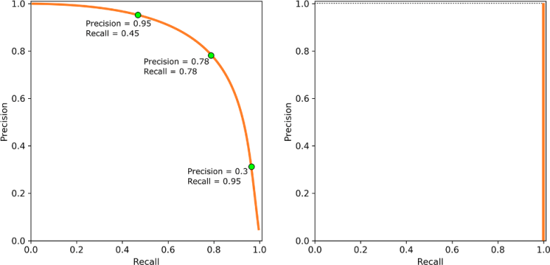
Figure F.1 Examples of precision-recall curve. The one on the left is a generic curve for a hypothetical algorithm. This is plotted by tuning the algorithm’s parameters and recording the precision and recall obtained. After recording many attempts, we can get a drawing similar to this graphic. In general, when a given choice of the model’s parameters improves precision, there will be a slight worsening of recall, and vice versa. On the right, a degenerate P-R curve for a false-biased algorithm, such as Bloom filters; its recall is always equal to 1, for any precision. True-biased algorithms have a symmetrical P-R curve.

So, for binary categorization, a perfect (100%) precision means that every point for which we output true actually belonged to the true category. Similarly, for recall, when it’s 100%, we never have a false negative.

As an exercise, try to compute precision and recall for the examples in the previous sections and see how they give us more information about the quality of a model with respect to just its accuracy.

If we take Bloom filters (chapter 4) as an example, we explain in section 4.8 that when the output is false, we can be sure it’s right, so Bloom filters have a 100% recall.

Their precision, unfortunately, is not as perfect. In section 4.10 we delve into the details of how to compute it. In this case, however, like for all false-biased algorithms, there is no trade-off with recall, and improving precision can only be done by increasing the resources used.

F.4.3  Other metrics and recap

There are, of course, other metrics that can be useful for classifiers. One of the most useful is the F-measure,⁴ combining precision and recall into one formula. These alternative metrics, however, go beyond our scope.

If we continue with our parallel with Bloom filters, we can recap the meaning of the metrics we examined in that context:

• Accuracy answers the question, “What percentage of calls to contains are correct?”

• Precision answers the question, “What percentage of calls to contains returning true were correct?”

• Recall answers the question, “Among all calls to contains on elements actually contained in the filter, what percent of them returned true?” (This one, as we know, will always be 100% for Bloom filters).

---

^1. If the threshold is guaranteed to be an integer or rational number, we can also guarantee that the solution will be in the same computational class as the solution to the decision problem, so if, for example, we have a polynomial solution to the decision problem, solving the optimization problem will also require polynomial time.

^2. See Grokking Algorithms, by Aditya Bhargava (Manning Publications, 2016), chapter 4, page 51.

^3. For instance, a dataset where one of the classes is rare or difficult to get data for: this is often the case in medicine with rare diseases.

^4. See https://en.wikipedia.org/wiki/F1_score.