This chapter covers

• Discussing the limits of k-d trees
• Describing image retrieval as a use case where k-d trees would struggle
• Introducing a new data structure, the R-tree
• Presenting SS-trees, a scalable variant of R-trees
• Comparing SS-trees and k-d trees
• Introducing approximate similarity search

This chapter will be structured slightly differently from our book’s standard, because we will continue here a discussion started in chapter 8. There, we introduced the problem of searching multidimensional data for the nearest neighbor(s) of a generic point (possibly not in the dataset itself). In chapter 9, we introduce k-d trees, a data structure specifically invented to solve this problem.

K-d trees are the best solution to date for indexing low- to medium-dimensional datasets that will completely fit in memory. When we have to operate on high-dimensional data or with big datasets that won’t fit in memory, k-d trees are not enough, and we will need to use more advanced data structures.

In this chapter we first present a new problem, one that will push our indexing data structure beyond its limits, and then introduce two new data structures, R-trees and SS-trees, that can help us solve this category of problems efficiently.

Brace yourself—this is going to be a long journey (and a long chapter!) through some of the most advanced material we have presented so far. We’ll try to make it through this journey step by step, section by section, so don’t let the length of this chapter intimidate you!

10.1 Right where we left off

Let’s briefly recap where we left off in previous chapters. We were designing software for an e-commerce company, an application to find the closest warehouse selling a given product for any point on a very large map. Check out figure 9.4 to visualize it. To have a ballpark idea of the kind of scale we need, we want to serve millions of clients per day across the country, taking products from thousands of warehouses also spread across the map.

In section 8.2, we have already established that a brute-force approach is not practical for applications at scale, and we need to resort to a brand-new data structure designed to handle multidimensional indexing. Chapter 9 described k-d trees, a milestone in multidimensional data indexing and a true game changer, which worked perfectly with the example we used in chapters 8 and 9 where we only needed to work with 2-D data. The only issue we faced is the fact that our dataset was dynamic and thus insertion/removal would produce an imbalanced tree, but we could rebuild the tree every so often (for instance, after 1% of its elements had been changed because of insertions or removals), and amortize the cost of the operation by running it in a background process (keeping the old version of the tree in the meantime, and either putting insert/delete on hold, or reapplying these operations to the new tree once it had been created and “promoted” to current).

While in that case we could find workarounds, in other applications we won’t necessarily be so lucky. There are, in fact, intrinsic limitations that k-d trees can’t overcome:

• K-d trees are not self-balancing, so they perform best when they are constructed from a stable set of points, and when the number of inserts and removes is limited with respect to the total number of elements.

• The curse of dimensionality: When we deal with high-dimensional spaces, k-d trees become inefficient, because running time for search is exponential in the dimension of the dataset. For points in the k-dimensional space, when k ≈ 30, k-d trees can’t give any advantage over brute-force search.

• K-d trees don’t work well with paged memory, because they are not memory-efficient with respect to the locality of reference, as points are stored in tree nodes, so nearby points won’t lie close to memory areas.

10.1.1 A new (more complex) example

To illustrate a practical situation where k-d trees are not the recommended solution, let’s pivot on our warehouse search and imagine a different scenario, where we fast-forward 10 years. Our e-commerce company has evolved and doesn’t sell just groceries anymore, but also electronics and clothes. It’s almost 2010, and customers expect valuable recommendations when they browse our catalog; but even more importantly, the company’s marketing department expects that you, as CTO, make sure to increase sales by showing customers suggestions they actually like.

For instance, if customers are browsing smartphones (the hottest product in the catalog, ramping up to rule the world of electronics, back in the day!), your application is supposed to show them more smartphones in a similar price/feature range. If they are looking at a cocktail dress, they should see more dresses that look similar to the one they (possibly) like.

Now, these two problems look (and partially are) quite different, but they both boil down to the same core issue: given a product with a list of features, find one or more products with similar features. Obviously, the way we extract these feature lists from a consumer electronics product and a dress is very different!

Let’s focus on the latter, illustrated in figure 10.1. Given an image of a dress, find other products in your catalog that look similar—this is a very stimulating problem, even today!

Figure 10.1 Feature extraction on an image dataset. Each image is translated into a feature vector (through what’s represented as a “black box” feature extractor, because we are not interested in the algorithm that creates this vectors). Then, if we have to search an entry P, we compare P’s feature vector to each of the images’ vectors, computing their mutual distance based on some metric. (In the figure, Euclidean distance. Notice that when looking for the minimum of these Euclidean distances, we can sometimes compute the squared distances, avoiding applying a square root operation for each entry.)

The way we extract features from images completely changed in the last 10 years. In 2009, we used to extract edges, corners, and other geometrical features from the images, using dozens of algorithms specialized for the single feature, and then build higher-level features by hand (quite literally).

Today, instead, we use deep learning for the task, training a CNN¹ on a larger dataset and then applying it to all the images in our catalog to generate their feature vectors.

Once we have these feature vectors, though, the same question arises now as then: How do we efficiently search the most similar vectors to a given one?

This is exactly the same problem we illustrated in chapter 8 for 2-D data, applied to a huge dataset (with tens of thousands of images/feature vectors), and where tuples have hundreds of features.

Contrary to the feature extraction, the search algorithms haven’t changed much in the last 10 years, and the data structures that we introduce in this chapter, invented between the late 1990s and the early 2000s, are still cutting-edge choices for efficient search in the vector space.

10.1.2 Overcoming k-d trees’ flaws

Back in chapter 9, we also mentioned a couple of possible structural solutions to cope with the problems discussed in the previous section:

• Instead of partitioning points using a splitting line passing through a dataset’s points, we can divide a region into two balanced halves with respect to the number of points or the sub-region’s size.

• Instead of cycling through dimensions, we can choose at every step the dimension with the greatest spread or variance and store the choice made in each tree node.

• Instead of storing points in nodes, each node could describe a region of space and link (directly or indirectly) to an array containing the actual elements.

These solutions are the basis of the data structures we will discuss in this chapter, R-trees and SS-trees.

10.2 R-tree

The first evolution of k-d trees we will discuss are R-trees. Although we won’t delve into the details of their implementation, we are going to discuss the idea behind this solution, why they work, and their high-level mechanism.

R-trees were introduced in 1984 by Antonin Guttman in the paper “R-Trees. A Dynamic Index Structure For Spatial Searching.”

They are inspired by B-trees,² balanced trees with a hierarchical structure. In particular, Guttman used as a starting point B+ trees, a variant where only leaf nodes contain data, while inner nodes only contain keys and serve the purpose of hierarchically partitioning data.

10.2.1 A step back: Introducing B-trees

Figure 10.2 shows an example of a B-tree, in particular a B+tree. These data structures were meant to index unidimensional data, partitioning it into pages,³ providing efficient storage on disk and fast search (minimizing the number of pages loaded, and so the number of disk accesses).

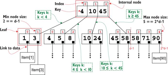
Figure 10.2 B+ tree explained. The example shows a B+ tree with a branching factor of d == 3.

Each node (both internal nodes and leaves) in a B-tree contains between d-1 and 2*d-1 keys, where d is a fixed parameter for each tree, its branching factor:⁴ the (minimum, in this case) number of children for each node. The only exception can be the root, which can possibly contain fewer than d-1 keys. Keys are stored in an ordered list; this is fundamental to have a fast (logarithmic) search. In fact, each internal node with m keys, k0, k1, ..., km-1, d-1 ≤ m ≤ 2*d*-1, also has exactly m+1 children, C0, C1, ..., Cm-1, Cm, such that k < k0 for each key k in the subtree rooted in C0; k0 ≤ k < k1 for each key k in the subtree rooted in C1; and so on.

In a B-tree, keys and items are stored in the nodes, each key/item is stored exactly once in a single node, and the whole tree stores exactly n keys if the dataset has n items. In a B+ tree, internal nodes only contains keys, and only leaves contain pairs, each with keys and links to the items. This means that a B+tree storing n items has n leaves, and that keys in internal nodes are also stored in all its descendants (see how, in the example in figure 10.2, the keys 4, 10, and 45 are also stored in leaves).

Storing links to items in the leaves, instead of having the actual items hosted in the tree, serves a double purpose:

• Nodes are more lightweight and easier to allocate/garbage collect.

• It allows storing all items in an array, or in a contiguous block of memory, exploiting the memory locality of neighboring items.

When these trees are used to store huge collections of large items, these properties allow us to use memory paging efficiently. By having lightweight nodes, it is more likely the whole tree will fit in memory, while items can be stored on disk, and leaves can be loaded on a need-to basis. Because it is also likely that after accessing an item X, applications will need to access one of its contiguous items, by loading in memory the whole B-tree leaf containing X, we can reduce the disk reads as much as possible.

Not surprisingly, for these reasons B-trees have been the core of many SQL database engines since their invention⁵—and even today they are still the data structure of choice for storing indices.

10.2.2 From B-Tree to R-tree

R-trees extend the main ideas behind B+trees to the multidimensional case. While for unidimensional data each node corresponds to an interval (the range from the left-most and right-most keys in its sub-tree, which are in turn its minimum and maximum keys), in R-trees each node N covers a rectangle (or a hyper-rectangle in the most generic case), whose corners are defined by the minimum and maximum of each coordinate over all the points in the subtree rooted at N.

Similarly to B-trees, R-trees are also parametric. Instead of a branching factor d controlling the minimum number of entries per node, R-trees require their clients to provide two parameters on creation:

• M, the maximum number of entries in a node; this value is usually set so that a full node will fit in a page of memory.

• m, such that m ≤ M/2, the minimum number of entries in a node. This parameter indirectly controls the minimum height of the tree, as we’ll see.

Given values for these two parameters, R-trees abide by a few invariants:

1. Every leaf contains between m and M points (except for the root, which can possibly have less than m points).

2. Each leaf node L has associated a hyper-rectangle RL, such that RL is the smallest rectangle containing all the points in the leaf.

3. Every internal node has between m and M children (except for the root, which can possibly have less than m children).

4. Each internal node N has associated a bounding (hyper-)rectangle RN, such that RN is the smallest rectangle, whose edges are parallel to the Cartesian axes, entirely containing all the bounding rectangles of N’s children.

5. The root node has at least two children, unless it is a leaf.

6. All leaves are at the same level.

Property number 6 tells us that R-trees are balanced, while from properties 1 and 3 we can infer that the maximum height of an R-tree containing n points is logM(n).

On insertion, if any node on the path from the root to the leaf holding the new point becomes larger than M entries, we will have to split it, creating two nodes, each with half the elements.

On removal, if any node becomes smaller than m entries, we will have to merge it with one of its adjacent siblings.

Invariants 2 and 4 require some extra work to be maintained true, but these bounding rectangles defined for each node are needed to allow fast search on the tree.

Before describing how the search methods work, let’s take a closer look at an example of an R-tree in figures 10.3 and 10.4. We will stick to the 2-D case because it is easier to visualize, but as always, you have to imagine that real trees can hold 3-D, 4-D, or even 100-D points.

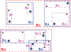
Figure 10.3 Cartesian plane representation of a (possible) R-tree for our city maps as presented in the example of figure 9.4 (the names of the cities are omitted to avoid confusion). This R-tree contains 12 bounding rectangles, from R1 to R12, organized in a hierarchical structure. Notice that rectangles can and do overlap, as shown in the bottom half.

If we compare figure 10.3 to figure 9.6, showing how a k-d tree organizes the same dataset, it is immediately apparent how the two partitionings are completely different:

• R-trees create regions in the Cartesian plane in the shape of rectangles, while k-d trees split the plane along lines.

• While k-d trees alternate the dimension along which the split is done, R-trees don’t cycle through dimensions. Rather, at each level the sub-rectangles created can partition their bounding box in any or even all dimensions at the same time.

• The bounding rectangles can overlap, both across different sub-trees and even with siblings’ bounding boxes sharing the same parent. However, and this is crucial, no sub-rectangle extends outside its parent’s bounding box.

• Each internal node defines a so-called bounding envelope, that for R-trees is the smallest rectangle containing all the bounding envelopes of the node’s children.

Figure 10.4 shows how these properties translate into a tree data structure; here the difference with k-d trees is even more evident!

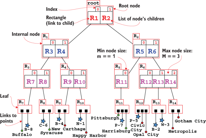
Figure 10.4 The tree representation for the R-tree from figure 10.3. The parameters for this R-tree are m==1 and M==3. Internal nodes only hold bounding boxes, while leaves hold the actual points (or, in general, k-dimensional entries). In the rest of the chapter we will use a more compact representation, for each node drawing just the list of its children.

Each internal node is a list of rectangles (between m and M of them, as mentioned), while leaves are lists of (again, between m and M) points. Each rectangle is effectively determined by its children and could indeed be defined iteratively in terms of its children. For practical reasons such as improving the running time of the search methods, in practice we store the bounding box for each rectangle.

Because the rectangles can only be parallel to the Cartesian axes, they are defined by two of their vertices: two tuples with k coordinates, one tuple for the minimum values of each coordinate, and one for the maximum value of each coordinate.

Figure 10.5 R-trees entries, besides points, can also be rectangles or non-zero-measure entities. In this example, entities R7 to R14 are the tree’s entries, while R3 to R6 are the tree’s leaves.

Notice how unlike k-d trees, an R-tree could handle a non-zero-measure object by simply considering its bounding boxes as special cases of rectangles, as illustrated in figure 10.5.

10.2.3 Inserting points in an R-tree

Now, of course, you might legitimately wonder how you get from a raw dataset to the R-tree in figure 10.5. After all, we just presented it and asked you to take it as a given.

Insertion for R-trees is similar to B-trees and has many steps in common with SS-trees, so we won’t duplicate the learning effort with a detailed description here.

At a high level, to insert a new point you will need to follow the following steps:

1. Find the leaf that should host the new point P. There are three possible cases:

   1. P lies exactly within one of the leaves’ rectangles, R. Then just add P to R and move to the next step.

   2. P lies within the overlapping region between two or more leaves’ bounding rectangles. For example, referring to figure 10.6, it might lie in the intersection of R12 and R14. In this case, we need to decide where to add P; the heuristic used to make these decisions will determine the shape of the tree (as an example, one heuristic could be just adding it to the rectangle with fewer elements).

   3. If P lies outside of all rectangles at the leaves’ level, then we need to find the closest leaf L and add P to it (again, we can use more complex heuristics than just the Euclidean distance to decide).

2. Add the points to the leaf’s rectangle R, and check how many points it contains afterward:

   1. If, after the new point is added, the leaf still has at most M points, then we are done.

   2. Otherwise, we need to split R into two new rectangles, R1 and R2, and go to step 3.

3. Remove R from its parent RP and add R1 and R2 to RP. If RP now has more than M children, split it and repeat this step recursively.

   1. If R was the root, we obviously can’t remove it from its parent; we just create a new root and set R1 and R2 as children.

To complete the insertion algorithm outlined here, we need to provide a few heuristics to break ties for overlapping rectangles and to choose the closest rectangle, but even more importantly, we haven’t said anything about how we are going to split a rectangle at points 2 and 3.

Figure 10.6 Choosing the R-tree leaf’s rectangle to which a point should be added: the new point can lie within a leaf rectangle (PA), within the intersection of two or more leaves’ rectangles (PB), or outside any of the leaves (PC and PD).

This choice, together with the heuristic for choosing the insertion subtree, determines the behavior and shape (not to mention performance) of the R-tree.

Several heuristics have been studied over the years, each one aiming to optimize one or more usages of the tree. The split heuristics can be particularly complicated for internal nodes because we don’t just partition points, but k-dimensional shapes. Figure 10.7 shows how easily a naïve choice could lead to inefficient splits.

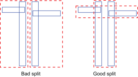
Figure 10.7 An example of bad and good splits of an internal node’s rectangle, taken from the original paper by Antonin Guttman

Delving into these heuristics is out of the scope of this section; we refer the curious reader to the original paper by Antonin Guttman for a proper description. At this point, though, we can already reveal that the complexity of handling hyper-rectangles and obtaining good splits (and merges, after removals) is one of the main reasons that led to the introduction of SS-trees.

10.2.4 Search

Searching for a point or for the nearest neighbor (NN ) of a point in R-trees is very similar to what happens in k-d trees. We need to traverse the tree, pruning branches that can’t contain a point, or, for NN search, are certainly further away than the current minimum distance.

Figure 10.8 shows an example of an (unsuccessful) point search on our example R-tree. Remember that an unsuccessful search is the first step for inserting a new point, through which we can find the rectangle (or rectangles, in this case) where we should add the new point.

Figure 10.8 Unsuccessful search on the R-tree in figures 10.4 and 10.5. The path of the search is highlighted in both the Cartesian and tree views, and curved arrows show the branches traversed in the tree. Notice the compact representation of the tree, compared to figure 10.5.

The search starts at the root, where we compare point P’s coordinates with the boundaries of each rectangle, R1 and R2; P can only be within R2, so this is the only branch we traverse.

At the next step, we go through R2’s children, R5 and R6. Both can contain P, so we need to traverse both branches at this level (as shown by the two curved arrows, leaving R2 in the bottom half of figure 10.8).

This means we need to go through the children of both rectangles R5 and R6, checking from R11 to R14. Of these, only R12 and R14 can contain P, so those are the only rectangles whose points we will check at the last step. Neither contains P, so the search method can return false, and optionally the two leaves’ rectangles that could host P, if inserted.

Nearest neighbor search works similarly, but instead of checking whether a point belongs to each rectangle, it keeps the distance of the current nearest neighbor and checks to see if each rectangle is closer than that (otherwise, it can prune it). This is similar to the rectangular region search in k-d trees, as described in section 9.3.6.

We won’t delve into NN-search for R-trees. Now that you should have a high-level understanding of this data structure, we are ready to move on to its evolution, the SS-tree.

It’s also worth mentioning that R-trees do not guarantee good worst-case performance, but in practice they usually perform better than k-d trees, so they were for a long time the de facto standard for similarity search and indexing of multidimensional datasets.

10.3 Similarity search tree

In section 10.2, we saw some of the key properties that influence the shape and performance of R-trees. Let’s recap them here:

• The splitting heuristic

• The criteria used to choose the sub-tree to add new points (if more than one overlaps)

• The distance metric

For R-trees, we assumed that aligned boxes, hyper-rectangles parallel to the Cartesian axes, are used as bounding envelopes for the nodes. If we lift this constraint, the shape of the bounding envelope becomes the fourth property of a more general class of similarity search trees.

And, indeed, at their core, the main difference between R-trees and SS-trees in their most basic versions, is the shape of bounding envelopes. As shown in figure 10.9, this variant (built on R-trees) uses spheres instead of rectangles.

Figure 10.9 Representation of a possible SS-tree covering the same dataset of figures 10.4 and 10.5, with parameters m==1 and M==3. As you can see, the tree structure is similar to R-trees’. For the sake of avoiding clutter, only a few spheres’ centroids and radii are shown. For the tree, we use the compact representation (as shown in figures 10.5 and 10.8).

Although it might seem like a small change, there is strong theoric and practical evidence that suggest using spheres reduces the average number of leaves touched by a similarity (nearest neighbor or region) query. We will discuss this point in more depth in section 10.5.1.

Each internal node N is therefore a sphere with a center and a radius. Those two properties are uniquely and completely determined by N’s children. N’s center is, in fact, the centroid of N’s children,⁶ and the radius is the maximum distance between the centroid and N’s points.

To be fair, when we said that the only difference between R-trees and SS-trees was the shape of the bounding envelopes, we were guilty of omission. The choice of a different shape for the bounding envelopes also forces us to adopt a different splitting heuristic. In the case of SS-trees, instead of trying to reduce the spheres’ overlap on split, we aim to reduce the variance of each of the newly created nodes; therefore, the original splitting heuristic chooses the dimension with the highest variance and then splits the sorted list of children to reduce variance along that dimension (we’ll see this in more detail in the discussion about insertion in section 10.3.2).

As for R-trees, SS-trees have two parameters, m and M, respectively the minimum and maximum number of children each node (except the root) is allowed to have.

And like R-trees, bounding envelopes in an SS-tree might overlap. To reduce the overlap, some variants like SS₊-trees introduce a fifth property (also used in R-tree’s variants like R*-trees), another heuristic used on insert that performs major changes to restructure the tree; we will talk about SS+-trees later in this chapter, but for now we will focus on the implementation of plain SS-trees.

The first step toward a pseudo-implementation for our data structures is, as always, presenting a pseudo-class that models it. In this case, to model an SS-tree we are going to need a class modeling tree nodes. Once we build an SS-tree through its nodes, to access it we just need a pointer to the tree’s root. For convenience, as shown in listing 10.1, we will include this link and the values for parameters m and M in the SsTree class, as well as the dimensionality k of each data entry, and assume all these values are available from each of the tree nodes.

As we have seen, SS-trees (like R-trees) have two different kind of nodes, leaves and internal nodes, that are structurally and behaviorally different. The former stores k-dimensional tuples (references to the points in our dataset), and the latter only has links to its children (which are also nodes of the tree).

To keep things simple and as language-agnostic as possible, we will store both an array of children and an array of points into each node, and a Boolean flag will tell apart leaves from internal nodes. The children array will be empty for leaves and the points array will be empty for internal nodes.

Listing 10.1 The SsTree and SsNode classes

class SsNode
  #type tuple(k)
  centroid
  #type float
  radius
 
  #type SsNode[]
  children
 
  #type tuple(k)[]
  points
  
  #type boolean
  Leaf
 
  function SsNode(leaf, points=[], children=[])
 
class SsTree
  #type SsNode
  root
  #type integer 
  m
  #type integer 
  M
  #type integer 
  k
 
  function SsTree(k, m, M)

Notice how in figure 10.9 we represented our tree nodes as a list of spheres, each of which has a link to a child. We could, of course, add a type SsSphere and keep a link to each sphere’s only child node as a field of this new type. It wouldn’t make a great design, though, and would lead to data duplication (because then both SsNode and SsSphere would hold fields for centroids and radius) and create an unnecessary level of indirection. Just keep in mind that when you look at the diagrams of SS-trees in these pages, what are shown as components of a tree node are actually its children.

One effective alternative to translate this into code in object-oriented programming is to use inheritance, defining a common abstract class (a class that can’t be instantiated to an actual object) or an interface, and two derived classes (one for leaves and one for internal nodes) that share a common data and behavior (defined in the base, abstract class), but are implemented differently. Listing 10.2 shows a possible pseudo-code description of this pattern.

Listing 10.2 Alternative Implementation for SsNode: SsNodeOO

abstract class SsNodeOO
  #type tuple(k)
  centroid
  #type float
  radius
   
class SsInnerNode: SsNodeOO
  #type SsNode[]
  children
  function SsInnerNode(children=[])
 
class SsLeaf: SsNodeOO
  #type tuple(k)[]
  points
  function SsLeaf(points=[])

Although the implementation using inheritance might result in some code duplication and greater effort being required to understand the code, it arguably provides a cleaner solution, removing the logic to choose the type of node that would otherwise be needed in each method of the class.

Although we won’t adopt this example in the rest of the chapter, the zealous reader might use it as a starting point to experiment with implementing SS-trees using this pattern.

10.3.1 SS-tree search

Now we are ready to start describing SsNode’s methods. Although it would feel natural to start with insertion (we need to build a tree before searching it, after all), it is also true that as for many tree-based data structures, the first step to insert (or delete) an entry is searching the node where it should be inserted.

Hence, we will need the search method (meant as exact element search) before we can insert a new item. While we will see how this step in the insert method is slightly different from plain search, it will still be easier to describe insertion after we have discussed traversing the tree.

Figures 10.10 and 10.11 show the steps of a call to search on our example SS-tree. To be fair, the SS-tree we’ll use in the rest of the chapter is derived from the one in figure 10.9. You might notice that there are a few more points (the orange stars), a few of the old points have been slightly moved, and we stripped all the points’ labels, replacing them with letters from A to W, in order to remove clutter and have cleaner diagrams. For the same reason, we’ll identify the point to search/insert/delete, in this and the following sections, as Z (to avoid clashes with points already in the tree).

Figure 10.10 Search on a SS-tree: the first few steps of searching for point Z. The SS-tree shown is derived from the one in figure 10.9, with a few minor changes; the name of the entries have been removed here and letters from A to W are used to reduce clutter. (Top) The first step of the search is comparing Z to the spheres in the tree’s root: for each of them, computes the distance between Z and its centroid, and checks if it’s smaller than the sphere’s radius. (Bottom) Since both S1 and S2 intersect Z, we need to traverse both branches and check spheres S3 to S6 for intersection with Z.

To continue with our image dataset example, suppose that we now would like to check to see if a specific image Z is in our dataset. One option would be comparing Z to all images in the dataset. Comparing two images might require some time (especially if, for instance, all images have the same size, and we can’t do a quick check on any other trivial image property to rule out obviously different pairs). Recalling that our dataset supposedly has tens of thousands of images, if we go this way, we should be prepared to take a long coffee break (or, depending on our hardware, leave our machine working for the night).

But, of course, by now readers must have learned that we shouldn’t despair, because this is the time we provide a better alternative!

And indeed, as we mentioned at the beginning of the chapter, we can create a collection of feature vectors for the images in our dataset, extract the feature vector for Z—let’s call it FZ—and perform a search in the feature vectors space instead of directly searching the image dataset.

Now, comparing FZ to tens or hundreds of thousands of other vectors could also be slow and expensive in terms of time, memory, and disk accesses.

If each memory page stored on disk can hold M feature vectors, we would have to perform n/M disk accesses and read n*k float values from disk.

And that’s exactly where an SS-tree comes into play. By using an SS-tree with at most M entries per node, and at least m≤M/2, we can reduce the number of pages loaded from disk to⁷ 2*logM(n), and the number of float values read to ~k*M*logM(n).

Listing 10.3 shows the pseudo-code for SS-tree’s search method. We can follow the steps from figures 10.10 and 10.11. Initially node will be the root of our example tree, so not a leaf; we’ll then go directly to line #7 and start cycling through node’s children, in this case S1 and S2.

Listing 10.3 The search method

function search(node, target)                        ❶
  if node.leaf then                                  ❷
    for point in node.points do                      ❸
      if point == target then
        return node                                  ❹
  else
    for childNode in node.children do                ❺
      if childNode.intersectsPoint(target) then      ❻
        result ← search(childNode, target)           ❼
        if result != null then                       ❼
          return result                              ❼
  return null                                        ❽

❶ Method search returns the tree leaf that contains a target point if the point is stored in the tree; it returns null otherwise. We explicitly pass the root of the (sub)tree we want to search so we can reuse this function for sub-trees.

❷ Checks if node is a leaf or an internal node

❸ If node is a leaf, goes through all the points held, and checks whether any match target

❹ If a match is found, returns current leaf

❺ Otherwise, if we are traversing an internal node, goes through all its children and checks which ones could contain target. In other words, for each children childNode, we check the distance between its centroid and the target point, and if this is smaller than the bounding envelope’s radius of childNode, we recursively traverse childNode.

❻ Checks if childNode could contain target; that is, if target is within childNode’s bounding envelope. See listing 10.4 for an implementation.

❼ If that’s the case, performs a recursive search on childNode’s branch, and if the result is an actual node (and not null), we have found what we were looking for and we can return.

❽ If no child of current node could contain the target, or if we are at a leaf and no point matches target, then we end up at this line and just return null as the result of an unsuccessful search.

For each of them, we compute the distance between target (point Z in the figure) and the spheres’ centroids, as shown in listing 10.4, describing the pseudo-code implementation of method SsNode::intersectsPoint. Since for both the spheres the computed (Euclidean) distance is smaller than their radii, this means that either (or both) could contain our target point, and therefore we need to traverse both S1 and S2 branches.

This is also apparent in figure 10.10, where point Z clearly lies in the intersection of spheres S1 and S2.

Figure 10.11 Search on an SS-tree: Continuing from figure 10.10, we traverse the tree up to leaves. At each step, the spheres highlighted are the ones whose children are being currently traversed (in other words, at each step the union of the highlighted spheres is the smallest area where the searched point could lie).

The next couple of steps in figures 10.10 (bottom half) and 10.11 execute the same lines of code, cycling through node’s children until we get to a leaf. It’s worth noting that this implementation will perform a depth-first traversal of the node: it will sequentially follow down to leaves, getting to leaves as fast as possible, back-tracking when needed. For the sake of space, these figures show these paths as they were traversed in parallel, which is totally possible with some modifications to the code (that would, however, be dependent on the programming language of an actual implementation, so we will stick with the simpler and less resource-intensive sequential version).

The method will sometime traverse branches where none of the children might contain the target. That’s the case, for instance, with the node containing S3 and S4. The execution will just end up at line #12 of listing 10.3, returning nulland back-tracking to the caller. It had initially traversed branch S1; now the for-each loop at line #7 will just move on to branch S2.

When we finally get to leaves S12-S14, the execution will run the cycle at line #3, where we scan a leaf’s points searching for an exact match. If we find one, we can return the current leaf as the result of the search (we assume the tree doesn’t contain duplicates, of course).

Listing 10.4 shows a simple implementation for the method checking whether a point is within a node’s bounding envelope. As you can see, the implementation is very simple, because it just uses some basic geometry. Notice, however, that the distance function is a structural parameter of the SS-tree; it can be the Euclidean distance in a k-dimensional space, but it can also be a different metric.⁸

Listing 10.4 Method SsNode::intersectsPoint

function SsNode:: intersectsPoint(point)                 ❶
  return distance(this.centroid, point) <= this.radius   ❷

❶ Method intersectsPoint is defined on SsNode. It takes a point and returns true if the point is within the bounding envelope of the node.

❷ Since the bounding envelope is a hyper-sphere, it just needs to check that the distance between the node’s centroid and the argument point is within the node’s radius. Here, distance can be any valid metric function, including (by default) the Euclidean distance in Rk.

10.3.2 Insert

As mentioned, insertion starts with a search step. While for more basic trees, such as binary search trees, an unsuccessful search returns the one and only node where the new item can be added, for SS-trees we have the same issue we briefly discussed in section 10.2 for R-trees: since nodes can and do overlap, there could be more than one leaf where the new point could be added.

This is such a big deal that we mentioned it as the second property determining the SS-tree’s shape. We need to choose a heuristic method to select which branch to traverse, or to select one of the leaves that would already contain the new point.

SS-trees originally used a simple heuristic: at each step, they would select the one branch whose centroid is closest to the point that is being inserted (those rare ties that will be faced can be broken arbitrarily).

This is not always ideal, because it might lead to a situation like the one shown in figure 10.12, where a new point Z could be added to a leaf already covering it, and instead ends up in another leaf whose envelope becomes larger to accept Z, and ends up overlapping the other leaf. It is also possible, although unlikely, that the leaf selected is not actually the closest one to the target. Since at each level we traverse only the closest node, if the tree is not well balanced, it might happen that at some point during traversal the method bumps into a skewed sphere, with the center of mass far away from a small leaf—something like S6 in figure 10.12, whose child S14 lies far away from its center of mass.

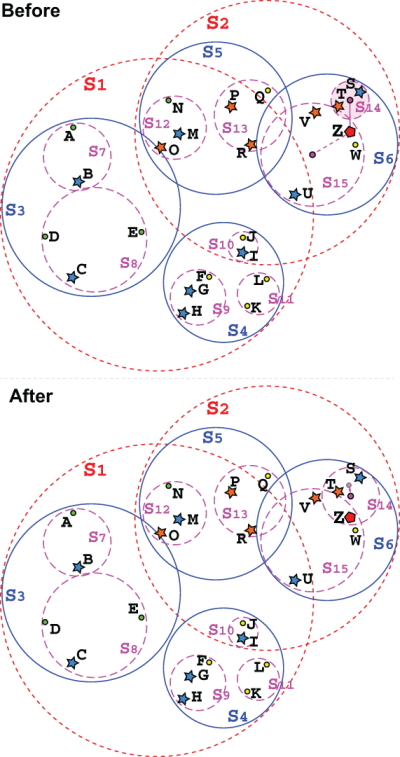
Figure 10.12 An example where the point Z, which will be inserted into the tree, is added to the closest leaf, S14, whose bounding envelope becomes larger as a result, and overlaps another existing leaf, S15, which could have held Z within its bounding envelope. In the bottom half, notice how S14’s centroid moves as a result of adding the new point to the sphere.

On the other hand, using this heuristic greatly simplifies the code and improves the running time. This way, we have a worst-case bound (for this operation) of O(logM(n)), because we only follow one path from the root to a leaf. If we were to traverse all branches intersecting Z, in the worst case we could be forced to visit all leaves.

Moreover, the code would also become more complicated because we might have to handle differently the cases where no leaf, exactly one leaf, or more than one leaf intersecting Z are found.

So, we will use here the original heuristic described in the SS-tree first paper, shown in listing 10.5. It can be considered a simpler version of the search method described in section 10.3.1, since it will only traverse a single path in the tree. Figure 10.13 shows the difference with a call to the search method for the same tree and point (refer to figures 10.10 and 10.11 for a comparison).

Listing 10.5 The searchParentLeaf method

function searchParentLeaf(node, target)      ❶
  if node.leaf then                          ❷
    return node                                
  else
    child ← node.findClosestChild(target)    ❸
    return searchParentLeaf(child, target)   ❹

❶ This search method returns the closest tree leaf to a target point.

❷ Checks if node is a leaf. If it is, we can return it.

❸ Otherwise, we are traversing an internal node and need to find which branch to go next. We run the heuristic findClosestChild to decide (see listing 10.8 for an implementation).

❹ Recursively traverses the chosen branch and returns the result

However, listing 10.5 is just meant to illustrate how this traversal works. In the actual insert method, we won’t call it as a separate step, but rather integrate it. That’s because finding the closest leaf is just the first step; we are far from being done with insertion yet, and we might need to backtrack our steps. That’s why we are implementing insert as a recursive function, and each time a sub-call returns, we backtrack on the path from the root to current node.

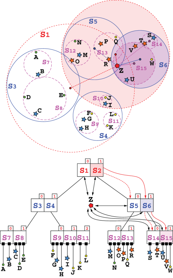
Figure 10.13 An example of the tree traversing for method searchParentLeaf. In contrast with figures 10.10 and 10.11, here the steps are condensed into a single diagram for the sake of space. The fact that only one path is traversed allows this compact representation. Notice how at each step the distance between Z and the centroids in the current node are computed (in this figure, we used for distances the same level-based color code as for spheres, and the segments drawn for distances have one end in the center of the sphere they are computed from, so it’s easy to spot the distance to the root node, and to spheres at level 1, and so on), and only the branch with the shortest distance (drawn as a thicker, solid line) is chosen. The spheres’ branches traversed are highlighted on both representations.

Suppose, in fact, that we have found that we should add Z to some leaf L, that already contains j points. We know that j ≥ m > 1, so the leaf is not empty, but there could be three very different situations:

1. If L already contains Z, we don’t do anything, assuming we don’t support duplicates (otherwise, we can refer to the remaining two cases).

2. j < M—In this case, we add Z to the list of L’s children, recompute the centroid and radius for L, and we are done. This case is shown in figure 10.12, where L==S14. On the left side of the figure, you can see how the centroid and radius of the bounding envelopes are updated as a result of adding Z to S14.

3. j == M—This is the most complicated case, because if we add another point to L, it will violate the invariant requiring that a leaf holds no more than M points. The only way to solve this is by splitting the leaf’s point into two sets and creating two new leaves that will be added to L’s parent, N. Unfortunately, by doing this we can end up in the same situation as if N already had M children. Again, the only way we can cope with this is by splitting N’s children into two sets (defining two spheres), removing N from its parent P, and adding the two new spheres to P. Obviously, P could also now have M+1 children! Long story short, we need to backtrack to the root, and we can only stop if we get to a node that has less than M children, or if we do get to the root. If we have to split the root, then we will create a new root with just two children, and the height of the tree will grow by 1 (and that’s the only case where this can happen).

Listing 10.6 shows an implementation of the insert method using the cases just described:

• The tree traversal, equivalent to the searchParentLeaf method, appears at lines #10 and #11.

• Case 1 is handled at line #3, where we return null to let the caller know there is no further action required.

• Case 2 corresponds to lines #6 and #18 in the pseudo-code, also resulting in the method returning null.

• Case 3, which clearly is the most complicated option, is coded in lines #19 and #20.

• Backtracking is handled at lines #12 to #21.

Figures 10.14 and 10.15 illustrate the third case, where we insert a point in a leaf that already contains M points. At a high level, insertion in SS-trees follows B-tree’s algorithm for insert. The only difference is in the way we split nodes (in B-trees the list of elements is just split into two halves). Of course, in B-trees links to children and ordering are also handled differently, as we saw in section 10.2.

Figure 10.14 Inserting a point in a full leaf. (Top) The search step to find the right leaf. (Center) A closeup of the area involved. S9 needs to be updated, recomputing its centroid and radius. T hen we can find the direction along which points have the highest variance (y, in the example) and split the points so that the variance of the two new point sets is minimal. Finally, we remove S9 from its parent S4 and add two new leaves containing the two point sets resulting from the split. (Bottom) The final result is that we now need to update S4’s centroid and radius and backtrack.

Figure 10.15 Backtracking in method insert after splitting a leaf. Continuing from figure 10.14, after we split leaf S9 into nodes S16 and S17, we backtrack to S9’s parent S4, and add these two new leaves to it, as shown at the end of figure 10.14. S4 now has four children, one too many. We need to split it as well. Here we show the result of splitting S4 into two new nodes, S18 and S19, that will be added to S4’s parent, S1, to which, in turn, we will backtrack. Since it now has only three children (and M==3) we just recompute centroid and radius for S1’s bounding envelope, and we can stop backtracking.

In listing 10.6 we used several helper functions⁹ to perform insertion; however, there is still one case that is not handled. What happens when we get to the root and we need to split it?

The reason for not handling this case as part of the method in listing 10.6 is that we would need to update the root of the tree, and this is an operation that needs to be performed on the tree’s class, where we do have access to the root.

Listing 10.6 The insert method

function insert(node, point)                                ❶
  if this.leaf then                                         ❷
    if point in this.points then                            ❸
      return null
    this.points.add(point)                                  ❹
    this.updateBoundingEnvelope()                           ❺
    if this.points.size <= M then                           ❻
      return null
  else
    closestChild ← this.findClosestChild()                  ❼
    (newChild1, newChild2) ← insert(closestChild, point)    ❽
    if newChild1 == null then                               ❾
      node.updateBoundingEnvelope()
      return null
    else
      this.children.delete(closestChild)                    ❿
      this.children.add(newChild1)                          ⓫
      this.children.add(newChild2)                          ⓫
      node.updateBoundingEnvelope()                         ⓬
      if this.children.size <= M then                       ⓭
        return null
  return this.split()                                       ⓮

❶ Method insert takes a node and a point and adds the point to the node’s subtree. It is defined recursively and returns null if node doesn’t need to be split as a result of the insertion; otherwise, it returns the pair of nodes resulting from splitting node.

❷ Checks if node is a leaf

❸ If it is a leaf, checks if it already contains the argument among its points, and if it does, we can return

❹ Otherwise, adds the point to the leaf

❺ We need to recompute the centroid and radius for this leaf after adding the new point.

❻ If we added a new point, we need to check whether this leaf now holds more than M points. If there are no more than M, we can return; otherwise, we continue to line #22.

❼ If we are in an internal node, we need to find which branch to traverse, calling a helper method.

❽ Recursively traverses the tree and inserts the new point, storing the outcome of the operation

❾ If the recursive call returned null, we only need to update this node’s bounding envelope, and then we can in turn return null as well.

❿ Otherwise, it means that closestchild has been split, and we need to remove it from the list of children . . .

⓫ . . . and add the two newly generated spheres in its place.

⓬ We need to compute the centroid and radius for this node.

⓭ If the number of children is still within the max allowed, we are done with backtracking.

⓮ If it gets here, it means that the node needs to be split: create two new nodes and return them.

Therefore, we will give an explicit implementation of the tree’s method for insert. Remember, we will actually only expose methods defined on the data structure classes (KdTree, SsTree, and so on) and not on the nodes’ classes (such as SsNode), but we usually omit the former’s when they are just wrappers around the nodes’ methods. Look at listing 10.7 to check out how we can handle root splits. Also, let me highlight this again: this code snippet is the only point where our tree’s height grows.

Listing 10.7 The SsTree::insert method

function SsTree::insert(point)                                      ❶
  (newChild1, newChild2) ← insert(this.root, point)                 ❷
  if newChild1 != null then                                         ❸
    this.root = new SsNode(false, children=[newChild1, newChild2])  ❸

❶ Method insert is defined on SsTree. It takes a point and doesn’t return anything.

❷ Calls the insert function on the root and stores the result

❸ If, and only if, the result of insert is not null, it needs to replace the old tree root with a newly created node, which will have as its children the two nodes resulting from splitting the old root.

10.3.3 Insertion: Variance, means, and projections

Now let’s get into the details of the (many) helper methods we call in listing 10.6, starting with the heuristic method, described in listing 10.8, to find a node’s closest child to a point Z. As mentioned, we will just cycle through a node’s children, compute the distance between their centroids and Z, and choose the bounding envelope that minimizes it.

Listing 10.8 The SsNode::findClosestChild method

function SsNode::findClosestChild(target)                        ❶
  throw-if this.leaf                                             ❷
  minDistance ← inf                                              ❸
  result ← null                                                  ❸
  for childNode in this.children do                              ❹
    if distance(childNode.centroid, point) < minDistance then    ❺
      minDistance ← distance(childNode.centroid, point)          ❻
      result ← childNode                                         ❻
  return result                                                  ❼

❶ Method findClosestChild is defined on SsNode. It takes a point target and returns the child of the current node whose distance to target is minimal.

❷ If we call this method on a leaf, there is something wrong. In some languages, we can use assert to make sure the invariant (not node.leaf) is true.

❸ Properly initializes the minimum distance, and the node that will be returned. Another implicit invariant is that an internal node has at least one child (there must be at least m), so these values will be updated at least once.

❹ Cycles through all children

❺ Checks if the distance between the current child’s centroid and target is smaller than the minimum found so far

❻ If it is, stores the new minimum distance and updates the closest node

❼ After the for loop cycles through all children, returns the closest one found

Figure 10.16 shows what happens when we need to split a leaf. First we recompute the radius and centroid of the leaf after including the new point, and then we also compute the variance of the M+1 points’ coordinates along the k directions of the axis in order to find the direction with the highest variance; this is particularly useful with skewed sets of points, like S9 in the example, and helps to reduce spheres volume and, in turn, overlap.

Figure 10.16 Splitting a leaf along a non-optimal direction. In this case, the x axis is the direction with minimal variance. Comparing the final result to figure 10.14, although S4’s shape doesn’t change significantly, S16 has more than doubled in size and completely overlaps S17; this means that any search targeted within S17 will also have to traverse S16.

If you refer to figure 10.16, you can see how a split along the x axis would have produced two sets with points G and H on one side, and F and Z on the other. Comparing the result with figure 10.14, there is no doubt about which is the best final result!

Of course, the outcome is not always so neat. If the direction of maximum variance is rotated at some angle with respect to the x axis (imagine, for instance, the same points rotated 45° clockwise WRT the leaf’s centroid), then neither axis direction will produce the optimal result. On average, however, this simpler solution does help.

So, how do we perform the split? We start with listing 10.9, which describes the method to find the direction with maximum variance. It’s a simple method performing a global maximum search in a linear space.

Listing 10.9 The SsNode::directionOfMaxVariance method

function SsNode::directionOfMaxVariance()                       ❶
  maxVariance ← 0                                               ❷
  directionIndex ← 0                                            ❷
  centroids ← this.getEntriesCentroids()                        ❸
  for i in {0..k-1} do                                          ❹
    if varianceAlongDirection(centroids, i) > maxVariance then  ❺
      maxVariance ← varianceAlongDirection(centroids, i)        ❻
      directionIndex ← i                                        ❻
  return directionIndex                                         ❼

❶ Method directionOfMaxVariance is defined on SsNode. It returns the index of the direction along which the children of a node have maximum variance.

❷ Properly initializes the maximum variance and the index of the direction with max variance

❸ Gets the centroids of the items inside the node’s bounding envelope. For a leaf, those are the points held by the leaf, while for an internal node, the centroids of the node’s children.

❹ Cycles through all directions: their indices, in a k-dimensional space, go from 0 to k-1.

❺ Checks whether the variance along the i-th axis is larger than the maximum found so far

❻ If it is, stores the new maximum variance and updates the direction’s index

❼ After the for loop cycles through all axis’ directions, returns the index of the direction for which we have found the largest variance

We need, of course, to compute the variance at each step of the for loop at line #5. Perhaps this is the right time to remind you what variance is and how it is computed. Given a set S of real values, we define its mean μ as the ratio between the sum of the values and their multiplicities:

Once we’ve defined the mean, we can then define the variance (usually denoted as σ²) as the mean of the squares of the differences between S’s mean and each of its elements:

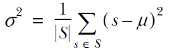
So, given a set of n points P0..Pn-1, each Pj with coordinates (P(j,0), P(j,1), .., P(j,k-1)), the formulas for mean and variance along the direction of the i-th axis are

These formulas are easily translatable into code, and in most programming languages you will find an implementation of the method computing variance in core libraries; therefore, we won’t show the pseudo-code here. Instead, let’s see how both functions for variance and mean are used in the updateBoundingEnvelope method (listing 10.10) that computes a node centroid and radius.

Listing 10.10 The SsNode:: updateBoundingEnvelope method

function SsNode::updateBoundingEnvelope()                                 ❶
  points ← this.getCentroids()                                            ❷
  for i in {0..k-1} do                                                    ❸
    this.centroid[i] ← mean{point[i] for point in points}                 ❹
  this.radius ← 
    max{distance(this.centroid, entry)+entry.radius for entry in points}  ❺

❶ Method updateBoundingEnvelope is defined on SsNode. It updates the centroid and radius for the current node.

❷ Gets the centroids of the items inside the node’s bounding envelope. For a leaf, those are the points held by the leaf, while for an internal node, the centroids of the node’s children.

❸ Cycles through the k coordinates of the (k-dimensional) space

❹ For each coordinate, computes the centroid’s value as mean of the points’ values for that coordinate. For instance, for the x axis, computes the mean of all x coordinates over all points/children in the node.

❺ The radius is the maximum distance between the node’s centroid and its children’s envelope. This distance includes the (Euclidean) distance between the two centroids, plus the radius of the children. We assume that points here have radius equal to 0.

This method computes the centroid for a node as the center of mass of its children’s centroids. Remember, for leaves, their children are just the points it contains, while for internal nodes, their children are other nodes.

The center of mass is a k-dimensional point, each of whose coordinates is the mean of the coordinates of all the other children’s centroids.¹⁰

Once we have the new centroid, we need to update the radius of the node’s bounding envelope. This is defined as the minimum radius for which the bounding envelope includes all the bounding envelopes for the current node’s children; in turn, we can define it as the maximum distance between the current node’s centroid and any point in its children. Figure 10.17 shows how and why these distances are computed for each child: it’s the sum of the distance between the two centroids and the child’s radius (as long as we assume that points have radius==0, this definition also works for leaves).

Figure 10.17 Computing the radius of an internal node. The point in SC that is further away from SA’s centroid A is the point on the bounding envelope that’s furthest from C along the opposite direction WRT SA’s centroid, and its distance is therefore the sum of the distance A-C between the two centroids, plus SC’s radius. If we choose another point P on the bounding envelope, its distance from A must be smaller than the distance A-B, because metrics by definition need to obey the triangular inequality, and the other two edges of triangle ACP are AC and CP, which is SC’s radius. You can check that this is also true for any of the other envelopes in the figure.

10.3.4 Insertion: Split nodes

We can now move to the implementation of the split method in listing 10.11.

Listing 10.11 The SsNode::split method

function SsNode::split()                                               ❶
  splitIndex ← this.findSplitIndex(coordinateIndex)                    ❷
  if this.leaf then
    newNode1 ← new SsNode(true, points=this.points[0..splitIndex-1])   ❸
    newNode2 ← new SsNode(true, points=this.points[splitIndex..])      ❸
  else
    newNode1 ← new SsNode(false, children=this.children[0.. index-1])  ❹
    newNode2 ← new SsNode(false, children=this.children [index..])     ❹
  return (newNode1, newNode2)                                          ❺

❶ Method split is defined on SsNode. It returns the two new nodes resulting from the split.

❷ Finds the best “split index” for the list of points (leaves) or children (internal nodes)

❸ If this is a leaf, the new nodes resulting from the split will be two leaves, each with part of the points of the current leaf. Given splitIndex, the first leaf will have all points from the beginning of the list to splitIndex (not included), and the other leaf will have the rest of the points list.

❹ If this node is internal, then we create two new internal nodes, each with one of the partitions of the children list.

❺ Returns the pair of new SsNodes created

This method looks relatively simple, because most of the leg work is performed by the auxiliary method findSplitIndex, described in listing 10.12.

Listing 10.12 The SsNode::findSplitIndex method

function SsNode::findSplitIndex()                                     ❶
  coordinateIndex ← this.directionOfMaxVariance()                     ❷
  this.sortEntriesByCoordinate(coordinateIndex)                       ❸
  points ← {point[coordinateIndex] for point in this.getCentroids()}  ❹
  return minVarianceSplit(points, coordinateIndex)                    ❺

❶ Method findSplitIndex is defined on SsNode. It returns the optimal index for a node split. For a leaf, the index refers to the list of points, while for an internal node it refers to the children’s list. Either list will be sorted as a side effect of this method.

❷ Finds along which axes the coordinates of the entries’ centroids have the highest variance

❸ We need to sort the node’s entries (either points or children) by the chosen coordinate.

❹ Gets a list of the centroids of this node’s entries: a list of points for a leaf, and a list of the children’s centroids, in case we are at an internal node. Then, for each centroid, extract only the coordinate given by coordinateIndex.

❺ Finds and returns which index will result in a partitioning with the minimum total variance

After finding the direction with maximum variance, we sort¹¹ points or children (depending on if a node is a leaf or an internal node) based on their coordinates for that same direction, and then, after getting the list of centroids for the node’s entries, we split this list, again along the direction of max variance. We’ll see how to do that in a moment.

Before that, we again ran into the method returning the centroids of the entries within the node’s bounding envelope, so it’s probably the right time to define it! As we mentioned before, the logic of the method is dichotomic:

• If the node is a leaf, this means that it returns the points contained in it.

• Otherwise it will return the centroids of the node’s children.

Listing 10.13 puts this definition into pseudo-code.

Listing 10.13 The SsNode::getEntriesCentroids method

function SsNode::getEntriesCentroids()                  ❶
  if this.leaf then                                     ❷
    return this.points                                  ❷
  else
    return {child.centroid for child in this.children}  ❸

❶ Method getEntriesCentroids is defined on SsNode. It returns the centroids of the entries within the node’s bounding envelope.

❷ If the node is a leaf, we can just return its points.

❸ Otherwise, we need to return a list of all the centroids of this node’s children. We use a construct typically called list-comprehension to denote this list (see appendix A).

After retrieving the index of the split point, we can actually split the node entries. Now we need two different conditional branches to handle leaves and internal nodes differently: we need to provide to the node constructors the right arguments, depending on the type of node we want to create. Once we have the new nodes constructed, all we need to do is return them.

Hang tight; we aren’t done yet. I know we have been going through this section for a while now, but we’re still missing one piece of the puzzle to finish our implementation of the insert method: the splitPoints helper function.

This method might seem trivial, but it’s actually a bit tricky to get it right. Let’s say it needs at least some thought.

So, let’s first go through an example, and then write some pseudo-code for it! Figure 10.18 illustrates the steps we need to perform such a split. We start with a node containing eight points. We don’t know, and don’t need to know, if those are dataset points or nodes’ centroids; it is irrelevant for this method.

Figure 10.18 Splitting a set of points along the direction of maximum variance. (Top) The bounding envelope and its points to split; the direction of maximum variance is along the y axis (center), so we project all points on this axis. On the right, we rotate the axis for convenience and replace the point labels with indices. (Middle) Given that there are 8 points, we can infer M must be equal to 7. Then m can be any value ≤3. Since the algorithm chooses a single split index, partitioning the points on its two sides, and each partition needs to have at least m points, depending on the actual value of m, we can have a different number of choices for the split index. (Bottom) We show the three possible resulting splits for the case where m==3: the split index can be 3, 4, or 5. We will choose the option for which the sum of the variances for the two sets is minimal.

Suppose we have computed the direction of maximum variance and that it is along the y axis; we then need to project the points along this axis, which is equivalent to only considering the y coordinate of the points because of the definition of our coordinate system.

In the diagram we show the projection of the points, since it’s visually more intuitive. For the same reason, we then rotate the axis and the projections 90° clockwise, remove the points’ labels, and index the projected points from left to right. In our code, we would have to sort our points according to the y coordinate (as we saw in listing 10.12), and then we can just consider their indices; an alternative could be using indirect sorting and keeping a table of sorted/unsorted indices, but this would substantially complicate the remaining code.

As shown, we have eight points to split. We can deduce that the parameter M, the maximum number of leaves/children for a tree node, is equal to 7, and thus m, the minimum number of entries, can only be equal to 2 or 3 (technically it could also be 1, but that’s a choice that would produce skewed trees, and usually it’s not even worth implementing these trees if we use m==1).

It’s worth mentioning again that the value for m must be chosen at the time of creation of our SS-Tree, and therefore it is fixed when we call split. Here we are just reasoning about how this choice influences how the splits are performed, and ultimately the structure of the tree.

And indeed, this value is crucial to the split method, because each of the two partitions created will need to have at least m points; therefore, since we are using a single index split,¹² the possible values for this split index go from m to M-m. In our example, as shown in the middle section of figure 10.18, this means

• If m==2, then we can choose any index between 2 and 6 (5 choices).

• If m==3, then the alternatives are between 3 and 5 (3 choices).

Now suppose we had chosen m==3. The bottom section of figure 10.18 shows the resulting split for each of the three alternative choices we have for the split index. We will have to choose the one that minimizes variance for both nodes (usually, we minimize the sum of the variances), but we only minimize variance along the direction we perform the split, so in the example we will only compute the variance of the y coordinates of the two sets of points. Unlike with R-trees, we won’t try to minimize the bounding envelopes’ overlap at this stage, although it turns out that reducing variance along the direction that had the highest variance brings us, as an indirect consequence, a reduction of the average overlap of the new nodes.

Also, with SS+-trees, we will tackle the issue of overlapping bounding envelopes separately.

For now, to finish with the insertion method, please look at listing 10.14 for an implementation of the minVarianceSplit method. As mentioned, it’s just a linear search among M – 2*(m-1) possible options for the split index of the points.

Listing 10.14 The minVarianceSplit method

function minVarianceSplit(values)                 ❶
  minVariance ← inf                               ❷
  splitIndex ← m                                  ❷
  for i in {m, |values|-m} do                     ❸
    variance1 ← variance(values[0..i-1])          ❹
    variance2 ← variance(values[i..|values|-1])   ❹
    if variance1 + variance2 < minVariance then   ❺
      minVariance ← variance1 + variance2         ❺
      splitIndex ← i                              ❺
  return splitIndex                               ❻

❶ Method minVarianceSplit takes a list of real values. The method returns the optimal index for a node split of the values. In particular, it returns the index of the first element of the second partition; the split is optimal with respect to the variance of the two sets. The method assumes the input is already sorted.

❷ Initializes temporary variables for the minimum variance and the index where to split the list

❸ Goes through all the possible values for the split index. One constraint is that both sets need to have at least m points, so we can exclude all choices for which the first set has less than m elements, as well as those where the second set is too small.

❹ For each possible value i for the split index, selects the points before and after the split, and computes the variances of the two sets

❺ If the sum of the variances just computed is better than the best result so far, updates the temporary variables

❻ Returns the best option found

And with this, we can finally close this section about SsTree::insert. You might feel this was a very long road to get here, and you’d be right: this is probably the most complicated code we’ve described so far. Take your time to read the last few sub-sections multiple times, if it helps, and then brace yourself: we are going to delve into the delete method next, which is likely even more complicated.

10.3.5 Delete

Like insert, delete in SS-trees is also heavily based on B-tree’s delete. The former is normally considered so complicated that many textbooks skip it altogether (for the sake of space), and implementing it is usually avoided as long as possible. The SS-tree version, of course, is even more complicated than the original one.

But one of the aspects where R-trees and SS-trees overcome k-d trees is that while the latter is guaranteed to be balanced only if initialized on a static dataset, both can remain balanced even when supporting dynamic datasets, with a large volume of insertions and removals. Giving up on delete would therefore mean turning down one of the main reasons we need this data structure.

The first (and easiest) step is finding the point we would like to delete, or better said, finding the leaf that holds that point. While for insert we would only traverse one path to the closest leaf, for delete we are back at the search algorithm described in section 10.3.1; however, as for insert, we will need to perform some backtracking, and hence rather than calling search, we will have to implement the same traversal in this new method.¹³

Once we have found the right leaf L, assuming we do find the point Z in the tree (otherwise, we wouldn’t need to perform any change), we have a few possible situations—an easy one, a complicated one, and a seriously complicated one:

1. If the leaf contains more than m points, we just delete Z from L, and update its bounding envelope.

2. Otherwise, after deleting Z, L will have only m-1 points, and therefore it would violate one of the SS-tree’s invariants. We have a few options to cope with this:

   1. If L is the root, we are good, and we don’t have to do anything.

   2. If L has at least one sibling S with more than m points, we can move one point from S to L. Although we will be careful to choose the closest point to L (among all its siblings with at least m+1 points), this operation can potentially cause L’s bounding envelope to expand significantly (if only siblings far away from L have enough points) and unbalance the tree.

   3. If no sibling of L can “lend” it a point, then we will have to merge L with one of its siblings. Again, we would then have to choose which sibling to merge it with and we might choose different strategies:

      1. Choosing the closest sibling

      2. Choosing the sibling with larger overlap with L

      3. Choosing the sibling that minimizes the coordinates variance (over all axes)

Case 2(c) is clearly the hardest to handle. Case 2(b), however, is relatively easy because, luckily, one difference with B-trees is that the node’s children don’t have to be sorted, so we don’t need to perform rotations when we move one point from S to L. In the middle-bottom sections of figure 10.19 you can see the result of node S3 “borrowing” one of the S4 children, S9—it’s just as easy as that. Of course, the hardest part is deciding which sibling to borrow from and which of its children should be moved.

For case 2(b), merging two nodes will cause their parent to have one less child; we thus have to backtrack and verify that this node still has at least m children. This is shown in the top and middle sections of figure 10.19. The good news is that we can handle internal nodes exactly as we handle leaves, so we can reuse the same logic (and mostly the same code) for leaves and internal nodes.

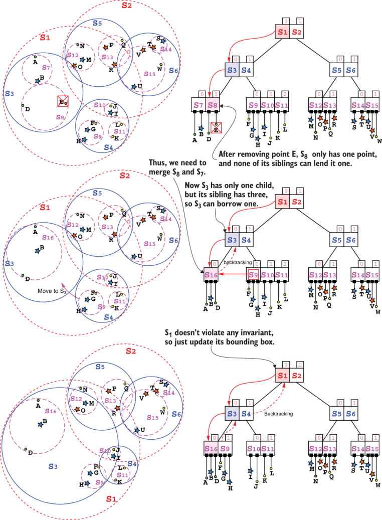
Figure 10.19 Deleting a point. This example shows, in order, cases 2(c), 2(b), and 1 described in this section.

Cases 1 (at the bottom of figure 10.19) and 2(a) are trivial, and we can easily implement them; the fact that when we get to the root we don’t have to do any extra action (like we have to for insert) makes the SsTree::delete wrapper method trivial.

Enough with the examples; it’s time to write the body of the delete method, shown in listing 10.15.

Listing 10.15 The delete method

function delete(node, target)                                            ❶
  if node.leaf then                                
    if node.points.contains(target) then                                 ❷
      node.points.delete(target)                                         ❸
      return (true, node.points.size() < m)                              ❹
    else
     return (false, false)                                               ❺
  else
    nodeToFix ← null                                                     ❻
    deleted ← false                                                      ❼
    for childNode in node.children do                                    ❼
      if childNode.intersectsPoint(target) then                          ❼
        (deleted, violatesInvariants) ← delete(childNode, target)        ❽
        if violatesInvariants == true then                               ❾
          nodeToFix ← childNode                                          ❿
        if deleted then                                                  ⓫
          break
  if nodeToFix == null then                                              ⓬
    if deleted then 
      node.updateBoundingEnvelope()                                      ⓭
    return (deleted, false)                                              ⓮
  else
    siblingsToBorrowFrom(nodeToFix)                                      ⓯
    if not siblings.isEmpty() then                                       ⓰
      nodeToFix.borrowFromSibling(siblings)                              ⓱
    else
      node.mergeChildren(
        nodeToFix, node.findSiblingToMergeTo(nodeToFix))                 ⓲
    node.updateBoundingEnvelope()                                        ⓳
    return (true, node.children.size() < m)                              ⓴

❶ Method delete takes a node and a point to delete from the node’s subtree. It is defined recursively and returns a pair of values: the first one tells if a point has been deleted in current subtree, and the second one is true if current node now violates SS-tree’s invariants. We assume both node and target are non-null.

❷ If the current node is a leaf, checks that it does contain the point to delete and . . .

❸ . . . removes the point . . .

❹ . . . and returns (true, true) if the node now contains fewer than m points, to let the caller know that it violates SS-tree invariants and needs fixing, or (true, false) otherwise, because the point was deleted in this subtree.

❺ Otherwise, if this leaf doesn’t contain target, we need to backtrack the search and traverse the next unexplored branch (the execution will return to line #13 of the call handling node’s parent, unless node is the root of the tree), but so far no change has been made, so it can return (false, false).

❻ If node is not a leaf, we need to continue the tree traversal by exploring node’s branches. We start by initializing a couple of temporary variables to keep track of the outcome of recursive calls on node’s children.

❼ Cycles through all of node’s children that intersect the target point to be deleted

❽ Recursively traverses the next branch (one of the children that intersects target), searching for the point and trying to delete it

❾ If the recursive call returns true for violatesInvariants, it means that the point has been found and deleted in this branch, and that childNode currently violates the SS-tree’s invariants, so its parent needs to do some fixing.

❿ To that extent, we save current child in the temporary variable we had previously initialized.

⓫ If a point has been deleted in the current node’s subtree, then exit the for loop (we assume there are no duplicates in the tree, so a point can be in one and one branch only).

⓬ Check if none of node’s children violates SS-tree’s invariants. In that case, we won’t need to do any fix for the current node.

⓭ However, if the point was deleted in this subtree, we still need to recompute the bounding envelope.

⓮ Then we can return, letting the caller know if the point was deleted as part of this call, and that this node doesn’t violate any invariant.

⓯ If, instead, one of the current node’s children does violate an invariant as the result of calling delete on it, the first thing we need to do is retrieve a list of the siblings of that child (stored in nodeToFix) but filtering in only those that in turn have more than m children/points. We will try to move one of those entries (either children or points, for internal nodes and leaves respectively) from one of the siblings to the one child from which we deleted target, and that now has too few children.

⓰ Checks if there is any sibling of nodeToFix that meets the criteria

⓱ If nodeToFix has at least one sibling with more than m entries, moves one entry from one of the siblings to nodeTofix (which will now be fixed, because it will have exactly m points/children).

⓲ Otherwise, if there is no sibling with more than m elements, we will have to merge the node violating invariants with one of its siblings.

⓳ Before we return, we still need to recompute the bounding envelope for the current node.

⓴ If it gets here, we are at an internal node and the point has been deleted in node’s subtree; checks also if node now violates the invariant about the minimum number of children.

As you can see, this method is as complicated as insert (possibly even more complicated!); thus, similarly to what we did for insert, we broke down the delete method using several helper functions to keep it leaner and cleaner.

This time, however, we won’t describe in detail all of the helper methods. All the methods involving finding something “closest to” a node, such as function findSiblingToMergeTo in listing 10.15, are heuristics that depend on the definition of “closer” that we adopt. As mentioned when describing how delete works, we have a few choices, from shortest distance (which is also easy to implement) to lower overlap.

For the sake of space, we need to leave these implementations (including the choice of the proximity function) to the reader. If you refer to the material presented in this and the previous section, you should be able to easily implement the versions using Euclidean distance as a proximity criterion

So, to complete our description of the delete method, we can start from findClosestEntryInNodesList. Listing 10.16 shows the pseudo-code for the method that is just another linear search within a list of nodes with the goal of finding the closest entry contained in any of the nodes in the list. Notice that we also return the parent node because it will be needed by the caller.

Listing 10.16 The findClosestEntryInNodesList method

function findClosestEntryInNodesList(nodes, targetNode)               ❶
  closestEntry ← null                                                 ❷
  closestNode ← null
  for node in nodes do                                                ❸
    closestEntryInNode ← node.getClosestCentroidTo(targetNode)        ❹
    if closerThan(closestEntryInNode, closestEntry, targetNode) then  ❺
      closestEntry ← closestEntryInNode                               ❻
      closestNode ← node                                              ❻
  return (closestEntry, closestNode)                                  ❼

❶ Function findClosestEntryInNodesList takes a list of nodes and a target node and returns the closest entry to the target and the node in the list that contains it. An entry here is, again, meant as either a point (if nodes are leaves) or a child node (if nodes contains internal nodes). The definition of “closest” is encapsulated in the two auxiliary methods called at lines #5 and #6.

❷ Initializes the results to null; it is assumed that at line #6 function closerThan will return the first argument, when closestEntry is null.

❸ Cycles through all the nodes in the input list

❹ For each node, gets its closest entry to targetNode. By default, closest can be meant as “with minimal Euclidean distance.”

❺ Compares the entry just computed to the best result found so far

❻ If the new entry is closer (by whatever definition of “closer” is assumed) then updates the temporary variables, with the results

❼ Returns a pair with the closest entry and the node containing it for the caller’s benefit

Next, listing 10.17 describes the borrowFromSibling method, which moves an entry (respectively, a point, for leaves, or a child node, for internal nodes) to the node that currently violates the minimum points/children invariant, taking it from one of its siblings. Obviously, we need to choose a sibling that has more than m entries to avoid moving the issue around (the sibling will have one less entry afterward, and we don’t want it to violate the invariant itself!). For this implementation, we will assume that all elements of the list siblings, passed in input, are non-null nodes with at least m+1 entries, and also that siblings is not empty. If you are implementing this code in a language that supports assertions, you might want to add an assert to verify these conditions.¹⁴

Listing 10.17 The SsNode::borrowFromSibling method

function borrowFromSibling(siblings)                ❶
  (closestEntry, closestSibling) ←
      findClosestEntryInNodesList(siblings, this)   ❷
  closestSibling.deleteEntry(closestEntry)          ❸
  closestSibling.updateBoundingEnvelope()           ❸
  this.addEntry(closestEntry)                       ❹
  this.updateBoundingEnvelope()                     ❹

❶ Method borrowFromSibling is defined in class SsNode. It takes a non-empty list of siblings of the current node and moves the closest entry with regard to the current node from one of the siblings to the current node.

❷ Searches the list of siblings for the closest entry to the current node. Here the definition of “closest” must be decided when designing the data structure. The helper function will return both the closest entry to be moved and the sibling that currently contains it.

❸ Deletes the chosen entry from the node that currently contains it and updates its bounding envelope

❹ Adds the chosen entry to the current node and re-computes its bounding envelope

If this condition is met, we want to find the best entry to “steal,” and usually this means the closest one to the destination node, but as mentioned, other criteria can be used. Once we find it, we just need to move the closest entry from the source to the destination of this transaction and update them accordingly.

If, instead, this condition is not met, and there is no sibling of the child violating invariants from which we can borrow an entry, it can mean one of two things:

1. There are no siblings: assuming m≥2, this can only happen if we are at the root, and it only has one child. In this case, there is nothing to do.

2. There are siblings, but all of them have exactly m entries. In this case, since m≤M/2, if we merge the invalid node with any of its siblings, we get a new node with 2*m-1<M entries—in other words, a valid node that doesn’t violate any invariant.

Listing 10.18 shows how to handle both situations: we check whether the second argument is null to understand if we are in the former or latter case, and if we do need to perform a merge, we also clean up the parent’s node (which is the one node on which the mergeChildren method is called).

Listing 10.18 The SsNode::mergeChildren method

function mergeChildren(firstChild, secondChild)            ❶
  if secondChild != null then                              ❷
    newChild ← merge(firstChild, secondChild)              ❸
    this.children.delete(firstChild)                       ❹
    this.children.delete(secondChild)                      ❹
    this.children.add(newChild)                            ❺
 
function merge(firstNode, secondNode)                      ❻
  assert(firstNode.leaf == secondNode.leaf)                ❼
  if firstNode.leaf then
    return new SsNode(true, 
      points=firstNode.points + secondNode.points)         ❽
  else
    return new SsNode(false, 
      children=firstNode.children + secondNode.children)   ❾

❶ Method mergeChildren is defined in class SsNode. It takes two children of the current node and merges them in a single node.

❷ We assume the first argument is always non-null (we can add an assert to check it, in those languages supporting assertions). If the second argument is null, it means this method has been called on the root and it currently has just one child, so we don’t have to do anything. If we assume m≥2, in fact, this is only possible when node is tree’s root node (but still possible).

❸ Performs the merge, creating a new node

❹ Deletes the two former children from the current node

❺ Adds the result of the call to merge to the list of this node’s children

❻ Auxiliary function merge takes two nodes and returns a node that has the entries of both inputs

❼ Verifies that either both nodes are leaves or neither is

❽ If the nodes are leaves, returns a new node whose points are the union of the nodes’ sets of points

❾ If the nodes are internal, creates a new node with children from both inputs

This was the last piece of pseudo-code we were missing for delete. Before wrapping up this section, though, I’d like to exhort the reader to take another look at figure 10.19. The final result is a valid SS-tree that doesn’t violate any of its invariants, but let’s be honest, the result is not that great, right? Now we have one huge sphere, S3, that is taking up almost all the space in its parent’s bounding envelope and significantly overlapping not just its sibling, but also its parent’s other branch.

If you remember, this was mentioned as a risk of handling merges in case 2(b) in the description for delete. It is, unfortunately, a common side effect of both node merges and moving nodes/points among siblings; especially when the choice of the entry to move is constrained, a far entry can be picked up for merge/move, and—as in the example in figure 10.19—in the long run, after many deletions, this can make the tree unbalanced.

We need to do better if we would like to keep our tree balanced and its performance acceptable, and in section 10.6 we will see a possible solution: SS+-trees.

10.4 Similarity Search

Before discussing how to improve the balancing of SS-trees, we can finish our discussion of their methods. So far, we have seen how to construct such a tree, but what can we use it for? Not surprisingly, nearest neighbor search is one of the main applications of this data structure; you probably guessed that. Range search, like for k-d trees, is another important application for SS-trees; both NN and range searches fall into the category of similarity search, queries on large, multidimensional spaces where our only criterion is the similarity between a pair of objects.

As we discussed for k-d trees in chapter 9, SS-trees can also (more easily) be extended to support approximated similarity search. If you remember, in section 9.4, we mentioned that approximate queries are a possible solution to k-d tree performance issues. We’ll talk in more depth about these methods in section 10.4.2.

10.4.1 Nearest neighbor search

The nearest neighbor search algorithm is similar to what we saw for k-d trees; obviously, the tree structure is different, but the main change in the algorithm’s logic is the formula we need to use to check whether a branch intersects the NN query region (the sphere centered at the query point and with a radius equal to the distance to the current guess for the nearest neighbor)—that is, if a branch is close enough to the target point to be traversed. Also, while in k-d trees we check and update distance at every node, SS-trees (and R-trees) only host points in their leaves, so we will only update the initial distance after we traverse the tree to the first leaf.

To improve search performance, it’s important to traverse branches in the right order. While it is not obvious what this order is, a good starting point is sorting nodes based on their minimum distance from the query point. It is not guaranteed that the node that potentially has the closest point (meaning its bounding envelope is closest to the target point) will actually have a point so close to our target, and so we can’t be sure that this heuristic will produce the best ordering possible; however, on average it helps, compared to following a random order.

To remind you why this is important, we discussed in section 9.3.5 how getting to a better guess of the nearest neighbor distance helps us prune more branches, and thus improve search performance. In fact, if we know that there is a point within distance D from our query point, we can prune all branches whose bounding envelopes are further than D.

Listing 10.19 shows the code for the nearestNeighbor method, and figures 10.20 and 10.21 show examples of a call to the method on our example tree. As you can see, the code is quite compact: we just need to traverse all branches that intersect the sphere centered at the search points and whose radius is the distance to the current nearest neighbor, and update the best value found in the process.

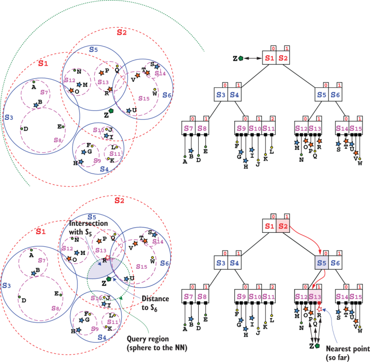
Figure 10.20 Nearest neighbor search. This figure shows the first steps of the call on the root of the tree. (Top) Initially, the search area is a sphere centered at the query point Z, and with infinite radius (although here it’s shown as a circle that includes the whole tree, for consistency). (Bottom) The search traverses the tree, choosing first the closest branches. S5’s border is closer than S6’s, so we visit the former first (although, as you can see, the opposite choice would be the best, but the algorithm can’t know that yet). Normally the distance is computed from a node’s bounding envelope, but since Z intersects both S1 and S2, it first chooses the one whose centroid is closer. The algorithm goes in depth as much as possible, traversing a path to a leaf before back-tracking. Here we show the path to the first leaf: once there, we can update the query region that now is the sphere centered at Z with radius equal to the distance to R, the closest point in S13, which is therefore saved as the best guess for the nearest neighbor.

This simplicity and cleanness are not unexpected. We have done the hard work of the design and creation of the data structure, and now we can enjoy the benefits!

Figure 10.21 Nearest neighbor search. A summary of the next steps in the traversal. Arrows are numbered to reflect the order of the recursive calls. (Top) After visiting S13 and finding R as the best guess for the nearest neighbor, S12 is skipped because it’s outside the update search region. Then the execution backtracks, and we get to S5’s sibling, S6, which still has a non-null intersection with the search region. (Bottom) Fast-forward to the end of the traversal. We need to traverse S1’s branch as well, because Z lies within it. As a matter of fact, the search region intersects another leaf, S10, so we need to traverse a path to it. As you can see, point J is close to being Z’s nearest neighbor, so it’s not unlikely that we would find the true NN in a later call.

Listing 10.19 The nearestNeighbor method for SS-tree

function nearestNeighbor(node, target, (nnDist, nn)=(inf, null))      ❶
  if node.leaf then                                                   ❷
    for point in node.points do                                       ❸
      dist ← distance(point, target)                                  ❹
      if dist < nnDist then                                           ❺
        (nnDist, nn) ← (dist, point)                                  ❺
  else                                    
    sortedChildren ← sortNodesByDistance(node.children, target)       ❻
    for child in sortedChildren do                                    ❼
      if nodeDistance(child, target) < nnDist then                    ❽
        (nnDist, nn) ← nearestNeighbor(child, target, (nnDist, nn))   ❾
  return (nnDist, nn)                                                 ❿

❶ Function nearestNeighbor returns the closest point to a given target. It takes the node to search and the query point. We also (optionally) pass the best values found so far for nearest neighbor (NN) and its distance to help pruning. These values default to null and infinity for a call on the tree root, unless we want to limit the search inside a spherical region (in that case, just pass the sphere’s radius as the initial value for nnDist).

❷ Checks if node is a leaf. Leaves are the only nodes containing points, and so are the only nodes where we can possibly update the nearest neighbor found.

❸ Cycles through all points in this leaf

❹ Computes the distance between current point and target

❺ If that distance is less than the current NN’s distance, we have to update the values stored for the NN and its distance.

❻ If, instead, node is an internal node, we need to cycle through all its children and possibly traverse their subtrees. We start by sorting node’s children from the closest to the furthest with respect to target. As mentioned, a different heuristic than the distance to the bounding envelope can be used here.

❼ Cycles through all children in the order we sorted them

❽ Checks if their bounding envelope intersects with the NN bounding sphere. In other words, if the distance from target to the closest point within child’s bounding envelope is smaller than the pruning distance (nnDist).

❾ If the distance between target and child is smaller than the pruning distance, then it traverses the subtree rooted at child, updating the result.

❿ All that remains is to return the updated values for the best result found so far.

Of the helper methods in listing 10.19, it’s important to spend some time explaining function nodeDistance. If we refer to figure 10.22, you can see why the minimum distance between a node and a bounding envelope is equal to the distance between the centroids minus the envelope’s radius: we just used the formula for the distance between a point and a sphere, taken from geometry.

Figure 10.22 Minimum distance to a bounding envelope. Consider the triangle ZBCB. Then, for the triangular inequality, |CBB|+|BZ|>|ZCB|, but |ZCB|==|ZA|+|ACB| and |ACB|==|CBB| (they are both radii), so ultimately |CBB|+|BZ|>|ZA|+|ACB|⇒|BZ|>|ZA|. Therefore, the minimum distance is the length of segment from Z to SB’s sphere, along the direction connecting its centroid to Z.

We can easily extend the nearest neighbor search algorithm to return the n-th nearest neighbor. Similar to what we did in chapter 9 for k-d trees, we just need to use a bounded priority queue that keeps at most n elements, and use the furthest of those n points as a reference, computing the pruning distance as the distance from this point to the search target (as long as we have found fewer than n points, the pruning distance will be infinity).

Likewise, we can add a threshold argument to the search function, which becomes the initial pruning distance (instead of passing infinity as the default value for nnDist), to also support search in spherical regions. Since these implementations can be trivially obtained, referring to chapter 9 for guidance, we leave them to the readers (for a hint, check the implementation on the book’s repo on GitHub¹⁵).

10.4.2 Region search

Region search will be similar to what we have described for k-d trees—the only difference being how we need to compute the intersection between each node and the search region, besides the structural change due to the fact that points are only stored in leaves.

Listing 10.20 shows a generic implementation of this method for SS-trees that assumes the region passed as argument includes a method to check whether the region itself intersects a hyper-sphere (a node’s bounding envelope). Please refer to section 9.3.6 for a detailed explanation and examples about search on the most common types of regions, and their algebraic meaning.

Listing 10.20 The pointsWithinRegion method for SS-tree

function pointsWithinRegion(node, region)                    ❶
  points ← []                                                ❷
  if node.leaf then                                          ❸
    for point in node.points do                              ❹
      if region.intersectsPoint(point) then                  ❺
        points.insert(point)                                 ❺
  else    
   for child in node.children do                             ❻
      if region.intersectsNode(child) then                   ❼
        points.insertAll(pointsWithinRegion(child, region))  ❽
  return points                                              ❾

❶ Function pointsWithinRegion takes a node on which the search must be performed, as well as the search region. It returns a list of points stored in the subtree rooted at node and lying within the search region (in other words, the intersection between the region and the node’s bounding envelope).

❷ Initializes the return value to an empty list

❸ Checks if node is a leaf

❹ Cycles through all points in the current leaf

❺ If the current point is within the search region, it’s added to the list of results. The onus of providing the right method to check if a point lies in a region is on the region’s class (so regions of different shapes can implement the method differently).

❻ If, instead, node is an internal node, cycles through its children

❼ Checks to see if the search region intersects the current child. Again, the region’s class will have to implement this check.

❽ If there is any intersection (so there might be points in common), we should call this method recursively on the current child, and then add all the results found, if any, to the list of points returned by this method call.

❾ At this point, we can just return all the points we collected in this method call.

10.4.3 Approximated similarity search

As mentioned, similarity search in k-d trees, as well as R-trees and SS-trees, suffers from what is called the curse of dimensionality: the methods on these data structures become exponentially slower with the growth of the number of dimensions of the search space. K-d trees also suffer from additional sparsity issues that become more relevant in higher dimensions.

While using R-trees and SS-trees can improve the balance of the trees and result in better trees and faster construction, there is still something more we can do to improve the performance of the similarity search methods.

These approximate search methods are indeed a tradeoff between accuracy and performance; there are a few different (and sometimes complementary) strategies that can be used to have faster approximate queries:

• Reduce the dimensionality of the objects—Using algorithms such as PCA or Discrete Fourier Transform, it is possible to project the dataset’s object into a different, lower-dimensional space. The idea is that this space will maintain only the essential information to distinguish between different points in the dataset. With dynamic datasets, this method is obviously less effective.

• Reduce the number of branches traversed—As we have seen in the previous section, our pruning strategy is quite conservative, meaning that we traverse a branch if there is any chance (even the slightest) that we can find a point in that branch closer than our current nearest neighbor. By using a more aggressive pruning strategy, we can reduce the number of branches (and ultimately dataset points) touched, as long as we accept that our results might not be the most accurate possible.

• Use an early termination strategy—In this case, the search is stopped when the current result is judged good enough. The criterion to decide what’s “good enough” can be a threshold (for instance, when a NN closer than some distance is found), or a stop condition connected to the probability of finding a better match (for instance, if branches are visited from closer to further with regard to the query point, this probability decreases with the number of leaves visited).

We will focus on the second strategy, the pruning criterion. In particular, we can provide a method that, given a parameter ϵ, called the approximation error, with 0.0 ≤ ϵ ≤ 0.5, guarantees that in an approximated n-nearest neighbor search, the n-th nearest neighbor returned will be within a factor (1+ϵ) from the true n-th nearest neighbor.

To explain this, let’s restrict¹⁶ to the case where n==1, just plain NN search. Assume the approximated NN-search method, called on a point P, returns a point Q, while the real nearest neighbor of P would be another point N≠Q. Then, if the distance between P and its true nearest neighbor N is d, the approximated search distance between P and Q will be at most (1+ϵ)*d.

Guaranteeing this condition is easy. When we prune a branch, instead of checking to see if the distance between the target point and the branch’s bounding envelope is smaller than the current NN distance, we prune unless it is smaller than 1/(1+ϵ) times the NN’s distance.

If we denote with Z the query point, with C current nearest neighbor, and with A the closest point to Z in the branch pruned (see figure 10.21), we have, in fact

So, if the distance of the closest point in the branch is higher than the current NN’s distance over the reciprocal of (1+ϵ), we are guaranteed that the possible nearest neighbor held in the branch is no further than an epsilon factor from our current nearest neighbor.

Of course, there could be several points in the dataset that are within a factor (1+ϵ) from the true nearest neighbor, so we are not guaranteed that we get the second-closest point, or the third, and so on.

However, the probability that these points exist is proportional to the size of the ring region with radii nnDist and nnDist/(1+ϵ), so the smaller we set ϵ, the lower the chances we are missing closer points.

A more accurate estimate of the probability is given by the area of the intersection of the aforementioned ring with the bounding envelope of the node we skip. Figure 10.23 illustrates this idea, and shows the difference between SS-trees, k-d trees, and R-trees: the probability is maximum when the inner radius is just tangent to the area, and a sphere has a smaller intersection, with respect to any rectangle.

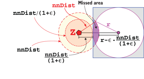
Figure 10.23 The probability of missing j points by using an approximation error is proportional to the intersection of the pruned search area (the ring with radius (ϵ/(1+ϵ))*nnDist) and the bounding envelope of the node intersecting this region, but not the internal sphere with reduced radius. The maximum probability corresponds to a region tangent to the internal sphere. The figure shows how the intersection is smaller for spherical bounding envelopes than for rectangular ones.

If we set ϵ==0.0, then we get back the exact search algorithm as a special case, because nnDist/(1+epsilon) becomes just nnDist.

When ϵ>0.0, a traversal might look like figure 10.24, where we use an example slightly different from the one in figures 10.20 and 10.21 to show how approximate NN search could miss the nearest neighbor.

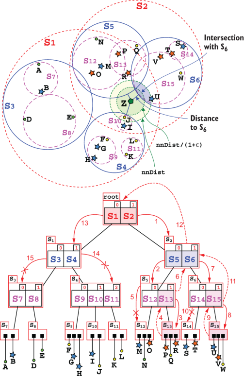
Figure 10.24 Approximated nearest neighbor search. The example is similar (almost identical) to the one in figures 10.20 and 10.21, to allow a close comparison. We show the verbose representation of the tree to make clearer the path followed in traversal. Node S4 contains J, the true NN, whose bit is further away from the query point Z than S5 and S6, and outside the approximated query region (ϵ has been chosen ad hoc, obviously, to cause this condition, in this example, ϵ~=0.25). Arrows are numbered in the order in which they are traversed.

In many domains we can be not just fine, but even happy, with approximate search. Take our example of the search through a dataset of images: Can we really be sure that an exact match is better than an approximate one? If we were working with geographic coordinates—say, on a map—then a factor ϵ difference could have dire consequences (at the very best, taking a longer route would be expensive, but it might get as bad as safety issues). But when the task is finding the dresses that most closely resemble a purchase, then we can’t even guarantee the precision of our metric. Maybe a couple of feature vectors are slightly closer than another pair, but in the end, to the human eye, the latter images look more similar!

So, as long as the approximation error ϵ is not too large, chances are that an approximated result for “most similar image” will be as good as, or maybe better, than the exact result.

The interested reader can find plenty of literature on the topic of approximated similarity search and delve deeper into the concepts that we could only superficially examine here. As a starting point I suggest the remarkable work of Giuseppe Amato.¹⁷

10.5 SS+-tree¹⁸

So far, we have used the original SS-tree structure, as described in the original paper by White and Jain¹⁹; SS-trees have been developed to reduce the nodes overlapping, and in turn the number of leaves traversed by a search on the tree, with respect to R-trees and k-d trees.

10.5.1 Are SS-trees better?

With respect to k-d trees, the main advantage of this new data structure is that it is self-balancing, so much so that all leaves are at the same height. Also, using bounding envelopes instead of splits parallel to a single axis mitigates the curse of dimensionality because unidimensional splits only allow partitioning the search space along one direction at a time.

R-trees also use bounding envelops, but with a different shape: hyper-rectangles instead of hyper-spheres. While hyper-spheres can be stored more efficiently and allow for faster computation of their exact distance, hyper-rectangles can grow asymmetrically in different directions: this allows us to cover a node with a smaller volume, while hyper-spheres, being symmetrical in all directions, generally waste more space, with large regions without any point. And indeed, if you compare figure 10.4 to figure 10.8, you can see that rectangular bounding envelopes fit the data more tightly than the spherical ones of the SS-tree.

On the other hand, it can be proved that the decomposition in spherical regions minimizes the number of leaves traversed.²⁰

If we compare the growth of the volume of spheres and cubes in a k-dimensional spaces, for different values of k, given by these formulas

we can see that spheres grow more slowly than cubes, as also shown in figure 10.25.

And if a group of points is uniformly distributed along all directions and shaped as a spherical cluster, then a hyper-sphere is the type of bounding envelope that wastes the lowest volume, as you can see also for a 2-D space in figure 10.23, where a circle of radius r is inscribed in a square of side 2r. If the points are distributed in a circular cluster, then all the areas between the circle and its circumscribed square (highlighted in figure 10.23) are potentially empty, and so wasted.

Figure 10.25 Volume of spheres (lighter line) and cubes (darker line) for various radii, as a function of the number of dimensions of the search space

Experiments have confirmed that SS-trees using spherical bounding envelopes perform better on datasets uniformly distributed along all directions, while rectangular envelopes work better with skewed datasets.

Neither R-trees nor SS-trees can offer logarithmic worst-case upper bounds for their methods. In the (unlikely, but possible) worst case, all leaves of the tree will be traversed, and there are at most n/m of them. This means that each of the main operations on these data structures can take up to linear time in the size of the dataset. Table 10.1 summarizes their running time, comparing them to k-d trees.

Table 10.1 Operations provided by k-d tree, and their cost on a balanced k-d tree with n elements

Operation	k-d tree	R-tree	SS-tree
Search	O(log(n))	O(n)	O(n)
Insert	O(log(n))	O(n)	O(n)
Remove	O(n1-1/k)a	O(n)	O(n)
nearestNeighbor	O(2k + log(n))a	O(n)	O(n)
pointsInRegion	O(n)	O(n)	O(n)

^a Amortized, for a k-d tree holding k-dimensional points.

10.5.2 Mitigating hyper-sphere limitations

Now this question arises: Is there anything we can do to limit the cons of using spherical bounding envelopes so that we can reap the advantages when we have symmetrical datasets, and limit the disadvantages with skewed ones?

To cope with skewed datasets, we could use ellipsoids instead of spheres, so that the clusters can grow in each direction independently. However, this would complicate search, because we would want to compute the radius along the direction connecting the centroid to the query point, which in the general case won’t lie on any of the axes.

A different approach to reduce the wasted area attempts to reduce the volume of the bounding spheres used. So far we have always used spheres whose center was a group of points’ center of mass, and whose radius was the distance to the furthest point, so that the sphere would cover all points in the cluster. This, however, is not the smallest possible sphere that covers all the points. Figure 10.26 shows an example of such a difference.

Figure 10.26 Difference between the spheres with minimum radius centered at the cluster centroid (left), and the minimum covering sphere (right) for an example set of points.

Computing this smallest enclosing sphere in higher dimensions is, however, not feasible, because the algorithm to compute the exact values for its center (and radius) is exponential in the number of dimensions.

What can be done, however, is computing an approximation of the smallest enclosing sphere, starting with the center of mass of the cluster as an initial guess. At the very high level, the approximation algorithm tries at each iteration to move the center toward the farthest point in the dataset. After each iteration, the maximum distance the point can move is shortened, limited by the span of the previous update, thus ensuring convergence.

We won’t delve deeper into this algorithm in this context; the interested readers can read more about this method, starting, for instance, with this article²¹ by Fischer et al.

For now, we will move to another way we could improve the balancing of the tree: reducing the node overlap.

10.5.3 Improved split heuristic

We saw in section 10.3 that splitting and merging nodes, as well as “borrowing” points/children from siblings, can result in skewed clusters that require bounding envelopes larger than necessary, and increase node overlap.

To counteract this effect, Kurniawati et al., in their work²² on SS+-trees, introduce a new split heuristic that, instead of only partitioning points along the direction of maximum variance, tries to find the two groups such that each of them will collect the closest nearby points.

To achieve this result, a variant of the k-means clustering algorithm will be used, with two constraints:

• The number of clusters will be fixed and equal to 2.

• The maximum number of points per cluster is bound to M.

We will talk in more depth about clustering and k-means in chapter 12, so please refer to section 12.2 to see the details of its implementation.

The running time for k-means, with at most j iterations on a dataset with n points, is O(jkn),²³ where, of course, k is the number of centroids.

Since for the split heuristic we have k==2, and the number of points in the node to split is M+1, the running time becomes O(jdM), compared to O(dM) we had for the original split heuristic described in section 10.3. We can therefore trade off the quality of the result for performance by controlling the maximum number of iterations j. Figure 10.27 shows an example of how impactful this heuristic can be, and why the increase in running time is well worth it.

Figure 10.27 An example of the different partitions produced by the split heuristic in the original SS-tree version (center) and the k-means split heuristic (left). For the original heuristic, the direction of maximum variance was along the y axis. For this example, we assume M==12 and m==6.

Although newer, more complex clustering algorithms have been developed during the years (as we’ll see in chapter 12, where we’ll also describe DBSCAN and OPTICS), k-means is still a perfect match for SS-trees, because it naturally produces spherical clusters, each with a centroid equal to the center of mass of the points in the cluster.

10.5.4 Reducing overlap

The k-means split heuristic is a powerful tool to reduce node overlapping and keep the tree balanced and search fast, as we were reminded at the beginning of last section; however, we can unbalance a node while also deleting points, in particular during merge or when we move a point/child across siblings. Moreover, sometimes the overlapping can be the result of several operations on the tree and involve more than just two nodes, or even more than a single level.

Finally, the k-means split heuristic doesn’t have overlap minimization as a criterion, and because of the intrinsic behavior of k-means, the heuristic could produce results where a node with larger variance might completely overlap a smaller node.

To illustrate these situations, the top half of figure 10.28 shows several nodes and their parents, with a significant overlap.

Figure 10.28 An example where the grandchildren-split heuristic could be triggered and would lower the nodes overlap. The SS-tree in the example has m==2 and M>=5. The k-means split heuristic is run on the points A-L, with k==5. Notice how k-means can (and sometimes will) output fewer clusters than the initial number of centroids. In this case, only four clusters were returned.

To solve such a situation, SS+-trees introduce two new elements:

1. A check to discover such situations.

2. A new heuristic that applies k-means to all grandchildren of a node N (no matter whether they are points or other nodes; in the latter case their centroids will be used for clustering). The clusters created will replace N’s children.

To check the overlap, the first thing we need is the formula to compute the volume of intersections of two spheres. Unfortunately, computing the exact overlap of two hyperspheres, in the generic k-dimensional case, requires not just substantial work and good calculus skills to derive the formulas, but also robust computing resources, as it results in a formula that includes an integral whose computation is clearly expensive enough to cause you to question its usefulness in a heuristic.

An alternative approach is to check whether one of the two bounding envelopes is completely included in the other. Check that the center of one sphere is contained in the other one, and that the distance of the centroid of the smaller sphere is closer than R-r to the centroid of the larger one, where R is the radius of the larger sphere and, as you might expect, r is the radius of the smaller one.

Variants of this check can set a threshold for the ratio between the actual distance of the two centroids and R-r, using it for an approximation of the overlapping volume as this ratio gets closer to 1.

The reorganization heuristic is then applied if the check’s condition is satisfied. A good understanding of k-means is needed to get into the details of this heuristic, so we’ll skip it in this context, and we encourage readers to refer to chapter 12 for a description of this clustering algorithm. Here, we will use an example to illustrate how the heuristic works.

In the example, the heuristic is called on node S1 and the clustering is run on its grandchildren, points A-L. As mentioned, these could also be centroids of other internal nodes, and the algorithm wouldn’t change.

The result is shown in the bottom half of figure 10.28. You might wonder why there are now only four children in node S1: even if k-means was called with k, the number of initial clusters, equal to five (the number of S1’s children), this clustering algorithm could output fewer than k clusters. If at any time during its second step, points assignment, one of the centroids doesn’t get any point assigned, that centroid just gets removed and the algorithm continues with one less cluster.

Both the check and the reorganization heuristic are resource-consuming; the latter in particular requires O(jMk) comparisons/assignments, if j is the number of maximum iterations we use in k-means. Therefore, in the original paper it was recommended to check the overlap situation after splitting nodes, but to apply the reorganization infrequently.

We can also easily run the check when an entry is moved across siblings, while it becomes less intuitive when we merge two nodes. In that case, we could always check all pairs of the merged node’s sibling, or—to limit the cost—just sample some pairs.

To limit the number of times we run the reorganization heuristic and avoid running it again on nodes that were recently re-clustered, we can introduce a threshold for the minimum number of points added/removed on the subtree rooted at each node, and only reorganize a node’s children when this threshold is passed. These methods prove to be effective in reducing the variance of the tree, producing more compact nodes.

But I’d like to conclude the discussion about these variants with a piece of advice: start implementing basic SS-trees (at this point, you should be ready to implement your own version), then profile them within your application (like we did for heaps in chapter 2), and only if SS-trees appear to be a bottleneck and improving their running time would reduce your application running time by at least 5-10%, try to implement one or more of the SS+-tree heuristics presented in this section.

Summary

• To overcome the issues with k-d trees, alternative data structures such as R-trees and SS-trees have been introduced.

• The best data structure depends on the characteristics of the dataset and on how it needs to be used, the dimension of the dataset, the distribution (shape) of the data, whether the dataset is static or dynamic, and whether your application is search-intensive.

• Although R-trees and SS-trees don’t have any guarantee on the worst-case running time, in practice they perform better than k-d trees in many situations, and especially for higher-dimensional data.

• SS+-trees improve the structure of these trees by using heuristics that reduce the number of nodes overlapping.

• You can trade the quality of search results for performance by using approximated similarity searches.

• There are many domains where exact results for these searches are not important, because either we can accept a certain error margin, or we don’t have a strong similarity measure that can guarantee that the exact result will be the best choice.

• An example of such a domain is similarity search in an image dataset.

---

^1. Convolutional Neural Network, a type of deep neural network that is particularly well-suited to process images.

^2. A B-tree is a self-balancing tree optimized for efficiently storing large datasets on disk.

^3. A memory page, or just page.

^4. An attentive reader will remember that we already discussed the branching factor in chapter 2 for d-ary heaps.

^5. See, for instance, https://sqlity.net/en/2445/b-plus-tree/.

^6. The centroid is defined as the center of mass of a set of points, whose coordinates are the weighted sum of the points’ coordinates. If N is a leaf, its center is the centroid of the points belonging to N; if N is an internal node, then we consider the center of mass of the centroids of its children nodes.

^7. Since the height of the tree is at most log_M(n), if m==M/2 (the choice with the largest height) log_M/2(n)~= log_M(n).

^8. As long as it satisfies the requirements for a valid metric: being always non-negative, being null only between a point and itself, being symmetrical, and abiding by the triangular inequality.

^9. Remember: one of the golden rules of clean code is breaking up long, complex methods into smaller ones, so that each method is focused on one goal only.

^10. Assuming a point’s centroid is the point itself. We will also assume points have a radius equal to 0.

^11. Disclaimer: A function that returns a value and has a side effect is far from ideal and not the cleanest design. Using indirect sorting would be a better solution. Here, we used the simplest solution because of limited space, but be advised.

^12. For SS-trees we partition the ordered list of points by selecting the split index for the list, and then each point on the left of the index goes in one partition, and each point on the right in the other partition.

^13. We could reuse search as the first call in delete (and searchClosestLeaf in insert) if we store a pointer to its parent in each node, so that we can climb up the tree when needed.

^14. Assuming you implement this method as a private method. Assertions should never be used to check input, because they can be (and often are, in production) disabled. Checking arguments in private methods is not ideal and must be avoided when they are forwarded from user input. Ideally, you would only use assertions on invariants.

^15. See https://github.com/mlarocca/AlgorithmsAndDataStructuresInAction#ss-tree.

^16. This can easily be extended to n-nearest neighbor by considering the distance of the n-th NN instead.

^17. See Amato, Giuseppe. “Approximate similarity search in metric spaces.” Diss. Technical University of Dortmund, Germany, 2002.

^18. This section includes advanced material focused on theory.

^19. See White, David A., and Ramesh Jain. “Similarity indexing with the SS-tree.” Proceedings of the Twelfth International Conference on Data Engineering. IEEE, 1996.

^20. See Cleary, John Gerald. “Analysis of an algorithm for finding nearest neighbors in Euclidean space.” ACM Transactions on Mathematical Software (TOMS) 5.2 (1979): 183-192.

^21. See Fischer, Kaspar, Bernd Gärtner, and Martin Kutz. “Fast smallest-enclosing-ball computation in high dimensions.” European Symposium on Algorithms. Springer, Berlin, Heidelberg, 2003.

^22. “SS+ tree: an improved index structure for similarity searches in a high-dimensional feature space.” Storage and Retrieval for Image and Video Databases V. Vol. 3022. International Society for Optics and Photonics, 1997.

^23. To be thorough, we should also consider that computing each distance requires O(d) steps, so the running time, if d can vary, becomes O(djkn). While for SS-trees we have seen that it becomes important to keep in mind how algorithms perform when the dimension of the space grows, a linear dependency is definitely good news, and we can afford to omit it (as it is done by convention, considering the dimension fixed) without distorting our result.