In this appendix, we provide a refresher about the RAM model and the renowned big-O mathematical notation, showing you it’s not as bad as you might have heard. Don’t worry; to go through the book you’ll only need a high-level understanding, just the bare minimum to apply it in the algorithm analysis.

B.1 Algorithms and performance

Describing the performance of an algorithm is not a trivial exercise. You might be used to describing the performance of your code in term of benchmarks, and that might seem straightforward, but if you start thinking about how to describe it effectively, so that your findings can be shared and be meaningful to others, then it raises more issues than you initially thought of.

For example, what does performance even mean? It usually implies some kind of measure, so what will it be?

Your first answer might be that you measure the time interval needed to run the algorithm on a certain input. A step further might even be realizing that you might need to average over several inputs, and several runs on the same input, to account for external factors. This would still be a noisy measurement, especially with modern multicore architectures. It’s going to be hard to sandbox your experiments, and both the operating system and background processes will influence the result.

But this is not even the worst part. This result will be largely influenced by the hardware you are running your experiments on, so it won’t have any meaning as an absolute number. You might try to run a benchmark test and compare your algorithm performance to some other known algorithm. Sometimes this technique produces meaningful results, but it doesn’t seem like the way to go, because there would still be too many variables to take into consideration, from the hardware and operating system it’s running on to the type and size of input used in your tests.

Continuing in your reasoning, you can think about counting the instructions that are run. This is probably a good indicator of how much time will be needed to run the whole algorithm, and sufficiently generalizable, right?

Well . . . not quite.

1. Will you count machine instructions? If so, it will not be platform-agnostic.

2. If, instead, you count high-level instructions only, it will heavily depend on the programming language you choose. Scala or Nim can be much more succinct than Java, Pascal, or COBOL.

3. What can be considered an improvement? Is it relevant if your algorithm runs 99 instructions instead of 101?

We could keep going, but you should get the gist by now. The issue here is that we were focusing too much on details that have little importance. The key to get out of this impasse is to abstract out these details: this was obtained by defining a simplified computational model, the RAM model. The latter is a set of basic operations working on an internal random access memory.

B.2 The RAM model

Under the RAM model, a few assumptions hold:

• Each basic operation (arithmetic operations, if, or function call) takes exactly a single one-time step (henceforth just referred to as step).

• Loops and subroutines are not considered simple operations. Instead, they are the composition of many one-time-step operations and consume resources proportional to the number of times they run.

• Each memory access takes exactly one step.

• Memory is considered infinite.

The last point might seem a bit unrealistic, but notice that in this model we make no distinction between accesses to actual cache, RAM, hard drive, or data-center storage. In other words

• For most real-world applications, we can imagine providing the memory needed.

• With this assumption, we can abstract away the details of the memory implementation and focus on the logic.

Under the RAM model, the performance of an algorithm is measured as the number of steps it takes on a given input.

These simplifications allow us to abstract out the details of the platform. For some problems or some variants, we might be interested in bringing some details back. For instance, we can distinguish cache accesses from disk accesses. But in general, this generalization serves us well.

Now that we’ve established the model we’ll use, let’s discuss what we’ll consider to be relevant improvement of an algorithm.

B.3 Order of magnitude

The other aspect we still need to simplify is the way we count instructions. We might decide to count only some kinds of operations like memory accesses. Or, when analyzing sorting algorithms, we can only take into account the number of element swaps.

Also, as suggested, small variations in the number of steps executed are hardly relevant. Rather, we could reason on order of magnitude changes: 2x, 10x, 100x, and so on.

But to really understand when an algorithm performs better than another one on a given problem instance, we need another epiphany: we need to express the number of steps performed as a function of the problem size.

Suppose we are comparing two sorting algorithms, and we state that “on a given test set, the first algorithm takes 100 steps to get to the solution while the second one takes 10.” Does that really help us predict the performance of either algorithm on another problem instance?

Conversely, if we can prove that on an array with n elements, algorithm A needs n * n element swaps, while algorithm B only takes n, then we have a very good way to predict how each of them will perform on input of any size.

This is where big-O notation kicks in. But first, take a look at figure B.1 to get an idea of how the running times for these two algorithms would compare. This chart should make you realize why we would like to stick with algorithm B.

Figure B.1 Visual comparison of the running time of a quadratic algorithm (A) and a linear algorithm (B). The former grows so much faster that, although the y axes shows up to 10 times the max value reached by algorithm B, it only manages to show the plot for algorithm A (the curvy line) up to¹ n~=30.

B.4 Notation

Big-O notation is a mathematical symbolization used to describe how certain quantities grow with the size of an input. Usually it takes the form of a capital o, enclosing an expression within parentheses: something like O(f(n)), hence the name big-O. f(n) here can be any function with input n; we only consider functions on integers, because n usually describes the size of some input.

We are not going to describe big-O notation in detail here; it’s way out of our scope. But there are many textbooks available with in-depth dissertations on the topic.

The main concept you need to remember is that the notation O(f(n)) expresses a bound.

Mathematically, saying g(n) = O(f(n)) means that for any large enough input, there is a real value constant c (whose value does not depend on n), such that g(n) ≤ c * f(n) for every possible value of n (possibly larger than a certain value n0).

For instance, if f(n) = n and g(n) = 40 + 3*n, we can choose c = 4 and n0 = 40.

Figure B.2 shows how these three functions grow with respect to each other. While f(n) is always smaller than g(n), c*f(n) becomes larger than g(n) at some point. To better understand the turning point, we can evaluate the two formulas by substituting actual values for their parameter n. We use the following notation f(1) -> 1 to assert that f(1) evaluates to 1 (in other words, the result of calling f(1) is equal to 1).

For n lower than 40, g(n) will be larger. For n = 30, f(30) -> 120 and g(n) -> 130. Instead, we know that f(40) -> 160 and g(40) -> 160, f(41) -> 164 while g(41) -> 163. For any value greater than 41, 40 + 3 *n <= 4 * n.

Figure B.2 Visual comparison of functions: f(n)=n, g(n) = 40 + 3*n, 4*f(n). While f(n) is always smaller than g(n), 4*f(n) becomes larger than g(n) for sufficiently large values of n.

But don’t forget that the condition g(n) ≤ c * f(n) must hold true for every n ≥ n0. We can’t rigorously prove that by plotting a chart or plugging in (a finite number of) values for n in the formula (see figure B.3 for a counter-example), but we would need to resort to some algebra; nevertheless, plotting the functions can help you get an idea of how they grow and whether you are going in the right direction.

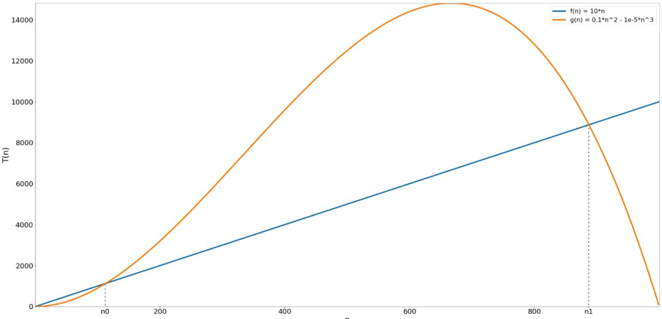
Figure B.3 An example showing why we need to be careful when drawing conclusions. While g(n) is larger than f(n) at n0~=112, this doesn’t hold true for any value of n >n0. In fact, at n1~=887, we have another intersection between the two functions, and after that point f(n) again becomes larger than g(n).

Moving back to our example, if we say that algorithm A is O(n2), it means that T(n) = O(n2), where T(n) is the running time of the algorithm. Or, in other words, algorithm A will never require more than a quadratic number of steps.

The definition for O(n) has some consequences:

• “For any large enough input.” This is a crucial piece. We are interested in how our functions behave when n gets (very) large and we don’t care if for small values of n the inequalities don’t hold. Think, for example, of the functions f(x) = ex and g(x) = e * x. f(x) < g(x) when x is smaller than 1, but for larger values, f(x) grows much faster.

• Constant factors don’t matter: O(n) = O(3 * n) = O(100 * n). You can prove this by choosing the right values for the constant in the previous inequality.

• Some problems require constant time: think about summing the first n integers. With the naïve algorithm, you would need n-1 sums, but with Gauss’ method, you only need one sum, one multiplication and one division, independent of the output.

  To sum this up using a formula, we can write O(c) = O(1) for any positive constant c.

  O(1) denotes a constant running time: in other words, one that does not depend on the input size.

• When summing big-O expressions, the biggest wins: O(f(n) + g(n)) = O(f(n)) if g(n) = O(f(n)). So, if two algorithms are run in sequence, the total running time is dominated by the slowest.

• O(f(n) * g(n)) can’t be simplified unless either function is constant.

Note Often when we give an algorithm running time using big-O notation, we imply that the bound is both lower and upper—unless we explicitly say otherwise. Nevertheless, Θ(f(n)) would be the correct notation for the class of functions whose upper and lower bound is f(n).

Now we have all the tools we need to unequivocally describe algorithms’ performance. You will see this notation in action a lot in the remaining sections of this appendix.

B.5 Examples

If it’s the first time you have seen big-O notation, it’s perfectly normal to feel slightly confused. It takes some time and lots of practice to get used to it.

Let’s see a few examples and try to apply what we described in the previous section in mathematical terms.

Suppose you have 4 numbers you’d like to sum: {1, 3, -1.4, 7}. How many additions will you need? Let’s see:

1 + 3 + (-1.4) + 7

It looks like you can do with three additions. What about if we have to sum 10 numbers? You can easily verify that we need nine. Can we generalize this number of operations for any size of the input? Yes, we can, as it’s easy to prove that we always need n-1 additions to sum up n numbers.

So, we can say that summing up the elements of a list of n numbers (asymptotically) requires O(n) operations. If we denote with T(n) the number of operations needed, we can say that T(n) = O(n).

Let’s consider two slight variations:

• We sum the first five elements of a list twice, and the other elements once.

• We sum the squares of the elements.

In the first case, if our list is {1, 3, -1.4, 7, 4, 1, 2}, we have

1 + 3 + (-1.4) + 7 + 4 + 1 + 2 + 1 + 3 + (-1.4) + 7 + 4

You can see the repeated elements underlined in this formula. So, for n=7, we need 11 operations.

In general, we will need n+4 operations, and T1(n) = n+4.

Is it true that T1(n) = O(n)? Let’s go back to our definition. We need to find two constants, an integer n0 and a real number c, such that

T1(n) ≤ c * n for each n > n0
⇔
n + 4 ≤ c * n for each n > n0 
⇔
c ≥ 1 + 4/n for each n > n0 

Since 4/n decreases when n grows, we can choose c=2 and n0=4, or, say, c=100 and n₀=1, and the inequality will be satisfied.

The same is true if we consider summing squares: for n numbers, we will need n multiplications (or squarings) and n-1 sums, so T2(n) = 2n-1.

We can prove that T2(n) = O(n) by choosing c=2.5 and n0=1.

Now, we could also say that T1(n) = O(n2). We leave it as an exercise for you to find appropriate values for c and n0. However, this bound would not be strict: in other words, there exist other functions of n such that T1(n) ≤ f(n) < O(n2) for n large enough.

Likewise, we could also say that T1(n) = O(n1000). That would certainly be true, but how helpful would it be knowing that our algorithm takes less than the age of the universe on a small input?²

As you might suspect, we are usually interested in strict bounds. While this is true and expected, and for our summation examples it seems trivial to prove that the O(n) bound is strict, you might be surprised to learn that there are some algorithms for which we don’t know what the stricter bound is, or at least we can’t prove it.

As a final example, let’s consider the task of enumerating all the couples of numbers in a list, regardless of their order. For instance, given the list {1, 2, 3}, we have the pairs (1,2), (1,3), (3,2).

It turns out that the number of unordered pairs for n elements is T3(n) = n * (n-1) / 2:

T3(n) = n * (n-1) / 2 ≤ 1*n2 for n > 1

Thus we can say T3(n) = O(n2). This time, the quadratic bound is also a strict bound, as shown in figure B.4.

Figure B.4 Visual comparison of functions: f(n)=n*(n-1), g(n) = n2. The latter is always larger for any positive value of n.

---

^1. In this context, and for the rest of the book, ~= means “approximately equal to.”

^2. This might be useful if we need to prove that an algorithm will actually run in finite time. But with real-world applications, it’s usually of little practical use.