CHAPTER 10
ML DETECTION TECHNIQUES FOR SISO CHIPLESS RFID TAGS
10.1 INTRODUCTION
Research on chipless radio frequency identification (RFID) systems are mainly emphasizing on improving the RFID reader architecture and the chipless tag design. As a result, tag detection techniques are overshadowed, hence they are using primitive signal processing techniques. The main focus of this chapter is to improve the signal processing techniques using the same reader architecture and tag design. Therefore, the proposed tag detection techniques are compatible with the existing RFID systems. The improvements are expected in successful tag detection rate and the tag reading range.
The existing chipless signal processing techniques for tag detection is as primitive as threshold-based detection. Maximum likelihood (ML)-based detection techniques have shown improved performances in communication systems over primitive techniques such as threshold-based detection techniques. The motivation for this work is to apply the ML detection techniques for chipless RFID tag detection so that the existing RFID systems would produce better results in terms of the detection error rate (DER) and the reading range.
The rest of the chapter is organized as follows. First, the theory behind deriving four ML expressions for a single-input single-output (SISO)-based chipless RFID system is presented. The different expressions are derived based on the availability of the channel information (known or unknown channel) and real or complex signal processing. Then, a computationally feasible tag detection technique is presented so that the detection technique can be implemented on a portable RFID reader. Next, the detection techniques are implemented in MATLAB and its results are compared. Finally, the original contribution and a discussion on each detection technique are presented in the conclusion section.
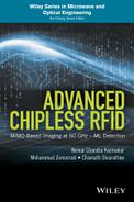
The system models presented in the chapter are for frequency-domain-based chipless RFID tags. However, the models are based on either signal using time-domain samples or frequency-domain samples. Hence, the system models presented can be categorized into two sections as shown in Figure 10.1.
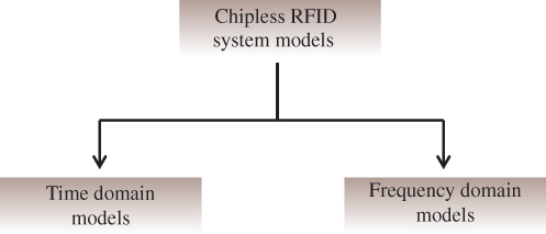
Figure 10.1 RFID system models.
10.2 SYSTEM MODELS–TIME DOMAIN
A multiresonator-based chipless RFID system consists of three main components, namely, a reader, a tag, and the middleware as shown in Figure 10.2. The RFID reader generates an interrogating signal and transmits toward the tag using a transmitting antenna (![]() ). The interrogating signal will be received by the tag using its dedicated receiving antenna (
). The interrogating signal will be received by the tag using its dedicated receiving antenna (![]() ), which has the same polarization as the transmitting antenna of the reader. Then the received signal propagates via a frequency modulation circuit that comprises a cascade of spiral resonators. Depending on the resonator combinations (presence and absence of resonators), a unique tag response is available at the end of the microstrip line. This process is called tag modulation from here onward. Then, the tag response will be transmitted using the dedicated transmitting antenna of the tag (
), which has the same polarization as the transmitting antenna of the reader. Then the received signal propagates via a frequency modulation circuit that comprises a cascade of spiral resonators. Depending on the resonator combinations (presence and absence of resonators), a unique tag response is available at the end of the microstrip line. This process is called tag modulation from here onward. Then, the tag response will be transmitted using the dedicated transmitting antenna of the tag (![]() ). The polarization of the transmitting antennas is orthogonal to that of the receiving antenna of the tag. The transmitted tag response is received at the reader using antennas having matching polarity. This careful selection of the antenna configuration limits any unwanted cross-coupling between antennas.
). The polarization of the transmitting antennas is orthogonal to that of the receiving antenna of the tag. The transmitted tag response is received at the reader using antennas having matching polarity. This careful selection of the antenna configuration limits any unwanted cross-coupling between antennas.
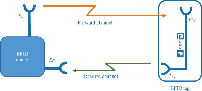
Figure 10.2 Overview of chipless RFID system.
Next, the system is modeled using a number of system models in the following sections.
10.2.1 System Model I–Real Signals
The system described in Figure 10.2 is modeled first using the following simple signal model. Later, more assumptions are relieved and a comprehensive analysis is performed so that the new models closely describe the real system.
The signals considered in System Model I are assumed to be real signals, meaning the received signal is directly sampled at a very high rate. First, the interrogating signal transmitted from the RFID reader reaches the tag through the forward channel as shown in Figure 10.2. Then the signal received by the tag is modulated by the resonator combination present in the tag. ![]() is defined as this resultant signal available for transmitting back toward the reader.
is defined as this resultant signal available for transmitting back toward the reader. ![]() is a unique tag response for a given tag
is a unique tag response for a given tag ![]() and it is a vector having a length of
and it is a vector having a length of ![]() .
. ![]() is then transmitted from the tag to the RFID reader via the reverse channel as shown in Figure 10.2.
is then transmitted from the tag to the RFID reader via the reverse channel as shown in Figure 10.2.
Both the forward and reverse channels are in short range with a strong line of sight. The channels are assumed to be real and known constants. Mixing with the forward channel, tag modulation and mixing with the reverse channel happen in a cascaded manner. As a result, the product of both channels can be represented using a real constant ![]() . The received signal at the reader is added with noise (
. The received signal at the reader is added with noise (![]() ) produced by the receiver circuit at the RFID reader. The resultant signal is called
) produced by the receiver circuit at the RFID reader. The resultant signal is called ![]() and can be represented using Equation (10.1)
and can be represented using Equation (10.1)
When the RFID reader transmits the interrogating signal, it is first received by the receiving antenna of the tag. Then the signal is modulated by the tag and transmitted back toward the RFID reader. ![]() includes both the resonator response as well as the noise introduced by the tag antennas. Therefore,
includes both the resonator response as well as the noise introduced by the tag antennas. Therefore, ![]() is actually dependent on the tag combination. However, the amplitude of the noise added by the receiving antenna of the RFID reader is much higher than the noise added by the tag antennas. This happens due to the close proximity of the transmitter and receiver electronics of the reader to the reader antenna. Also, the reader antenna is expected to have a higher gain compared to the tag antennas. Therefore, it may also pick more surrounding noises. Hence, noise presented in
is actually dependent on the tag combination. However, the amplitude of the noise added by the receiving antenna of the RFID reader is much higher than the noise added by the tag antennas. This happens due to the close proximity of the transmitter and receiver electronics of the reader to the reader antenna. Also, the reader antenna is expected to have a higher gain compared to the tag antennas. Therefore, it may also pick more surrounding noises. Hence, noise presented in ![]() can be neglected and
can be neglected and ![]() can be treated as the pure tag response. The noise presented at the received signal
can be treated as the pure tag response. The noise presented at the received signal ![]() is only due to the noise added at thereader. Therefore, noise
is only due to the noise added at thereader. Therefore, noise ![]() added at the reader can be assumed to be independent of the tag response
added at the reader can be assumed to be independent of the tag response ![]() . In addition, individual time samples of
. In addition, individual time samples of ![]() vector is assumed to follow an independent and identical Gaussian distribution (i.i.d.) with zero mean and a variance of
vector is assumed to follow an independent and identical Gaussian distribution (i.i.d.) with zero mean and a variance of ![]() . As a result, the distributions of
. As a result, the distributions of ![]() and
and ![]() can be derived as in Equation (10.2).
can be derived as in Equation (10.2).

where ![]() is the identity matrix with
is the identity matrix with ![]() dimensions.
dimensions.
Since ![]() and
and ![]() are independent from each other and
are independent from each other and ![]() follows an i.i.d., the probability of receiving
follows an i.i.d., the probability of receiving ![]() given that
given that ![]() has been transmitted can be calculated as follows:
has been transmitted can be calculated as follows:

![]() in Equation (10.3) is the conditional probability of receiving the
in Equation (10.3) is the conditional probability of receiving the ![]() th time sample of
th time sample of ![]() , given
, given ![]() th time sample of tag response
th time sample of tag response ![]() .
. ![]() can be calculated using the well-known probability density function (pdf) of Gaussian distribution as shown in Equation (10.4).
can be calculated using the well-known probability density function (pdf) of Gaussian distribution as shown in Equation (10.4).
Using Equations (10.3) and (10.4), ![]() can be calculated as follows:
can be calculated as follows:

Equation (10.5) can be represented in vectorized form as below. ![]() is the Hermitian transpose.
is the Hermitian transpose.
The received signal, ![]() and all the tag combinations,
and all the tag combinations, ![]() are used to evaluate probabilities given by Equation (10.6). The tag combination
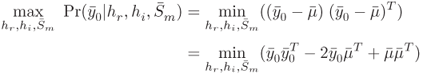
are used to evaluate probabilities given by Equation (10.6). The tag combination ![]() producing highest probability is selected to be the detected tag,
producing highest probability is selected to be the detected tag, ![]() . Therefore,
. Therefore, ![]() is maximized over all possible
is maximized over all possible ![]() combinations for tag detection as follows:
combinations for tag detection as follows:
In Equation (10.6), only the ![]() component is varying with
component is varying with ![]() . Hence, the detector proposed for this model simplifies to Equation (10.8).
. Hence, the detector proposed for this model simplifies to Equation (10.8).
The optimization given by Equation (10.8) performs the tag detection. Under these assumptions, the detector for the proposed signal model is the same as the minimum distance detector. Tag detector used in this section assumes the perfect channel knowledge and both the channel and received signals are considered to be real, even though in reality a typical RFID reader may perform I/Q demodulation hence dealing with complex signals. We release that assumption on next sections by allowing signals to be having both real and imaginary components.
The proposed signal models under different scenarios is listed in Figure 10.3. Signal model II still assumes perfect channel knowledge; however, it utilizes the information available in both the amplitude and phase for decision making. Signal model III needs to know only the statistical properties of the channel, while the actual channel realization is not required for decision making. In signal model IV, the channel is assumed to be unknown and a joint optimization on both the channel and tag type detection is performed. Signal V is derived for an existing chipless RFID system that utilizes only the power magnitudes of the backscattered tag response.

Figure 10.3 Proposed signal models.
10.2.2 System Model II–Complex Signals
The signal model considered in this section is very similar to the System Model I discussed in the previous section. The same assumptions in System Model I apply; however, both the channels and all signals are treated as complex signals. Therefore, I/Q demodulation is implemented at the RFID reader, which is the case for some of the existing RFID readers. As a result, the readers no longer need very high sampling rates and only sample the baseband signals for I & Q. For such a reader, the received signal is called ![]() and can be represented using Equation (10.9)
and can be represented using Equation (10.9)
The product of the forward and reverse channels ![]() is assumed to be known and the signals considered in this model are all complex numbers. They can be represented using real and imaginary quantities for computation simplicity as follows:
is assumed to be known and the signals considered in this model are all complex numbers. They can be represented using real and imaginary quantities for computation simplicity as follows:
Therefore, the received signal can be written as

The noise ![]() added at the reader can be assumed to be independent of the filter response
added at the reader can be assumed to be independent of the filter response ![]() . In addition, real and imaginary components of individual time samples of
. In addition, real and imaginary components of individual time samples of ![]() vector are assumed to follow an independent and identical Gaussian distribution (i.i.d.) with zero mean and a variance of
vector are assumed to follow an independent and identical Gaussian distribution (i.i.d.) with zero mean and a variance of ![]() .
.
A new vector, ![]() having only real values is created using
having only real values is created using ![]() and
and ![]() as follows:
as follows:
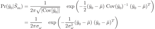
Mean and covariance of ![]() can be calculated as follows:
can be calculated as follows:

![]() in Equation (10.13) is the identity matrix with a dimension of
in Equation (10.13) is the identity matrix with a dimension of ![]() . Using the statistical properties calculated in Equation (10.13) the distribution of the real vector,
. Using the statistical properties calculated in Equation (10.13) the distribution of the real vector, ![]() can be represented as follows:
can be represented as follows:
Similar to the previous sections, the probability of receiving ![]() given that
given that ![]() has been transmitted can be calculated as follows:
has been transmitted can be calculated as follows:
Similar to the previous detectors, Equation (10.14) is evaluated for all the possible tag combinations and the one with the highest probability is taken as the detector output. However, it can be seen that the detector can be further simplified to minimizing the ![]() component. Therefore, the objective function of the detector can be represented as follows:
component. Therefore, the objective function of the detector can be represented as follows:
Under the assumptions followed for the proposed signal model, the optimum detector is the same as the minimum distance detector. However, ![]() and
and ![]() can be calculated using Equations (10.12) and (10.13), respectively. Tag detector used in this section assumes the perfect channel knowledge and both the channel and received signals are considered to be complex, which means in reality the RFID reader performs I/Q modulation/demodulation. However, the expression in Equation (10.15) needs only real number calculations, hence lowers the computation complexity. In the following section, we assume perfect channel knowledge is no longer available. However, statistical properties of the channel are assumed to be available while I/Q modulation/demodulation is assumed to be performed at the RFID reader.
can be calculated using Equations (10.12) and (10.13), respectively. Tag detector used in this section assumes the perfect channel knowledge and both the channel and received signals are considered to be complex, which means in reality the RFID reader performs I/Q modulation/demodulation. However, the expression in Equation (10.15) needs only real number calculations, hence lowers the computation complexity. In the following section, we assume perfect channel knowledge is no longer available. However, statistical properties of the channel are assumed to be available while I/Q modulation/demodulation is assumed to be performed at the RFID reader.
10.2.3 System Model III - Channel with a Known Distribution
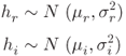
The signal model discussed here assumed that the channel is no longer known. However, the statistical properties of the product of forward and reverse channels are approximated by a Gaussian distribution with a known mean and a variance. Similar to previous models, the channel is assumed to be constant throughout each tag reading. In addition, both the channel and the signals considered in this model are assumed to be complex, meaning I/Q modulation is performed at the RFID reader. Then the received signal can be modeled as
For computation simplicity, the complex channel (![]() ) and the noise (
) and the noise (![]() ) can be represented using two real components as follows:
) can be represented using two real components as follows:
Similar to previous signal models, ![]() is the signal transmitted by the tag and
is the signal transmitted by the tag and ![]() is the noise added at the receiver that is independent of
is the noise added at the receiver that is independent of ![]() and each noise sample follows an independent and identical Gaussian distribution. The statistical properties of the real and imaginary components of the noise (
and each noise sample follows an independent and identical Gaussian distribution. The statistical properties of the real and imaginary components of the noise (![]() and
and ![]() ) is given by Equation (10.16).
) is given by Equation (10.16).

It is assumed that both the real and imaginary components of noise are having the same statistical properties. Next, the product of forward and reverse channels ![]() is assumed to have Gaussian distributions for the real and imaginary components as shown in Equation (10.17).
is assumed to have Gaussian distributions for the real and imaginary components as shown in Equation (10.17).
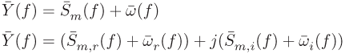
Then the real and imaginary components of the received signal ![]() can be represented using the following relationship:
can be represented using the following relationship:
A new real vector, ![]() is created using
is created using ![]() and
and ![]() as follows:
as follows:
The statistical properties of ![]() and
and ![]() are examined next. It can easily be seen that they too follow a Gaussian distribution. The mean of
are examined next. It can easily be seen that they too follow a Gaussian distribution. The mean of ![]() and
and ![]() is given by Equation (10.20).
is given by Equation (10.20).

Covariances of ![]() and
and ![]() can be calculated using the following formula:
can be calculated using the following formula:
After some calculations, it can be shown that the covariances of ![]() and
and ![]() are as follows:
are as follows:

Therefore, the distribution of ![]() and
and ![]() can be listed as follows:
can be listed as follows:

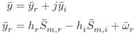
Using Equations (10.19) and (10.22), it can be concluded that ![]() has a multivariate Gaussian distribution with a dimension of 2. The mean of
has a multivariate Gaussian distribution with a dimension of 2. The mean of ![]() can be written as
can be written as
The covariance of ![]() can be calculated as follows:
can be calculated as follows:
After some calculations, it can be seen that ![]() simplifies to
simplifies to

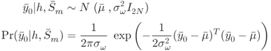
Then the conditional probability on receiving ![]() given that
given that ![]() has been transmitted is given by Equation (10.25):
has been transmitted is given by Equation (10.25):
Similar to previous models, now the probability calculated in Equation (10.25) is maximized over all possible tag combinations, ![]() :
:
In this model, the product of the forward and reverse channels is modeled using a Gaussian distribution. In the next model, we assume no channel information is available. As a result, it is a joint optimization problem of deciding both the channel and the tag combination.
10.2.4 System Model IV–Unknown Channel
In this model, we assume no channel knowledge is available to the RFID reader. In addition, signals considered here are complex, meaning I/Q modulation/ demodulation is utilized at the reader. It is assumed that the product of the forward and reverse channels, ![]() , is an unknown complex number and is a constant during the interrogation time. Then the received signal
, is an unknown complex number and is a constant during the interrogation time. Then the received signal ![]() can be written as
can be written as
For computation simplicity, the complex channel and the noise can be represented using two real components as follows:
Then the received signal ![]() can be represented using the real and imaginary components similar to previous models.
can be represented using the real and imaginary components similar to previous models.

From Equation (10.28), it can be clearly seen that conditional probability of receiving ![]() and
and ![]() given
given ![]() and
and ![]() has a Gaussian distribution. Their statistical properties can be calculated as follows:
has a Gaussian distribution. Their statistical properties can be calculated as follows:

A vector (![]() ) containing real values is created by stacking
) containing real values is created by stacking ![]() and
and ![]() on a row vector as follows:
on a row vector as follows:
Similar to ![]() and
and ![]() , when both the channel
, when both the channel ![]() and the tag combination
and the tag combination ![]() are given, the conditional probability of receiving
are given, the conditional probability of receiving ![]() is having a Gaussian distribution. The mean is given by
is having a Gaussian distribution. The mean is given by
In order to derive an expression for the conditional probability, covariance has to be calculated. The following formulas show how to calculate the covariance:

Then the conditional probability of receiving ![]() given
given ![]() and
and ![]() can be calculated as in Equation (10.32):
can be calculated as in Equation (10.32):
The probability given in Equation (10.32) is maximized over all possible combinations of ![]() and
and ![]() . Therefore, this is a joint optimization problem.
. Therefore, this is a joint optimization problem.
10.2.5 Joint Optimization of  and Tag Type
![]() is calculated using Equation (10.31). However, there are infinitely large number of combinations for
is calculated using Equation (10.31). However, there are infinitely large number of combinations for ![]() and
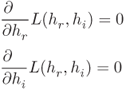
and ![]() ; hence, it is not computationally feasible. A feasible solution would be to first find the optimum channel for a given tag combination. Then the given tag combination response and the optimum channel are used for calculating the conditional probability given in Equation (10.32). Then the same process is repeated for all possible tag combinations, similar to previous detectors, to calculate the highest probability. Next, calculating the optimum channel for a given tag combination is discussed.
; hence, it is not computationally feasible. A feasible solution would be to first find the optimum channel for a given tag combination. Then the given tag combination response and the optimum channel are used for calculating the conditional probability given in Equation (10.32). Then the same process is repeated for all possible tag combinations, similar to previous detectors, to calculate the highest probability. Next, calculating the optimum channel for a given tag combination is discussed. ![]() is defined as follows:
is defined as follows:
For optimum ![]() and
and ![]() , following conditions have to be satisfied:
, following conditions have to be satisfied:
Using Equation (10.31), it can be shown that

Using the relationships in Equations (10.34)(10.35)(10.36), the optimum channel ![]() and
and ![]() for a given
for a given ![]() can be derived as follows:
can be derived as follows:

The optimum channel estimates obtained from Equation (10.37) are used to calculate the optimum ![]() (
(![]() ). Equations (10.31) and (10.37) yield
). Equations (10.31) and (10.37) yield
Then, the new optimization problem reduces to
In this model, no channel information is available to the reader, and the only assumption is that the channel is static during the short interrogation time period. The tag detector derived in the model uses the received signal at the RFID reader and all the possible tag responses to determine both the channel and the tag combination that provides the highest probability.
All the four signal models discussed in this section are based on time-domain signal samples [1]. Some of the existing RFID readers work based on frequency-domain samples. The following section discusses the tag detectors that canwork based on frequency-domain signal samples.
10.3 SYSTEM MODELS–FREQUENCY DOMAIN
Chipless RFID readers are based on either time-domain tags [2–4] or frequency-domain tags [5–11]. Time-domain tags encode the information in time samples of the signal leaving a unique time signature, whereas the frequency-domain tags encode information in the frequency samples of the signal leaving a unique frequency-domain signature. Therefore, it is important to examine the tag detection techniques for the frequency-domain-based chipless RFID tags. There is another very important benefit of using frequency-domain tags. Tag detectors derived for time-domain-based tags have a high computational complexity. However, frequency-domain-based tag detection can be achieved with relatively a lower computational complexity as explained in Chapter 11 in detail. The rest of this section describes five tag detection techniques for frequency-based chipless RFID tags.
10.3.1 System Models I–IV
The tag detectors derived for time-domain chipless RFID tags are first revisited briefly. The signal model used in all the four detectors is as follows:
10.3.1.1 Model I
In model I, channel ![]() is a known real constant. Noise is having a zero mean normal distribution with a covariance
is a known real constant. Noise is having a zero mean normal distribution with a covariance ![]() . Then the probability distribution function of receiving
. Then the probability distribution function of receiving ![]() given that
given that ![]() has been transmitted is given by Equation (10.6). If Fourier transformation is performed on Equation (10.40), the result is shown as follows:
has been transmitted is given by Equation (10.6). If Fourier transformation is performed on Equation (10.40), the result is shown as follows:
![]() is the Fourier transform of the received signal
is the Fourier transform of the received signal ![]() .
. ![]() and
and ![]() are the Fourier transforms of the
are the Fourier transforms of the ![]() th tag response
th tag response ![]() and the noise
and the noise ![]() , respectively. Fourier transform is a unitary transformation. Therefore, the statistical properties of the signals should remain the same. As a result, the probability distribution function of receiving
, respectively. Fourier transform is a unitary transformation. Therefore, the statistical properties of the signals should remain the same. As a result, the probability distribution function of receiving ![]() given that
given that ![]() has been transmitted is the same as Equation (10.6). Therefore, the frequency-domain-based chipless RFID tag detector for system model I can be derived using the frequency samples of the signal as follows:
has been transmitted is the same as Equation (10.6). Therefore, the frequency-domain-based chipless RFID tag detector for system model I can be derived using the frequency samples of the signal as follows:
10.3.1.2 Model II
Similarly, frequency-domain chipless RFID tag detector for system model II can be derived as follows:
Similar to the previous model, ![]() is the Fourier transformation of
is the Fourier transformation of ![]() .
. ![]() and
and ![]() are the Fourier transformations of
are the Fourier transformations of ![]() in Equation (10.12) and
in Equation (10.12) and ![]() in Equation (10.13), respectively.
in Equation (10.13), respectively.
10.3.1.3 Model III
The statistical properties of the signal model III too remain the same, hence the tag detector in frequency domain is given by

![]() and
and ![]() are the Fourier transformations of
are the Fourier transformations of ![]() in Equation (10.23) and
in Equation (10.23) and ![]() in Equation (10.24), respectively.
in Equation (10.24), respectively.
10.3.1.4 Model IV
Similar to previous three models, statistical properties of the detector in signal model do not change with the Fourier transform. Therefore, the tag detector for signal model IV can be written as
![]() and
and ![]() are the Fourier transformations of
are the Fourier transformations of ![]() in Equation (10.30) and
in Equation (10.30) and ![]() in Equation (10.38), respectively.
in Equation (10.38), respectively.
It is clear that the frequency samples of the signal can be used to detect tags using the same detectors derived for the time-based models. It is true that the frequency signature of the frequency-domain tags can be seen in Fourier transformation of the time-domain signal. However, there are chipless RFID readers that work on the power spectral density of the signal, rather than Fourier transformation. In the following section, a tag detector is derived for a power-based chipless RFID reading method.
10.3.2 System Model V – Power Magnitudes
There are chipless RFID readers that operate based on the power measurements rather than on voltage samples. In these readers, a narrow-banded sinusoidal waveform is transmitted as the interrogating signal and the magnitude of the tag response is compared with the transmitted signal using a gain detector. Then the frequency of the narrow-banded interrogating signal is swept across the frequency of interest and the frequency signature of the tag is obtained.
The frequency signature obtained in this method requires a lesser sampling rate at the reader compared to the frequency signature obtained using the Fourier transformation performed on time-domain-based measurements. In addition, the narrow-banded signals are subjected to lesser noise, which could lead to better tag reading reliability.
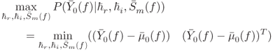
System Model V describes an existing chipless RFID reader developed at Monash Microwave, Antenna, RFID and Sensor Laboratory (MMARS) under Australian Research Council's Linkage Project Grant: LP0991435: Backscatter-based RFID system capable of reading multiple chipless tags for regional and suburban libraries. The reader works on power magnitude of the received tag response. The application assumes a fixed distance between the reader and the tags, and at short distances such as 15 cm, the line-of-sight component dominates over any multipaths. Therefore, the channel undergoes a very slow variation with respect to time. During the calibration phase, all possible tag responses are measured and recorded for the given distance between the reader and the tags. The recorded tag responses are used with the likelihood-based detector derived as follows.
If the Fourier transformation of the tag response is ![]() and the Fourier transformation of the noise added at the reader is
and the Fourier transformation of the noise added at the reader is ![]() , then the Fourier transformation of the received signal at the reader is given by
, then the Fourier transformation of the received signal at the reader is given by ![]() . Then
. Then ![]() is separated into real and imaginary components as shown in Equation (10.46):
is separated into real and imaginary components as shown in Equation (10.46):
As shown in Section 10.3.1, the statistical properties of ![]() is the same as its time-domain samples. Then the power magnitude
is the same as its time-domain samples. Then the power magnitude ![]() of the frequency-domain samples are given by
of the frequency-domain samples are given by
Statistical properties of ![]() and
and ![]() can be written as follows:
can be written as follows:
Then the real (![]() ) and imaginary (
) and imaginary (![]() ) components of
) components of ![]() are defined as follows:
are defined as follows:

The statistical properties of ![]() and
and ![]() can be derived as shown in Equation (10.47).
can be derived as shown in Equation (10.47).
Assuming independence between individual samples of each ![]() and
and ![]() , the probability of receiving
, the probability of receiving ![]() given that
given that ![]() and
and ![]() had been transmitted is given by Equation (10.48).
had been transmitted is given by Equation (10.48). ![]() is the
is the ![]() sample of the corresponding vector.
sample of the corresponding vector.

It is clear that ![]() and
and ![]() are independent. As a result,
are independent. As a result, ![]() has a noncentral chi-square distribution with
has a noncentral chi-square distribution with ![]() being the noncentrality parameter and
being the noncentrality parameter and ![]() being the degree of freedom, which is 2.
being the degree of freedom, which is 2. ![]() for
for ![]() th sample can be calculated as follows:
th sample can be calculated as follows:

Then ![]() can be expressed as follows:
can be expressed as follows:

![]() is the modified Bessel function of the first kind. The above expression can be simplified using
is the modified Bessel function of the first kind. The above expression can be simplified using ![]() and assuming the variance for both real and imaginary noise components is the same (
and assuming the variance for both real and imaginary noise components is the same (![]() ). Then,
). Then,
Using Equations (10.48) and (10.51), ![]() can be calculated as follows:
can be calculated as follows:

![]() in Equation (10.52) is the energy of the selected tag response
in Equation (10.52) is the energy of the selected tag response ![]() defined as
defined as
Then the probability calculated in Equation (10.52) is maximized over ![]() and
and ![]() to detect the most likelihood tag combination.
to detect the most likelihood tag combination.
The tag detection technique developed in this section is used with an existing chipless RFID reader. During the calibration phase, the tag responses for all possible combinations are recorded. Then, the above detection technique is used to detect a random tag.
So far in the chapter, several tag detection techniques have been derived based on both time-domain samples and frequency-domain samples. In order to test these detection techniques comprehensively, a MATLAB simulation is performed, which is explained in the following section.
10.4 SIMULATIONS
The validity of the above tag detection techniques is verified using MATLAB and Computer Simulation Technology (CST) simulations. The steps carried out in the simulation are given in Figure 10.4. First, an interrogating signal was generated to provide a flat frequency response in the 2.2–2.6 GHz frequency range. Four resonators were designed using CST with resonating frequencies as shown in Table 10.1. The resonance frequencies were selected as 100 MHz apart following the specifications provided in Ref. [5]. Then the combinations of resonators were placed beside a microstrip line to cover all possible tag IDs. One end of the microstrip line containing bandstop filters is fed with the interrogating signal and the tag responses are collected at the other end. These collected tag responses were saved in a lookup table for the algorithms to be used later. More details about the tag design are available in Chapter 9.

Figure 10.4 Flowchart of the MATLAB simulation in conjunction with CST full-wave EM solver simulation.
Table 10.1 Simulation Parameters
| Parameter | Value |
| Center frequency | 2.4 GHz |
| Total bits encoded in a tag | 4 bits |
| Flat frequency response | 400 MHz |
| Bandstop filter attenuation | 10 dB |
| Bandstop filter 3 dB bandwidth | 40 MHz |
| Guard-band | 60 MHz |
| Resonance frequency set 1 (MSB to LSB) | [2.2, 2.3, 2.4, 2.5] GHz |
| Resonance frequency set 2 (MSB to LSB) | [2.34, 2.38, 2.42, 2.46] GHz |
| Resonance frequency set 3 (MSB to LSB) | [22.5, 23.5, 24.5, 25.5] GHz |
| Channel mean | 0.4 |
| Channel standard deviation | 0.1 |
| Number of iterations | Up to 10,000,000 |
Then the tag responses were fed through a channel that is given by the product of the forward and reverse channels of the RFID system. Depending on the detection technique, the channel values were selected to be a known constant or a variable with a known or unknown statistical distribution. Finally, noise was added to the resultant signal according to the specified signal-to-noise ratio (SNR).
SNR was calculated compared to the average power of all the tag combinations. It can be summarized as follows:
| – | interrogating signal | |
| – | forward channel |
| – | reverse channel | |
| – | product of forward and reverse channels | |
| – | impulse response of the |
|
| – | ||
| – | received signal | |
| – | noise added at the reader. |
Then the received signal can be represented using Equation (10.55).

The power of each tag response was calculated and averaged to obtain the average power of a given tag response. For example, 2-bit tags have four different tag responses (![]() ) and power of each tag response is calculated and averaged to obtain the average power of 2-bit tag responses. Then the average tag response power was multiplied using the channel to calculate the average signal power available at the reader. For a given SNR, noise power was calculated using this available signal power.
) and power of each tag response is calculated and averaged to obtain the average power of 2-bit tag responses. Then the average tag response power was multiplied using the channel to calculate the average signal power available at the reader. For a given SNR, noise power was calculated using this available signal power.
MATLAB simulation parameters are outlined in 10.1. Four bandstop filters are used, and most significant bit (MSB) corresponds to the lowest resonance frequency and least significant bit (LSB) to the highest.
I/Q demodulation was performed with the received signal at the RFID reader. Then, the two output time-domain signal vectors were used to evaluate likelihood expressions for each detection technique. In order to verify their frequency-domain performances the time-domain vectors were converted using fast Fourier transform (FFT). Then, these frequency-domain samples were used for tag detection.
Finally, the DER is calculated for each tag detection technique at different SNR levels. DER is defined as the probability of having at least one erroneous bit out of all data bits. It can be represented using the throughput as shown in Equation (10.56). Throughput is defined as the ratio between the number of successful tag readings (![]() ) and the total number of tag readings performed (
) and the total number of tag readings performed (![]() ) as given in Equation (10.57).
) as given in Equation (10.57).
Existing chipless RFID systems use a threshold-based detection technique based on frequency-domain-based samples. The presence and absence of each resonator in this method are detected based on a magnitude threshold at corresponding resonator frequency bands. This threshold-based detection technique is implemented and the DER is calculated to compare the performances of the proposed detection techniques.
10.5 EXPERIMENTAL SETUP
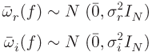
The likelihood detector derived under this System model V uses only the magnitude of the tag responses in the frequency domain. This tag detection technique is derived for an existing chipless RFID system that operates between 21 and 27 GHz. A circular resonator-based chipless RFID tags are designed and fabricated as described in Chapter 9. A printed tag encoded with bits ![]() is shown in Figure 10.5.
is shown in Figure 10.5.
Figure 10.5 A chipless tag coded with bits  .
.
Two tag prototypes were experimented to validate the theory. Tag type I is a retransmission tag operating over the frequency band of 2.2–2.6 GHz. The tag type II is a backscattering tag operating at 21–27 GHz. The experimental setup for validating tag type II is shown in Figure 10.6. In both experiments, the reader transmits a narrow-banded sinusoid signal using one horn antenna and the reader receives the tag response using a second antenna. The magnitude of the received signal is recorded along with the frequency of the signal sent. The frequency is swept across the 21–27 GHz band and the complete band response is recorded.
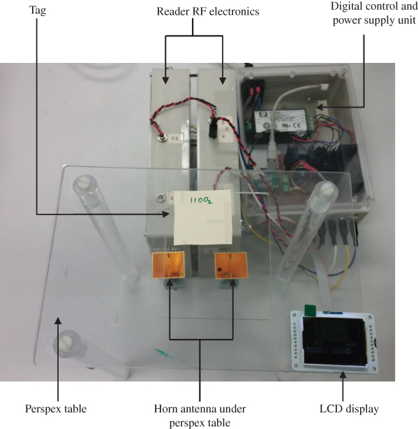
Figure 10.6 Experimental setup.
This process is repeated with all the possible 16 combinations for a 4-bit tag and the recorded tag responses are used with the tag detection technique derived for System model V to detect the encoded tag data bits.
In the following section, both simulation and experimental results are analyzed for the five tag detection techniques presented.
10.6 RESULTS
An interrogating signal is designed to provide a flat frequency response for at least 400 MHz around 2.4 GHz and it is used as the port excitation signal in CST simulations. Figure 10.7 shows the time- and frequency-domain interrogating signals. It can clearly be seen that the above requirement is achieved quite easily.
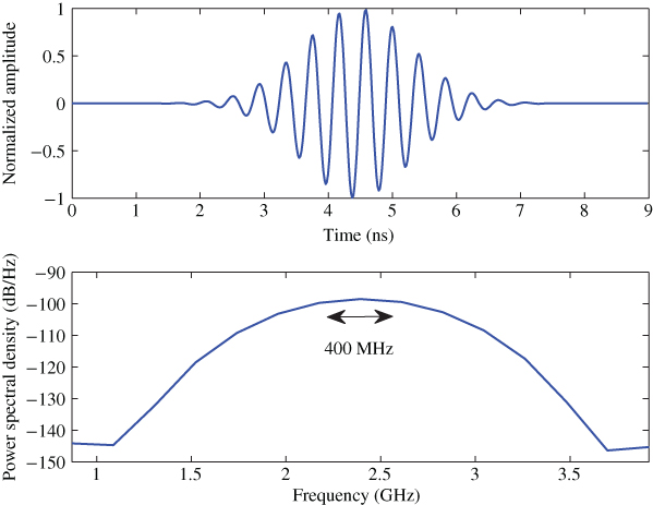
Figure 10.7 Interrogating signal in time and frequency domain.
Then the multiresonator tags are designed in CST according to the specifications given in Table 10.1. Initially, resonators are designed according to the frequency set 1 given in Table 10.1 that includes a guard-band between resonance frequencies. Then the resonators are redesigned in CST using the frequency set 2 without any guard-band. Then both time- and frequency-domain tag responses are obtained from CST simulations and stored in a lookup table for MATLAB simulations.
Figure 10.8 shows the frequency-domain response of a tag encoded with bits ![]() . It can clearly be observed that the resonances occur at the designed frequencies given by set 1 in Table 10.1. Figure 10.8 also shows the corresponding time-domain response of a tag encoded with bits
. It can clearly be observed that the resonances occur at the designed frequencies given by set 1 in Table 10.1. Figure 10.8 also shows the corresponding time-domain response of a tag encoded with bits ![]() .
.

Figure 10.8 Tag responses for  with a guard-band.
Then a new set of tag resonators are designed according to the frequency set 2 given in Table 10.1 without any guard-band. The frequency- and time-domain tag responses are illustrated in Figure 10.9. Similar to the previous simulation results, it can be concluded that the resonators are performing as expected by observing the resonance frequencies.

Figure 10.9 Tag responses for  without a guard-band.
Then these four resonators are arranged to implement the 16 tag combinations for a 4-bit tag. Simulations are repeated for 16 times and both time- and frequency-domain tag responses are obtained and recorded. Next the system models discussed in the previous section are implemented in MATLAB and the performances are analyzed. DERs under different SNR levels are calculated for each system model and the compared with a threshold-based tag detection system used in existing RFID readers. Simulation results for each system model are presented in the following sections.
10.6.1 System Model I
First, the DER is calculated at different noise power levels, effectively changing SIR and the result for System Model I is shown in Figure 10.10.

Figure 10.10 DER versus SNR for 4-bit tag with 60 MHz guard-band.
It can be seen that the DER is the same for both time- and frequency-domain-based samples. Therefore, it verifies the argument that the time-domain-based detection expression remains valid for the frequency-domain-based samples. When the frequency-domain-based samples are used, tag detection can be performed using the presence and absence of the power dips at resonating frequencies. This is achieved in existing chipless RFID readers using a threshold-based detection method that detects the power dips. This threshold-based detection method is used as the baseline comparison for the proposed tag detection methods.
As can be seen in 10.10, the proposed detection methods provide a significant improvement on DER over the threshold-based detection method. It can be seen that in order to achieve 99.99% reading accuracy, threshold-based detector needs an SNR of 19 dB. However, the proposed detector requires an SNR of only 11 dB, which is an SNR gain of 8 dB over the threshold-based detector. SNR can be related to the reading distance and SNR gain results in an increment in the tag reading range. The signal travels twice the distance between the reader and the tag. As a result, if the indoor propagation constant is assumed to be 2 [12], this SNR improvement can be related to improve the reader distance by a factor of 2.5. Therefore, the tag reading range can be improved by 2.5 times with the proposed tag detection technique while achieving a target reading accuracy of 99.99%.
On the other hand, this improved performance can be viewed as an increment in the tag reading accuracy at a given SNR. For example, the DER of the threshold-based detector at SNR = 10 dB is about 90%. With the proposed detector, the accuracy can be improved up to 99.95%. This avoids the requirement to perform multiple tag readings to detect one tag, especially under low-SNR scenarios. Therefore, depending on the application, improvement can be viewed on either the tag reading accuracy or the tag reading range.
Then the System Model I is used to detect the tag responses obtained using frequency set 2 given in Table 10.1. The removal of the guard-band causes the number of resonators allowed per unit bandwidth to be more than doubled in this example, which in turn double the tag bit capacity. As can be seen in Figure 10.11, traditional threshold-based decoder produces very poor performances when the guard-band is absent. For example, at an SNR of 10 dB the DER of the threshold-based method is about 60%. However, the proposed Signal Model I detector still achieves a high accuracy of 99% at the same SNR.

Figure 10.11 DER versus SNR without a guard-band between resonator frequencies.
Similar to the increment in the tag reading accuracy, the SNR gain of the proposed method compared to the baseline is also significant. For example, in order to achieve an accuracy of 90%, threshold-based detector requires at least an SNR of 19 dB while the proposed method requires only 3 dB providing an SNR gain of 16 dB, which is equivalent to a tag reading range improvement by six times. However, in reality the maximum reading range is limited by the mismatches in the tag orientation, antenna gain, transmitted power, and receiver's dynamic range. At large distances, all these factors contribute to cause performance deterioration.
For further clarity, Figure 10.12 shows a comparison of the DER for both threshold method and ML decoder under the presence and absence of a guard-band (GB). At lower SNR levels ( ![]() 5 dB) such as noisy industrial environment, the proposed detection method on both resonator sets performs similarly. However, at higher SNR levels, resonators with a guard-band perform better for obvious reasons. The key observation is that the threshold-based detector has very poor performances at compact tag resonators (without guard-band); however, the proposed detector still has an accepted level of tag reading accuracy. Therefore, it can be argued that the proposed detection method allows the tag data bit capacity to be doubled without compromising the tag reading performance. In addition, the likelihood expression is valid for both time- and frequency-domain-based sampling.
5 dB) such as noisy industrial environment, the proposed detection method on both resonator sets performs similarly. However, at higher SNR levels, resonators with a guard-band perform better for obvious reasons. The key observation is that the threshold-based detector has very poor performances at compact tag resonators (without guard-band); however, the proposed detector still has an accepted level of tag reading accuracy. Therefore, it can be argued that the proposed detection method allows the tag data bit capacity to be doubled without compromising the tag reading performance. In addition, the likelihood expression is valid for both time- and frequency-domain-based sampling.

Figure 10.12 DER versus SNR for ML decoder 1.
10.6.2 System Model II
After obtaining satisfactory performances from Model I, the System Model II is tested with both the real (I) and imaginary (Q) components of the received signal. Figure 10.13 shows the real and imaginary components of the baseband signal obtained after I/Q demodulation for tag response of [1111] when a 60 MHz guard-band is used between resonator frequencies.
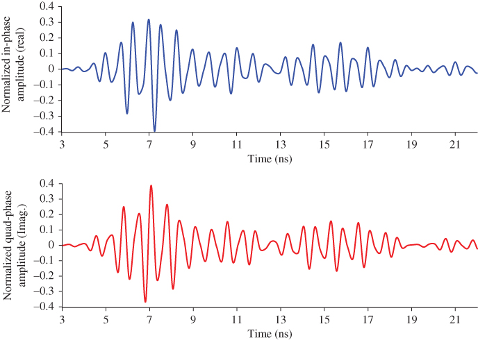
Figure 10.13 Real and imaginary samples of the tag response [1111].
FFT is performed on these I/Q samples and the tag response in frequency domain is obtained. Figure 10.14 illustrates the magnitude and phase of the frequency-domain tag response. It can clearly be seen that the information is encoded in both the magnitude and phase. As a result, it can be concluded that unlike in Model I, Model II uses the information used in both the I/Q samples. Therefore, it is expected to outperform the detector derived for Model I. These time- as well as the frequency-domain samples obtained by applying fast Fourier transformation to the time samples are used to calculate the DER at different SNR levels. Figure 10.15 shows a comparison of the DER for both the threshold method and ML decoder 2 when a guard-band is presented. It can be seen that the threshold detector achieves a tag reading accuracy of 99.99% at an SNR of 17 dB. The same level of reading accuracy can be achieved at 6 dB using ML decoder 2. The ML detector provides an SNR gain of 11 dB at 99.99% accuracy level that can be related to the improvement of the reading range by a factor of 3.5.

Figure 10.14 Frequency signature of tag type [1111].

Figure 10.15 DER versus SNR for ML decoder 2 with the presence of a guard-band.
On the other hand, at an SNR of 8 dB, the ML detector achieves and reading accuracy of 99.999% while the threshold detector manages only 70%. In addition, the proposed ML detector 2 has a tag reading accuracy of 95% at as low as 0 dB SNR. Therefore, it can also be concluded that the proposed ML detector 2 is performing well under low SNR levels. It is interesting to notice that ML detector 2 has an SNR gain of 3 dB compared to ML detector 1. This is due to the fact that ML detector 2 uses in information available in both the real and imaginary components of the received signal, whereas ML detector uses only the real component of the signal. A detailed comparison of the results obtained in different models is presented later in this section.
Figure 10.16 shows a comparison of the DER for both threshold method and ML decoder 2 when a guard-band is removed. Similar to System Model I, the threshold-based detector performs very poorly when the guard-band is removed. At an SNR of 10 dB, threshold-based detector has a reading accuracy of 50% while ML detector 2 achieves well over 99.99% tag reading accuracy. On the other hand, it is obvious that ML detector 2 provides an enormous SNR improvement over the threshold detector. This significant improvement is mainly due to the fact that unlike threshold detector the likelihood expression derived in Equation (10.15) is the optimum decoder as it uses the information available in both the real and imaginary components of the signal. A comprehensive comparison of the performances of the proposed detection techniques is presented at the end of Section 10.6.
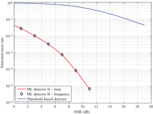
Figure 10.16 DER versus SNR for ML decoder 2 without a guard-band.
Figure 10.17 shows a comparison of the DER for both the threshold method and ML decoder 2 under the presence and absence of a guard-band. It is clear that for obvious reasons, both detectors perform well with the presence of a guard-band. However, once the guard-band is removed, threshold detector gets affected the most while ML decoder 2 still provides acceptable performances. ML detector performs well at lower noise levels regardless of the guard-band.

Figure 10.17 DER versus SNR for ML decoder 2.
In addition, it can be seen that even after removing the guard-band, Model II detector performs better than the existing threshold-based method. It can be interpreted as doubling the data capacity per unit bandwidth. In order to verify this claim, the simulations are repeated with eight resonators in the same bandwidth compared to four in the previous case. Figure 10.18 shows the calculated DER under 8 bits and compared against 4 bits tags with and without a guard-band. It can be seen that 4-bit tag with a guard-band has the best performance. Even though the 8-bit tag without a guard-band has the worst performance out of the three tags, it is comparable to that of the 4-bit tag without a guard-band. Hence, it is possible to conclude that the proposed detection algorithm doubles the tag data capacity.
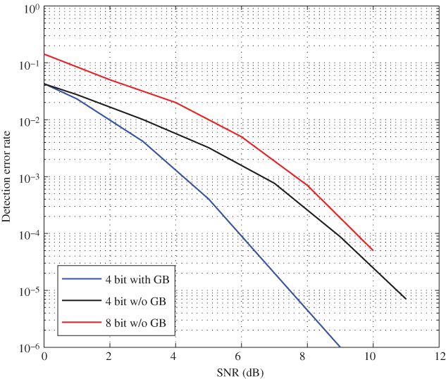
Figure 10.18 DER comparison for 8-bit tags.
10.6.3 System Model III
System Model III assumes an unknown channel with a known channel distribution. It is assumed that both the real and imaginary parts of the channel have the same Gaussian distribution due to symmetry. The mean and the standard deviation of the distribution are taken as 0.4 and 0.1, respectively. At different noise levels, DER is calculated based on both time and frequency samples and compared that with the baseline detection applied on frequency-domain samples.
Figure 10.19 shows a comparison of the DER for both threshold method and ML decoder 3 when a guard-band is presented. Unlike in previous two models, channel information is not available at the RFID reader. ML detector derived in this model uses the statistical properties of the channel for tag detection. Therefore, as expected, the performances are not very good as previous models, especially under low SNR scenarios. ML detector 3 achieves about 90% reading accuracy at SNR = 5 dB, which is still better than the 50% accuracy level of threshold-based detection. However, as SNR improves, the reading accuracy improves exponentially. For example, at an SNR of 10 dB, ML detector achieves an accuracy level of 99.95%, whereas threshold detector achieves only 90%.
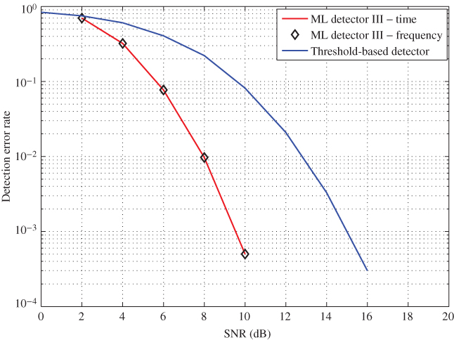
Figure 10.19 DER verus SNR for ML decoder 3 with the presence of a guard-band.
Moreover, ML detector achieves an accuracy level of 99.9% at SNR = 9 dB while threshold detector needs 15 dB in order to achieve the same accuracy level. This is an SNR gain of 6 dB, which is equivalent to the improvement of the reading range by a factor of 2. In addition, similar to previous models, time- and frequency-based ML detectors provide the same results.
Figure 10.20 shows a comparison of the DER for both the threshold method and ML decoder 3 when there is no guard-band presented. As expected, threshold-based detector has high DERs. For example, the reading accuracy of threshold detector at SNR = 10 dB is about 50%, while the proposed ML detector achieves an accuracy level of 99% at the same SNR. Even though the tag reading accuracy at lower SNR is poor, it improves exponentially as SNR increases. On the other hand, the proposed ML detector has an SNR gain of 10 dB over threshold detector when both detectors are expected to achieve an accuracy level of 95%. This SNR gain provides an improvement in reading range by a factor of 3. It can be concluded that the proposed ML-based detector performs better than the threshold-based detector used in existing RFID readers.

Figure 10.20 DER versus SNR for ML decoder 3 without a guard-band.
Figure 10.21 shows a comparison of the DER for both threshold method and ML decoder 2 under the presence and absence of a guard-band.

Figure 10.21 DER versus SNR for ML decoder 3.
It can clearly be seen that all of the detection methods failed to operate at lower SNR levels (![]() 5 dB). So it is safe to conclude that the assumptions to represent both the real and imaginary parts of the channel in a Gaussian distribution System Model III is valid only for higher SNR levels (
5 dB). So it is safe to conclude that the assumptions to represent both the real and imaginary parts of the channel in a Gaussian distribution System Model III is valid only for higher SNR levels (![]() 5 dB). However, ML-based detection technique performs better as the SNR improves regardless of the guard-band. The guard-band provides on average an SNR improvement of 2 dB for obvious reasons. Finally, it can be concluded that the proposed ML detection method allows to double the bit capacity of the chipless RFID tags without compromising the reading accuracy.
5 dB). However, ML-based detection technique performs better as the SNR improves regardless of the guard-band. The guard-band provides on average an SNR improvement of 2 dB for obvious reasons. Finally, it can be concluded that the proposed ML detection method allows to double the bit capacity of the chipless RFID tags without compromising the reading accuracy.
10.6.4 System Model IV
As described earlier, no channel information is available at the reader in System Model IV. This ML-based decoder detects both the tag type and the channel simultaneously. Similar to the previous cases, DER is calculated based on both time and frequency samples and compared that with the baseline detection applied on frequency-domain samples.
Figure 10.22 shows a comparison of the DER for both threshold method and ML decoder 3 when a guard-band is presented. Unlike the System Model III, this model performs better even at lower SNR levels. In this model, no assumptions are made to represent the channel. Instead, channel values are estimated along with the tag detection. It can be seen that, with the presence of a guard-band, ML detector achieves a reading accuracy level of 99.9% at SNR = 5 dB. However, threshold detector provides only 50% accuracy at the same SNR.
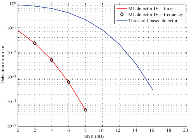
Figure 10.22 DER versus SNR for ML decoder 4 with the presence of a guard-band.
On the other hand, a reading accuracy of 99.9% is achieved by the proposed ML detector with an SNR gain of 10 dB over the threshold method. This results in improving the tag reading range by a factor of 3. In addition, both the time- and frequency-domain samples-based data provide the same performances as expected.
Figure 10.23 shows a comparison of the DER for both threshold method and ML decoder 3 when there is no guard-band presented. Following the trend in previous models, System Model IV performs well, even without a guard-band between resonance frequencies while the threshold detector has very poor performances. For example, at SNR =],5 dB, ML detector provides a reading accuracy of 99.5% while threshold detector provides on 20%. Apart from that, the proposed ML decoder provides an SNR gain of 17 dB over the threshold method when both are achieving a reading accuracy of 97%. This can be related to tag reading range being improved by a factor of 7. However, as explained earlier, this is possible only if the perfect tag orientation is achieved. The misorientation of the tag and the reader antennas may deteriorate the performance. After observing both aspects, it can be concluded that the proposed detection method allows to double the tag data bit capacity without compromising the tag reading performance.
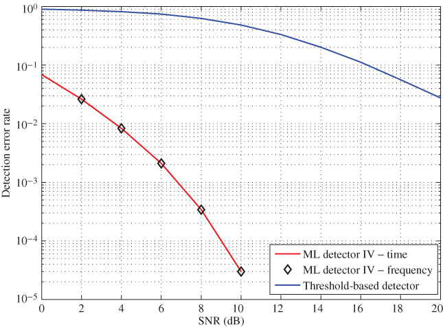
Figure 10.23 DER versus SNR for ML decoder 4 without a guard-band.
Figure 10.24 shows a comparison of the DER for both threshold method and ML decoder 2 under the presence and absence of a guard-band.

Figure 10.24 DER versus SNR for ML decoder 4.
A common feature of the results for System Model IV is that it performs well even under the lower SNR levels, regardless of the guard-band. As expected, at higher SNR levels, the guard-band provides an SNR gain of 2 dB. As mentioned at the beginning, ML detector 4 not only detects the tag but also estimates the channel.
10.6.4.1 Channel Estimation
The channel estimation accuracy is analyzed next. In MATLAB, a random channel is generated and used for system simulation. Then ML decoder 4 is used to calculate an estimate of the channel and compared with the actual channel. Figure 10.25 compares the estimated channel values obtained under number of iterations with the actual channel realization when a guard-band is presented between resonators in the chipless tag. It can be seen that the complex channel estimations are centered around the actual channel realization and the accuracy level of the estimations are very high at SNR = 14 dB. However, it does not demonstrate a clear picture of the distribution of the channel estimate.
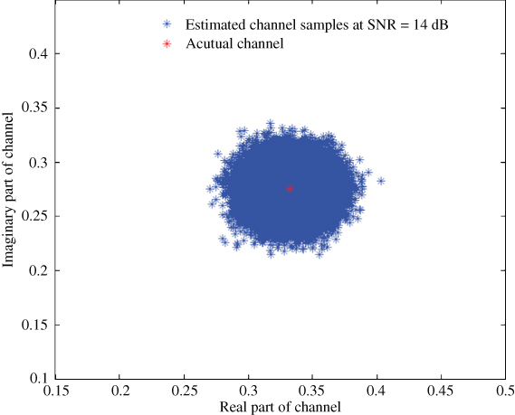
Figure 10.25 Channel estimation samples when a guard-band is presented.
Figure 10.26 shows the probability distribution function (pdf) of the channel estimation for both real and imaginary components. It compares the estimated channel with the actual channel realization, which is given by white-colored asterisks (*).

Figure 10.26 PDF of channel estimation when a guard-band is presented.
It can be clearly seen that the mean of each distribution is the same as the actual channel realization. In addition, both distributions have very similar but low variances. Therefore, it can be concluded that the proposed ML detection method estimates the channel accurately when a guard-band is presented.
Figure 10.27 compares the estimated channel values with the actual channel realization when more tag bits are presented leaving no guard-band between resonator frequencies in the chipless tag. The results show channel estimates obtained after a number of iterations at SNR = 10 dB. It is clear that even when the guard-band is not present, the proposed ML detector manages to estimate the channel accurately. The pdf of the estimates are calculated to closely observe the performance of channel estimation.

Figure 10.27 Channel estimation samples without a guard-band.
Figure 10.28 compares pdf of the channel estimation at SNR = 10 dB. Similar to the case with the guard-band, the mean of the distributions for both the real and imaginary components of the channel are approximately same as the actual channel realization. Moreover, the variances of both the real and imaginary components of the channel are very similar and low. The main difference between the cases having a guard-band and without is that the latter has a high variance compared to the former. It can be justified as the guard-band prevents interresonator interference causing less errors in the outcome of the ML detector used with tag responses having a guard-band.

Figure 10.28 PDF of channel estimation without a guard-band.
10.6.4.2 Comparative Study
Finally, DER performances of all the detection techniques described are compared and discussed. Figure 10.29 compares the DER performances of all the detection when a guard-band is presented between the tag resonance frequencies. It can be seen that ML detector 2 has the best performance out of all the detectors presented. ML detector 2 assumes perfect channel knowledge is available at the reader and uses information available in both real and imaginary components of the signal. This is the optimum detector for the chipless RFID system and hence can be treated as the upper margin for tag reading accuracy performances. The next best detector is ML detector 4, where the channel is completely unknown to the reader. ML detector 4 is a powerful detector as it not only achieves a higher tag reading accuracy but also estimates the channel with a high accuracy. ML detector 1 is the next best performer, where it assumes perfect channel knowledge and uses only the information available in the real part. This decoder does not exist in reality as this is derived first as the fundamental decoder and every other decoder is an extension of it.
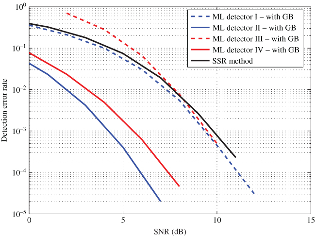
Figure 10.29 DER comparison with a guard-band.
Signal space representation (SSR) method used in Ref. [13] has similar performances to ML detector 1. This can be explained as both detectors use the information encoded in only on the magnitude. However, only five most dominant basis functions are used for SSR and leaving out the rest causes the performances to be slightly degraded. It can be concluded that SSR method almost achieves its upper limit performances that are the performances of ML detector 1. Even though both SSR and the proposed ML-based detection techniques require the same number of computations, SSR has slightly lower computation complexity in each iteration. For example, ML detector 1 calculates the minimum distance using the total number of samples of the received signal while SSR does it using only five samples that are the coordinates in five-dimensional space.
Finally, ML detector 3 shows similar performances to ML detector 1 at higher SNR levels. Its performance at lower SNR is poor compared to other detection techniques. This pinpoints that the Gaussian distribution model used for each real and imaginary part of the channel is not very accurate at lower SNR levels.
Figure 10.30 compares the DER performances of all the detection techniques when there is no guard-band between the tag resonator frequencies. Similar to the case with a guard-band, ML detector 2 has the best performance. It is interesting to notice that ML detector 4 achieves almost the upper margin even though no channel information is available. SSR method for this scenario uses only the most significant seven base functions. It can be seen that with seven base functions, SSR method achieves its upper margin performances, which are the performances of ML detector 1. This confirms that the proposed detection methods perform better than the SSR method.
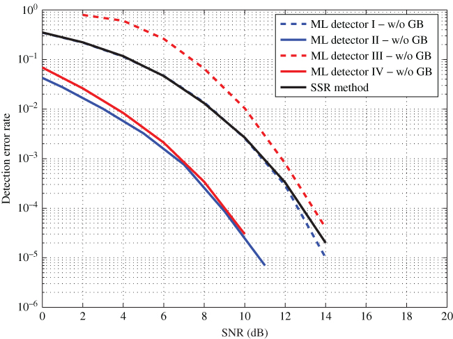
Figure 10.30 DER comparison without a guard-band.
However, at lower SNR levels (![]() 10 dB), ML detector 3 performs worse than ML detector 1. As the SNR increases (
10 dB), ML detector 3 performs worse than ML detector 1. As the SNR increases (![]() 10 dB), ML detector 3 performs similarly to ML detector 1. Similar to the case with a guard-band, even though System Model 3 models the system quite poorly at lower SNR levels, it is a valid detector for higher SNR levels. In addition, all ML-based detectors perform significantly better than the threshold-based detectors used in existing chipless RFID readers. Table 10.2 summarizes the results of all investigated methods so far.
10 dB), ML detector 3 performs similarly to ML detector 1. Similar to the case with a guard-band, even though System Model 3 models the system quite poorly at lower SNR levels, it is a valid detector for higher SNR levels. In addition, all ML-based detectors perform significantly better than the threshold-based detectors used in existing chipless RFID readers. Table 10.2 summarizes the results of all investigated methods so far.
Table 10.2 DER Comparison for Different Detection Methods
| SNR | 2 | 4 | 6 | 8 | 10 | 12 | |
| Threshold method | with GB | 7.0E−1 | 6.0E−1 | 4.0E−1 | 2.0E−1 | 8.0E−2 | 2.0E−2 |
| w/o GB | 9.0E−1 | 8.0E−1 | 7.0E−1 | 6.0E−1 | 5.0E−1 | 3.0E−1 | |
| SSR method | with GB | 2.5E−1 | 1.0E−1 | 4.0E−2 | 6.0E−3 | 8.0E−4 | N/A |
| w/o GB | 2.2E−1 | 1.2E−1 | 4.6E−2 | 1.3E−2 | 2.7E−3 | 3.3E−4 | |
| Model I | with GB | 2.1E−1 | 1.0E−1 | 3.1E−2 | 5.5E−3 | 4.5E−4 | 3.0E−5 |
| w/o GB | 2.2E−1 | 1.1E−1 | 4.7E−2 | 1.4E−2 | 2.6E−3 | 2.9E−4 | |
| Model II | with GB | 1.0E−2 | 1.0E−3 | 1.0E−4 | 3.0E−6 | N/A | N/A |
| w/o GB | 2.0E−2 | 6.0E−3 | 2.0E−3 | 3.0E−4 | 2.0E−5 | N/A | |
| Model III | with GB | 7.0E−1 | 2.8E−1 | 6.6E−2 | 7.7E−3 | 5.0E−4 | N/A |
| w/o GB | 8.0E−1 | 6.1E−1 | 2.6E−1 | 6.6E−2 | 1.0E−2 | 8.0E−4 | |
| Model IV | with GB | 2.3E−2 | 4.9E−3 | 6.2E−4 | 4.6E−5 | N/A | N/A |
| w/o GB | 2.6E−2 | 8.4E−3 | 2.1E−3 | 3.4E−4 | 3.0E−5 | N/A | |
10.6.5 System Model V
The likelihood detector derived under this model uses only the magnitude of the tag responses in the frequency domain. This tag detection technique is derived for an existing chipless RFID system that operates between 21 and 27 GHz. Figure 10.31 shows the tag response recorded by the chipless RFID reader.

Figure 10.31 Magnitude of the tag response for tag [1111].
The tag response received in Figure 10.31 together with all possible 16 combinations are used for the detection algorithm derived for System model V. Table 10.3 shows the likelihood values obtained for each tag type. In order to avoid underflow, probabilities are calculated in log to the base 10.
Table 10.3 Likelihood for each tag type
| Tag Type | Likelihood in Log Scale | Tag Type | Likelihood in Log Scale |
| [0000] | −35.41 | [1000] | −28.54 |
| [0001] | −28.50 | [1001] | −19.77 |
| [0010] | −27.76 | [1010] | −20.70 |
| [0011] | −22.87 | [1011] | −15.59 |
| [0100] | −29.76 | [1100] | −24.22 |
| [0101] | −22.47 | [1101] | −16.87 |
| [0110] | −22.28 | [1110] | −15.58 |
| [0111] | −17.31 | [1111] | −11.06 |
It can be clearly seen from Table 10.3 that tag type [1111] has the highest likelihood out of the 16 combinations. Therefore, the proposed detection technique has managed to detect the tag bits successfully.
A comprehensive analysis is performed using MATLAB simulations and Figure 10.32 shows both the simulated and experimental DER variation at different SNR levels. In addition, the results are compared with the threshold-based detection technique. It can be seen that the proposed tag detection technique has superior reading accuracy compared with the existing threshold-based detection technique. It is also important to notice that the experimental results agree with the simulated results. The experimental data is gathered only for two SNR levels as achieving low DERs at higher SNR levels are practically not feasible.

Figure 10.32 DER versus SNR for likelihood-based detector 5 for 21–27 GHz backscattering tag.
It can be concluded that the proposed tag detection technique for the magnitude-based chipless RFID reader achieves higher reading accuracy over the existing tag detection technique.
10.7 CONCLUSION
DER of a number of likelihood-based detectors were presented and compared against the threshold-based detector used in existing chipless RFID systems and the SSR method proposed in Ref. [13]. It is evident that all the likelihood-based detectors perform better than the threshold-based detector. ML detector 4 that jointly detects both the channel and the tag type achieves almost the optimum performance (ML detector 2). The improved performance of the proposed tag detection techniques directly relates to an increased tag reading accuracy at a given SNR level. On the other hand, it can also be represented as an increment in the reading range while achieving a particular goal of reading accuracy. Therefore, the improved performance can be represented either as increased reading accuracy or the reading range depending on the application.
However, there is a common drawback of all the likelihood-based detection methods discussed so far. All these methods require higher computation complexity compared to the primitive detection techniques such as threshold-based detection. For example, detecting a tag having ![]() bits involves evaluating the likelihood expressions for
bits involves evaluating the likelihood expressions for ![]() number of occasions. Two computationally feasible tag detection techniques have been introduced in Chapter 11 that can reduce the computation complexity from exponential to linear order without compromising on the chipless RFID tag reading accuracy.
number of occasions. Two computationally feasible tag detection techniques have been introduced in Chapter 11 that can reduce the computation complexity from exponential to linear order without compromising on the chipless RFID tag reading accuracy.
REFERENCES
- 1. S. Preradovic, I. Balbin, N. Karmakar, and G. Swiegers, “Multiresonator-based chipless RFID system for low-cost item tracking,” IEEE Transactions on Microwave Theory and Techniques, vol. 57, no. 5, pp. 1411–1419, May 2009.
- 2. S. Harma, V. Plessky, C. Hartmann, and W. Steichen, “PS-1 SAW RFID tag with reduced size,” in Ultrasonics Symposium, 2006. IEEE, Vancouver, BC, Canada, Oct 2006, pp. 2389–2392.
- 3. Y.-Y. Chen, T.-T. Wu, and K.-T. Chang, “P5H-3 A COM analysis of SAW tags operating at harmonic frequencies,” in Ultrasonics Symposium, 2007. IEEE, New York, NY, USA, Oct 2007, pp. 2347–2350.
- 4. S. Harma, V. Plessky, X. Li, and P. Hartogh, “Feasibility of ultra-wideband SAW RFID tags meeting FCC rules,” IEEE Transactions on Ultrasonics, Ferroelectrics, and Frequency Control, vol. 56, no. 4, pp. 812–820, April 2009.
- 5. S. Preradovic and N. Karmakar, “Design of fully printable planar chipless RFID transponder with 35-bit data capacity,” in Microwave Conference, 2009. EuMC 2009. European, Rome, Italy, Sept 2009, pp. 013–016.
- 6. IDTechEx, Chip-less RFID? The end game, 2006 (accessed December 24, 2014). [Online]. Available: http://www.idtechex.com/products/en/articles/00000435.asp.
- 7. K. C. Jones, Invisible tattoo ink for chipless RFID safe, company says, 2007 (accessed December 24, 2014). [Online]. Available: http://www.electronics-eetimes.com/en/invisible-tattoo-ink-for-chipless-rfid-safe-company-says.html?cmp_id=7& news_id=196900063.
- 8. S. Innovations, RFID Tattoo: Somark of the Beast, 2008 (accessed December 24, 2014). [Online]. Available: http://www.rap-con.com/signs/rfid-tattoo-somark-beast.
- 9. I. Jalaly and I. Robertson, “RF barcodes using multiple frequency bands,” in Microwave Symposium Digest, 2005 IEEE MTT-S International, Long Beach, CA, USA, June 2005, pp. 139–142.
- 10. J. McVay, A. Hoorfar, and N. Engheta, “Space-filling curve RFID tags,” in Radio and Wireless Symposium, 2006 IEEE, San Diego, CA, USA, Jan 2006, pp. 199–202.
- 11. S. Preradovic, I. Balbin, S. M. Roy, N. C. Karmakar, and G. Swiegers, “Radio frequency transponder,” Australian Provisional Patent Application P30 228AUPI, April, 2008.
- 12. G. Janssen and R. Prasad, “Propagation measurements in an indoor radio environment at 2.4 GHz, 4.75 GHz and 11.5 GHz,” in Vehicular Technology Conference, 1992, IEEE 42nd, May 1992, pp. 617–620 vol. 2.
- 13. P. Kalansuriya, N. Karmakar, and E. Viterbo, “Signal space representation of chipless RFID tag frequency signatures,” in Global Telecommunications Conference (GLOBECOM 2011), 2011 IEEE, Houston, TX, USA, Dec 2011, pp. 1–5.