
7 Column Stores
A row store is a row-oriented relational database as it was reviewed in Section 2.1. That is, data are stored in tables and on disk the data in a row are stored consecutively. This row-wise storage is currently used in most RDBMSs. In contrast, a column store is a column-oriented relational database. That is, data are stored in tables but on disk data in a column are stored consecutively.
This chapter discusses column stores and shows that they work very well for certain queries – for example queries that can be executed on compressed data. In such cases, column stores have the advantage of both a compact storage as well as efficient query execution. Conversion of nested records into columnar representation is a further topic of this chapter.
7.1 Column-Wise Storage
Column stores have been around and used since the 1970s but they had less (commercial) success than row stores. We take up our tiny library example to illustrate the differences:
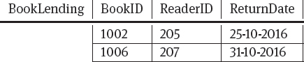
The storage order in a row store would be:
1002,205,25–10–2016,1006,207,31–10–2016
Whereas the storage order in column store would be:
1002,1006,205,207,25–10–2016,31–10–2016
Due to their tabular relational storage, SQL is understood by all column stores as their common standardized query language. For some applications or query workloads, column stores score better than row stores; while for others the opposite is the case. Advantages of column stores are for example:
Buffer management: Only columns (attributes) that are needed are read from disk into main memory, because a single memory page ideally contains all values of a column; in contrast, in a row store, a memory page might contain also other attributes than the ones needed and hence data is fetched unnecessarily.
Homogeneity:Values in a column have the same type (that is, the values come from the same attribute domain). This is why they can be compressed better when stored consecutively; this will be detailed in the following section. In contrast, in a row store, values from different attribute domains are mixed in a row (“tuple”) and hence a cannot be compressed well.
Data locality:Iterating or aggregating over values in a column can be done quickly, because they are stored consecutively. For example, summing up all values in a column, finding the average or maximum of a column can be done efficiently because of better locality of these data in a column store. In contrast, in a row store, when iterating over a column, the values have to be read and picked out from different tuples.
Column insertion:Adding new columns to a table is easy because they just can be appended to the existing ones. In contrast, in a row store, storage reorganization it necessary to append a new column value to each tuple.
Disadvantages of column stores lie in the following areas:
Tuple reconstruction:Combining values from several columns is costly because “tuple reconstruction” has to be performed: the column store has to identify which values in the columns belong to the same tuple. In contrast, in a row store, tuple reconstruction is not necessary because values of a tuple are stored consecutively. Tuple insertion:Inserting a new tuple is costly: new values have to be added to all columns of the table. In contrast, in a row store, the new tuple is appended to the existing ones and the new values are stored consecutively.
7.1.1 Column Compression
Values in a column range over the same attribute domain; that is, the have the same data type. On top of that columns may contain lots of repetitions of individual values or sequences of values. These are two reasons why compression can be more effective on columns (than on rows). Hence, storage space needed in a column store may be less than storage space needed in a row store with the same data. We survey five options for simple yet effective data compression (so-called encodings) for columns.
Run-length encoding:The run-length of a value denotes how many repetitions of the value are stored consecutively. Instead of storing many consecutive repetitions of a value we can store the value together with its starting row and its run-length (that is, the number of repetitions). That is, if in our table rows 5 to 8 would have the value 300 we have 4 consecutive repetitions and hence write (300,5,4) because this run of value 207 starts in row 5 and has a length of 4. This encoding is most efficient for long runs of repetitive values. As an example, let us have a look at the column ReaderID (see Table 7.1.); as readers can have several books at the same time, consecutive repetitions of the same reader ID are possible. In this case, when using the run-length encoding, we get a smaller representation of the same information.

Bit-vector encoding:For each value in the column we create a bit vector with one bit for each row. In each such bit vector for a given value, if the bit for the row is 1, then the column contains this value; otherwise it does not. Table 7.2. shows an example for the ReaderID column. This encoding is most efficient for relatively few distinct values and hence relatively few bit vectors.
Table 7.2.Bit-vector encoding

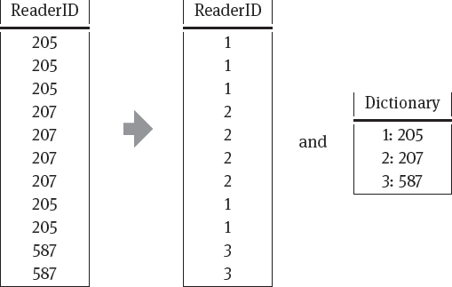
Table 7.4.Dictionary encoding for sequences

Dictionary encoding:We replace long values by shorter placeholders and maintain a dictionary to map the placeholders back to the original values. Table 7.3. shows an example for the ReaderID column.
In some cases, we could not only create a dictionary for single values but even for frequent sequences of values. As an example on the BookID column, assume that several sets of books are usually read together: books with IDs 1002, 1010 and 1004 would often occur together as well as books with IDs 1008 and 1006 would often occur together. Then our dictionary could group these IDs together and they can be replaced by a single placeholder (see Table 7.4.).
Frame of reference encoding:For the range of values stored in a column, one value that lies in the middle of this range is chosen as the reference value. For all other values we only store the off-set from the reference value; this offset should be smaller than the original value. Usually a fixed size of some bits is chosen for the offset. Table 7.5. shows an example for ReturnDate column.
Table 7.5.Frame of reference encoding

Table 7.6.Frame of reference encoding with exception

In case the offset for a value exceeds the fixed offset size, the original value has to be stored as an exception; to distinguish these exceptions from this offset a special marker (like #) is used followed by the original value. For example (see Table 7.6.), the offset between 25–10–2016 and 14–10–2016 might be too large, and we have to store 14–10–2016 as an exception when it is inserted into the column.
This encoding is only applicable to numerical data; it is most efficient for values with a small variance around the chosen reference value.
Table 7.7.Differential encoding

Table 7.8.Differential encoding with exception

Differential encoding:Similar to the frame of reference encoding, an offset is stored instead of the entire value. This time the offset is the difference between the value itself and the value in the preceding row. Table 7.7. shows an example for the ReturnDate column.
Again the offset should not exceed a fixed size. As soon as the offset gets too large, the current value is stored as an exception. In our example (see Table 7.8.), this is again the case when inserting the date 14–10–2016.
This encoding is only applicable to numerical data; it works best if (at least some) data are stored in a sorted way – that is, in decreasing or increasing order.
Note that with each encoding we have to maintain the order inside the column as otherwise tuple reconstruction would be impossible; that is, after encoding a column we cannot merge entries nor can we swap the order of the entries.
All these encodings cater for a more compact storage of the data. The price to be paid, however, is the extra runtime needed to compute the encoding as well as the runtime needed to decode the data whenever we want to execute a query on them. Fortunately, this decoding step might be avoided for certain classes of queries; that is, some queries can actually be executed on the compressed data so that no decompression step is needed. Let us illustrate such a case with the following example from our library database:

Now assume that the ReaderID is compressed with run-length encoding. That is, the column ReaderID is stored as a sequence as follows:
((205, 1, 3), (207, 4, 2), (205, 6, 1)).
An example query that can be answered on the compressed format is: “How many books does each reader have?”. Which would be in SQL:
SELECT ReaderID, COUNT(*) FROM BookLending GROUP BY ReaderID
To answer this, the column store does not have to decompress the column into the entire original column with 6 rows. Instead it just returns (the sum of) the run-lengths for each ReaderID value. Hence, the result for reader 205 is 3+1=4 and the result for reader 207 is 2:
Result: { (205, 4), (207, 2) }
7.1.2 Null Suppression
Sparse columns are columns that contain many NULL values, that is, many concrete values are missing. A more compact format of a sparse column can be achieved by not storing (that is, “suppressing”) these null values. Yet, some additional information is needed to distinguish the non-null columns from the null columns. We survey the options analyzed in [Aba07].
Position list:This is a list that stores only the non-null positions (the number of the row and its value) but discards any null values. As metadata the total number of rows and the number of non-null positions are stored. See Table 7.9. for an example.
Table 7.9.Position list encoding
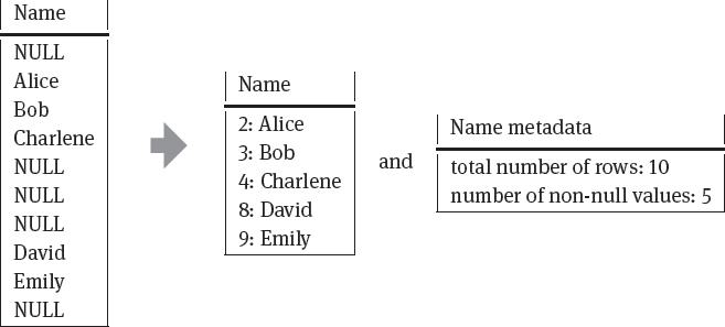
Table 7.10.Position bit-string encoding

Position bit-string:This is a bit-string for the column where non-null positions are set to 1 but null positions are set to 0. The bit-string is accompanied by a list of the non-null values in the order of their appearance in the column. See Table 7.10. for an example.
Position range:If there are sequences of non-null values in a column, the range of this sequence can be stored together with the list of values in the sequence. As metadata the total number of rows and the number of non-null positions are stored. See Table 7.11. for an example.
These three encodings suppress nulls and hence reduce the size of the data set. However, internally, query evaluation in the column store must be adapted to the null suppression technique applied.
7.2 Column striping
Google’s Dremel system [MGL+10] allows interoperability of different data stores. As a common data format for the different stores it uses a columnar representation of nested data. A schema for a nested record is defined as follows. A data element fi can either be of an atomic type or it can be a nested record. An atomic type can for example be an integer, a floating-point number, or a string; the set of all atomic values is called the domain dom. A nested record consists of multiple fields where each field has a name Ai as well as a value that is again a data element τ (that is, it it can have an atomic type or be another nested tuple). Fields can have multiplicities meaning that a field can be optional (written as ? and denoting that there can be 0 or 1 occurrences of this field) or that it can be repeated (written as * and denoting that there can be 0 or more occurrences of this field). Otherwise the field is required (that is, the field has to occur exactly once). Nesting is expressed by defining one field to consist of a group of subfields. Hence a data record τ can be recursively defined as
τ= dom| 〈A1 : τ[* |?], . . . , An : τ[* |?]〉
As an example, we consider several data records describing hotels. Each hotel has a required ID, as well as required hotel information (a group of subelements) consisting of a required name as well as a group of subelements for the address (containing a city) and a group of subelements for the roomprice (consisting of a price for a single room and a price for a double room). While the address group is optional the city is required; that is, whenever there is an address element it must contain a city element. The optional room price group for a hotel comprises an optional price for a single room as well as an optional price for a double room. Lastly, information on several staff members can occur repeatedly and each staff description contains a language item that can be repeated. Each hotel is represented in a document by a nested data record that complies with the following schema:
Table 7.11.Position range encoding

required string hotelID;
required group hotel {
required string name;
optional group address {
required string city;
}
optional group roomprice {
optional integer single;
optional integer double;
}
}
repeated group staff {
repeated string language;
}
}
Note that each such document (complying with the above schema) has a tree-shaped structure where only the leaf nodes carry values. The process of column striping decomposes a document into a set of columns: one column for each unique path (from the root to a leaf) in the document. For the example data record, column striping would result in one column for hotelID, one column for hotel.name, one column for hotel.address.city, one column for hotel.roomprice.single, one column for hotel.roomprice.double, and one column for staff.language.
For each unique path, the values coming from different documents (in the example, different hotel documents) are written to the same column in order to be able to answer analytical and aggregation queries over all documents efficiently. However we need some metadata to recombine an entire document as well as to be able to query it (and return the relevant parts of each document). These metadata are called the repetition level(to handle repetitions of paths) and the definition level(to handle non-existent paths of optional or repeated fields).
|
The repetition level for a path denotes at which level in the path the last repetition occurred. Only repeated fields in the path are counted for the repetition level. |
The repetition level can range from 0 to the length of the path: 0 means that no repetition has occurred so far, whereas the path length denotes that the entire path occurred for the previous field and is now repeated with the current field.
|
The definition level for a path denotes the maximum level in the path for which a value exist. Only non-required fields are counted for the definition level. |
To save storage space, only levels of non-required (that is, optional and repeated) fields are counted for the definition level; that is, required fields are ignored. The definition level can range from 0 to the level of the last optional or repeated field of the path. Some extra null values have to be inserted in case no value for the entire path but only for a prefix of the path exists. We derive the repetition and definition labels for an example.
For the example data record, we store six columns. For these six columns the potential definition and repetition levels can be obtained as follows:
–hotelID: Both the repetition and the definition level are 0 because the field is required.
–hotel.name: Both the repetition and the definition level are 0 because all fields in the path are required.
–hotel.address.city: The repetition level is 0 because no repeated fields are in the path. If the city field is undefined (that is, null), the address field must also be null (because otherwise the required city field would be defined); hence, the definition level will be 0 because the optional address field is not present. If in contrast the city field is defined, then the definition level is 1 because the optional address field is present.
–hotel.roomprice.single: The repetition level is 0 because no repeated fields are in the path. If the roomprice field is not present, the definition level is 0; if the roomprice field is present, but the single field is undefined, then the definition level is 1; in the third case, the single field is defined and hence also the roomprice field is present such that the definition level is 2.
–hotel.roomprice.double: The repetition level is 0 because no repeated fields are in the path. Similar to the above path, if the roomprice field is not present, the definition level is 0; if the roomprice field is present, but the double field is undefined, then the definition level is 1; in the third case, the double field is defined and hence also the roomprice field is present such that the definition level is 2.
–staff.language: Because the two fields in the path are repeated, both the repetition level as well as the definition level are incremented, depending on whether the fields are defined and considering the preceding path in the same document to count the repetitions.
–If the staff element is not present at all, then the repetition level and the defi-nition level are both 0.
–If the current path only contains a staff field (without any language field), then the definition level is 1; the repetition level depends on the preceding path in the same document: if in the preceding path a staff field is present, then the repetition level is 1 otherwise it is 0.
–If the current path contains a language field (inside a staff field), the definition level is 2. If the preceding path in the same document contains a staff field (without any language field), then the repetition level is 1; if preceding path in the same document contains a staff field and a language field, the current and the preceding language field can either be subfields of the same staff field (then the repetition level is 2) or the current and the preceding language field are subfields of two different staff fields (then the repetition level is 1); otherwise the repetition level is 0.
In the example, three different hotels are stored in the system each complying with the above definition of a data record. Note that the nesting of the staff.language element differs (in some cases the language element repeats at level 1 in other cases at level 2) and that some non-required fields (like roomprice and staff) are missing from some records.
hotelID : ‘h1’
hotel :
name : ‘Palace Hotel’
staff :
language : ‘English’
staff :
language : ‘German’
language : ‘English’
staff :
language : ‘Spanish’
language : ‘English’
hotelID : ‘h2’
hotel :
name : ‘Eden Hotel’
address :
city : ‘Oldtown’
roomprice :
single : 85
double : 120
hotelID : ‘h3’
hotel :
name : ‘Leonardo Hotel’
address :
city : ‘Oldtown’
roomprice :
single : 85
double : 120
hotelID : ‘h3’
hotel :
name : ‘Leonardo Hotel’
address :
roomprice :
double : 100
staff :
language : ‘English’
staff :
language : ‘French’
Each document can be sequentially written as a set of key-value pairs; the number of levels in each key depends on the level of nesting in the document. Our hotel documents can hence be written as the following sequence where null values are explicitly added for non-existent fields:
hotelID : ‘h1’,
hotel.name : ‘Palace Hotel’,
hotel.address : null,
hotel.roomprice.single : null,
hotel.roomprice.double : null,
staff.language : ‘English’,
staff.language : ‘German’,
staff.language : ‘English’,
staff.language : ‘Spanish’,
staff.language : ‘English’,
hotelID : ‘h2’,
hotel.name : ‘Eden Hotel’,
hotel.address.city : ‘Oldtown’,
hotel.roomprice.single : 85,
hotel.roomprice.double : 120,
staff.language : null,
hotelID : ‘h3’,
hotel.name : ‘Leonardo Hotel’,
hotel.address.city : ‘Newtown’,
hotel.roomprice.single : null,
hotel.roomprice.double : 100,
staff.language : ‘English’,
staff.language : ‘French’
The problem with this sequential representation is that the staff information is ambiguous: some staff members speak two languages (so that the language element at level 2 is repeated) while in other cases there are two staff members speaking one language each (so that the staff element at level 1 is repeated). To avoid this ambiguity, the repetition level for each field is added. Moreover definition levels are calculated to retain the structure information for non-existent fields.
hotelID : ‘h1’ (rep: 0, def: 0),
hotel.name : ‘Palace Hotel’ (rep: 0, def: 0),
hotel.address : null (rep: 0, def: 0),
hotel.roomprice.single : null (rep: 0, def: 0),
hotel.roomprice.double : null (rep: 0, def: 0),
staff.language : ‘English’ (rep: 0, def: 2),
staff.language : ‘German’ (rep: 1, def: 2),
staff.language : ‘English’ (rep: 2, def: 2),
staff.language : ‘Spanish’ (rep: 1, def: 2),
staff.language : ‘English’ (rep: 2, def: 2),
hotelID : ‘h2’ (rep: 0, def: 0),
hotel.name : ‘Eden Hotel’ (rep: 0, def: 0),
hotel.address.city : ‘Oldtown’ (rep: 0, def: 1),
hotel.roomprice.single : 85 (rep: 0, def: 2),
hotel.roomprice.double : 120 (rep: 0, def: 2),
staff.language : null (rep: 0, def: 0),
hotelID : ‘h3’ (rep: 0, def: 0),
hotel.name : ‘Leonardo Hotel’ (rep: 0, def: 0),
hotel.address.city : ‘Newtown’ (rep: 0, def: 1),
hotel.roomprice.single : null (rep: 0, def: 1),
hotel.roomprice.double : 100 (rep: 0, def: 2),
staff.language : ‘English’ (rep: 0, def: 2),
staff.language : ‘French’ (rep: 1, def: 2)
Finally all entries for each path are stored in a separate column table with the repetition and definition levels attached. See Table 7.12. for the final representation of our example.
To achieve a compact representation, for paths only containing required fields (where repetition and definition levels are always 0) the repetition and definition levels are not stored at all. A similar argument applies to the value null: it suffices to store the definition and repetition level and represent the value null as an empty table cell.
While the column striping representation allows for a compact and flexible storage of records, the query answering process needs to recombine the relevant data from the appropriate column tables; this process is called record assembly. In order to answer queries on the column-striped data records, finite state machines (FSM) are defined that assemble the fields in the correct order and at the appropriate nesting level. The advantage is that only fields affected by the query have to be read while other fields (in particular in other columns) are not accessed.
Table 7.12.Column striping example

For example, to assemble only the hotelID as well as staff.language data, only few transition rules are needed as shown in figure 7.1. We need rules that start the record with the hotelID and then jump to the staff.language element until the end of the record is reached.
These rules mean that current the row will be read and output with a nesting structure according to the definition level; after outputting the current row, we look at the repetition level of the next row and apply the transition rule for which the repetition level corresponds to the transition condition. For null values the definition levels are interpreted to determine which prefix of the path was part of the document.

Fig. 7.1.Finite state machine for record assembly
7.3 Implementations and Systems
In this section, we present a column store system and an open source implementation of the column striping algorithm.
7.3.1 MonetDB
MonetDB is a column store database with more than two decades of development experience.
|
Web resources: –MonetDB: https://www.monetdb.org/ –documentation page: https://www.monetdb.org/Documentation –Mercurial repository: http://dev.monetdb.org/hg/MonetDB/ |
It stores values in so-called binary association tables (BATs) that consist of a head and a tail column; the head column stores the “object identifier” of a value and the tail column stores the value itself. Internally, these columns are stored as memory-mapped files that rely on the fact that the object identifiers are monotonically increasing and dense numbers; values can then efficiently be looked up by their position in virtual memory. For query execution, MonetDB relies on a specialized algebra (BAT algebra) that processes in-memory arrays. Internally, these BAT algebra expressions are implemented by a sequence of low-level instructions in the MonetDB Assemblee Language (MAL). Several optimizers are part of MonetDB that make execution of MAL instructions fast.
7.3.2 Apache Parquet
Apache Parquet implements the column striping approach explained in Section 7.2.
|
Web resources: –Apache Parquet: http://parquet.apache.org/ –documentation page: http://parquet.apache.org/documentation/latest/ –GitHub repository: https://github.com/apache/parquet-mr |
For efficient handling the striped columns are divided into smaller chunks (column chunks). Column chunks consist of several pages (the unit of access) where each page stores definition levels, repetitions levels and the values. Moreover, several column chunks (column chunks coming from different striped columns) are grouped into row groups; that is, a row group contains one column chunk for each column of the original data and hence corresponds to a horizontal partitioning. Several row groups are stored in a Parquet file together with some indexing information and a footer. Among other information the footer stores offsets to the first data page of each column chunk and the indexes. These metadata are stored in a footer to allow for single-pass writing: the file is filled with row groups first and then the metadata is stored in the end. However, when reading the data, the metadata have to be accessed first. More precisely, in the footer there are file metadata (like version and schema information) as well as metadata for each column chunk in a page of the file. If the file metadata are corrupted, the file cannot be read. Additionally each page contains metadata in a header. Based on the metadata, those pages that are of no interest to the reader can be skipped. Parquet supports run-length encoding as well as dictionaries but can be extended by custom column compression or encoding schemes.
7.4 Bibliographic Notes
Column-oriented storage organization of relational data has been investigated since the 1970s and has been come to known as the decomposition storage model [LS71, CK85, KCJ+87]. Extending these foundational approaches, several column store systems are nowadays available. For example, the open source product MonetDB [IGN+12] calls itself “the column store pioneer” and fully relies on column-wise storage of data. Vectorwise [ZB12] offers several optimizations “beyond column stores”. The research project C-Store [SAB+05] has been continued as the Vertica system [LFV+12]. Many other commercial systems use column store technology for fast analytical queries. The journal article [ABH+13] gives a profound overview of column store technology including compression, late materialization and join optimizations. Compression methods and their performance trade-offs are studied in several articles like [RH93, AMF06, HRSD07, KGT+10, Pla11]. In addition, [SFKP13] also present indexing on columns. Pros and cons of row stores versus column stores have been analyzed in different settings – for example, [HD08] or [AMH08].