4Graph Databases

A graph is a structure that not only can represent data but also connections between them; in particular, links between data items are explicitly represented in graphs. In this chapter, we first of all establish the necessary theoretic background on graphs and then shift to data structures that can be used to store graphs. Advanced graph structures allow for a representation of data of an even higher complexity.

4.1 Graphs and Graph Structures

Graphs structure data into a set of data objects (which may have certain properties and are equivalent to entities in the relational terminology) and a set of links between these objects (which characterize the relationship of the objects). The data objects are the nodes (also called vertices) of the graph and the links are the edges (also called arcs). Recall that one criticism towards the relational data model was its semantic overloading were entities and relationships are both represented as relational tables (see Section 3.1). We now see that for the graph data model the distinction between data objects (entities) and their relationships comes very naturally. Common applications for graph databases are hence domains where the links between data objects are important and need to have their own semantics.

Graphs can store information in the nodes as well as on the edges.

For example, in a social network the nodes of a graph can store information on people in the social network and edges can store their acquaintance or express sympathy or antipathy (see Figure 4.1). Another typical application are geographic information systems where nodes store information on geographical locations like cities and edges store for example the distances between the locations (see Figure 4.2).

4.1.1 A Glimpse on Graph Theory

From a mathematical point of view, a graph G consists of a set of vertices (denoted V) and a set of edges (denoted E); that is, G = (V, E). The edge set E is a set of pairs of nodes; that is, each edge is represented by those two vertices that are connected by the edge. An edge can be directed (with an arrow tip) or undirected. In case of a directed edge the pair of nodes is ordered where the first node is the source node of the edge and the last node is the target node; in the undirected case, order of the pair of nodes does not matter because the edge can be traversed in both directions. A graph is called undirected if it only has undirected edges, whereas a graph is called directed (or a digraph) if it only has directed edges. Moreover, a graph is called multigraph if it has a pair of nodes that is connected by more than one edge. Let us have a look at some examples.

Simple undirected graph: For a simple undirected graph (without multiedges and directed edges), each edge is represented by a set of vertices. That is, the edge set E is a set of two-element subsets of V (like {v1, v2}). Note that in the set notation order is irrelevant: that is, {v1, v2} and {v2, v1} are the same edge. For the cardinality of the vertex set |V| = n there are at most edges (without self-loops like {v1, v1}). Such a graph is called complete if E is the set of all two-element subsets of V. An example of a complete simple undirected graph with three vertices is the following:

–the vertex set is V = {v1, v2, v3}

–the edge set is E = {e1, e2, e3} = {{v1, v2}, {v2, v3}, {v1, v3}}

–the cardinality of the vertex set is |V| = 3, and hence we have edges in a complete graph

Simple directed graph: For a simple directed graph, each edge is represented by an ordered tuple of vertices like (v1, v2), where v1 is the source node and v2 is the target node. In this case, the order of the tuple denotes the direction of the edge: that is, (v1, v2) and (v2, v1) are distinct edges. More generally, the edge set E is a subset of the cartesian product V × V. For the cardinality of the vertex set |V| = n there are at most edges (without self-loops like (v1, v1)). The graph is called complete if E is the set of all tuples in V × V. The graph is called oriented if it has no symmetric pair of directed edges (no 2-cycles) – that is, there are no two edges where the source node of the first edge is the target node of the second edge and the other way round. An example of an oriented simple directed graph is the following:

–the vertex set is V = {v1, v2, v3}

–the edge set is E = {e1, e2, e3} = {(v1, v2), (v2, v3), (v1, v3)}

–this graph is not complete because 3! (3−2)! = 6 but there are only three edges – this graph is oriented because there are no backward edges

Undirected Multigraph: For an undirected multigraph, the edge set E is a multiset of two-element subsets of V. That is, duplicate elements are allowed and hence multiple edges between two vertices are possible; this set of vertices is then called multiedge. Sometimes, cardinalities are written on a multiedge instead of drawing the edge multiple times. An example of an undirected multigraph is the following:

–the vertex set is V = {v1, v2, v3}

–the edge set is E = {e1, e2, e3, e4} = {{v1, v2}, {v2, v3}, {v1, v3}, {v1, v3}} where e3 and e4 are duplicates

Directed Multigraph: For a directed multigraph, the edge set E is a multiset of tuples of the cartesian product V × V. Hence, multiple edges (with the same direction) between two vertices are possible. An example of a directed multigraph is the following:

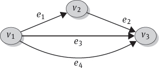
–the vertex set is V = {v1, v2, v3}

–the edge set is E = {e1, e2, e3, e4} = {(v1, v2), (v2, v3), (v1, v3), (v1, v3)} where e3 and e4 are duplicates.

Weighted graphs: With weighted graphs, each edge has a cost called weight and written as wi. This cost can for example denote the distances between cities as seen in Figure 4.2. An example of a weighted directed multigraph is the following:

–the vertex set is V = {v1, v2, v3}

–the set of edges with weights is E = {e1 : w1 , e2 : w2 , e3 : w3 , e4 : w4} = {(v1, v2) : w1 , (v2, v3) : w2 , (v1, v3) : w3 , (v1, v3) : w4}

As we will see later, the prevailing data structure used in graph databases is a directed multigraph (where information is stored in the nodes as well as on the edges).

4.1.2 Graph Traversal and Graph Problems

A connection between to nodes consisting of intermediary nodes and the edges between them is called a path; a path where starting node and end node are the same is called a cycle. The basic form of finding certain nodes in a graph is navigation in a graph by following some path; in graph terminology, this is called the traversal of a graph. More precisely, a traversal usual starts from a starting node (or a set of starting nodes) and then proceeds along some of the edges towards adjacent (that is, neighboring) nodes. A traversal may be full (that is, visiting each and every node in a graph) or it may be partial. For a partial traversal, navigation may be restricted by a certain depth of paths to be followed, or by only accessing nodes with certain properties.

The two simplest kinds of a full traversal are depth-first search and breadth-first search, which both depend on a certain order of the adjacent nodes: From the starting node, depth-first search follows the edge to the first adjacent node (in the given order) and then proceeds towards the first adjacent node of the same; breadth-first search visits all adjacent nodes of the starting node (in the given order) and then does the same with the adjacent nodes of its first adjacent node, then of its second adjacent node and so on. When traversing a graph, restrictions may be applied that have come to known as graph problems. For example for full traversals, graph problems are:

Eulerian Path: a path that visits each edge exactly once; that is, starting node and end node need not be identical, but each edge has to be traversed. In order to cover all edges, it might be necessary to visit some nodes more than once.

Eulerian Cycle: a cycle that visits each edge exactly once; that is, starting node and end node have to be the same and each edge has to be traversed.

Hamiltonian Path: a path that visits each vertex exactly once. In this case it might happen that not all edges have to be traversed.

Hamiltonian Cycle: a cycle that visits each vertex exactly once.

Spanning Tree: a subset of the edge set V that forms a tree (starting from a root node) and visits each node of the tree.

Problems for partial traversals also exist; a common example is finding the shortest path between two nodes. For weighted graphs, several variants of graph problems exist that aim at optimizing the weights; for example, finding a path between two nodes with minimal cost (where the cost is the sum of all weights on the path) or finding a spanning tree with minimal cost.

4.2 Graph Data Structures

When computing with graphs, the information on nodes and their connecting edges has to be represented and stored in an appropriate data structure. Two important terms in this field are adjacency and incidence. In directed graphs, one must further differentiate incidence with respect to incoming and outgoing edges: one node is the source node (for which the edge is an outgoing edge) while the other one is the target node of the edge (for which the edge is an incoming edge). Other terms for source node and target node are tail node and head node, respectively.

Two nodes are adjacent if they are neighbors (that is, there is an edge between them). An edge is incident to a node, if it is connected to the node; if the edge is directed, it is positively incident to its source node and negatively incident to its target node. A node is incident to an edge, if it is connected to the edge.

In general, for the representation of edges, we have the following choices where each representation has its own advantages and disadvantages.

4.2.1 Edge List

The graph can be stored according to the mathematical definition as a set of nodes V and a set (or list) of edges E. Depending on the type of graph the edge set will be implemented as a set of sets (for undirected graphs), a set of tuples (for directed graphs), as well as a normal set (for simple graphs) or a multiset (for multigraphs). As soon as a node is created it can simply be added to the node set V; when an edge is created, it is simply added to the edge set E. The same applies to deletions by simply deleting the removed node or edge from the respective set. The edge set performs well when one wants to retrieve all edges of the graph at once and it incurs no storage overhead (that is, it stores only existence of edges but not the absence of edges). However, the edge list representation is ineffcient in most use cases: for example, looking for one particular edge or getting all neighbors of a given node requires iterating over the entire edge list, which quickly becomes infeasible for larger edge sets.

4.2.2 Adjacency Matrix

For cardinality |V| = n the adjacency matrix is an n×n matrix where rows and columns denote all the vertices v1 . . . vn. For edgeless graphs the matrix contains only 0s; when edges exist in the graph some matrix cells are filled with 1s as follows.

For a simple undirected graph, if an edge {vi, vj} between vi and vj exists, write 1 into the matrix cell where vi is the row and vj is the column and another 1 where vi is the column and vj is the row; that is the matrix is symmetric. For the example graph, the adjacency matrix is:

Note that in practice a symmetric matrix would be stored as a triangular matrix by skipping all entries above the diagonal. For an undirected graph with loops, for a loop {vi, vi} write 2 into the appropriate matrix cell on the diagonal (because all edges are counted symmetrically).

For a simple directed graph, if an edge (vi, vj) from vi to vj exists, write 1 into the matrix cell where vi is the column and vj is the row; that is, the matrix is asymmetric. This is also the case for the example graph:

For a directed graph with loops, for a loop (vi, vi) write 1 into the appropriate matrix cell on the diagonal (because all edges are counted asymmetrically).

For an undirected multigraph, if k edges {vi, vj} between vi and vj exist, write k into the matrix cell where vi is the row and vj is the column and another k where vi is the column and vj is the row; again the matrix is symmetric because edges are undirected.

For an undirected multigraph with loops, for k loops {vi, vi} write 2 • k into the appropriate matrix cell on the diagonal (because all edges are counted symmetrically).

For a directed multigraph, for k edges (vi, vj) from vi to vj, write k into the matrix where vi is the column and vj is the row (again we have an asymmetric matrix).

For a directed multigraph with loops, for k loops (vi, vi) write k into the appropriate matrix cell on the diagonal (because all edges are counted asymmetrically).

The advantages of the adjacency matrix lie in a quick lookup of the existence of a single edge (given its source node and its target node) by simply looking up the bit value in the corresponding matrix cell as well as a quick insertion of a new edge (between two existing nodes) by just incrementing the bit in the matrix cell. The disadvantages are that adding a new node requires insertion of a new row and a new column and finding all neighbors results in a scan of the entire column. The main issue with this matrix representation is that it has a high storage overhead: due to its size |V| × |V| it soon gets very spacious for a larger number of nodes. This is due to the fact that it stores lots of unnecessary information – at least when there are lots of 0s (that is, the matrix and hence the graph are sparse). Thus, the matrix representation is usually only applicable for dense graphs; that is, for graphs where most of the edges are present.

4.2.3 Incidence Matrix

For cardinality |V| = n and |E| = m the incidence matrix is an n × m matrix where rows denote vertices v1 . . . vn; and columns denote edges e1 . . . em. For edgeless graphs the matrix contains no columns; as soon as edges are present, columns are created and filled as follows.

For a simple undirected graph if edge ei is connected (that is, incident) to vj, write 1 for column ei and row vj. For example:

For an undirected graph with loops, for a loop ei = {vj, vj} write 2 for column ei and row vj.

For a simple directed graph, the source node has to be distinguished from the target node of an edge. We use -1 for the source node (vi) and 1 for the target node (vj); that is, for an edge ek = (vi, vj), write -1 into the matrix for column ek and row vi, 1 for column ek and row vj. For example:

For a directed graph with loops, for a loop ek = (vi, vi) write 2 for column ek and row vi.

For an undirected multigraph the same procedure applies as for an undirected simple graph because each edge (even if being part of a multiedge) has its own edge identifier. For example:

For a directed multigraph the same procedure applies as for directed simple graph because each edge (even if being part of a multiedge) has its own edge identifier. For example:

One advantage of the incidence matrix is that only existing edges are stored; that is, there is no column with only 0 entries. The disadvantages of the incidence matrix are similar to the adjacency matrix. Insertions of new vertices and edges are costly because they require addition of a row or a column, respectively. Determining all neighbors for one vertex requires scanning the entire row and for each non-zero entry (1 in the undirected and -1 in the directed case) looking up where the other end point (that is, the other 1 entry) is located in the same column.

Note that checking the existence of an edge (for a given source node and target node) is more involved for the incidence matrix than for the adjacency matrix: we have to check whether there is a column with appropriate non-zero entries for the source node’s row and the target node’s row. In particular, the n×m matrix is storage intensive for a larger number of edges and vertices. And what makes incidence matrices even worse is the fact that if there are many vertices, there are lots of 0s in the columns because usually there will be only two non-zero entries in each column – as a side note it might however be mentioned that hyperedges (see Section 4.5) can be stored by having more than two non-zero entries in the edge’s column.

4.2.4 Adjacency List

With an adjacency list, one stores the vertex set V and for each vertex one stores a linked list of neighboring (that is, adjacent) vertices.

For a simple undirected graph, each edge is stored in the adjacency list of both its vertices; that is, one node on an edge is contained in the adjacency list of the other node. For example:

For a simple directed graph, the adjacency list stores only outgoing edges; that is, the adjacency list of one node is only filled when this node is a source node of some edge and it then contains only the target nodes of such edges. For example:

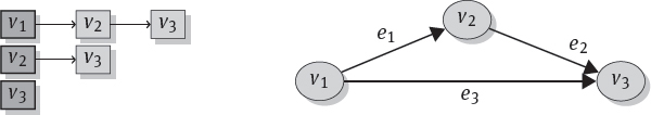
For multigraphs, in both the directed as well as the undirected case, nodes can occur multiple times in an adjacency list – depending on the amount of multiedges between the two nodes. For example:

With the adjacency list, we have the advantage of a flexible data structure, where new vertices can be quickly inserted (by just adding it to V) and, similarly, edges can be quickly inserted (by appending a node to the appropriate adjacency list). Furthermore, we have a quick lookup of all neighboring vertices of one vertex (by just returning its adjacency list) and no storage overhead occurs (because only relevant information is stored). However these advantages come at the cost of some disadvantages – in particular, with respect to the runtime behavior. For example, checking existence of a single edge (for a given source node and target node) requires a full scan of the adjacency list of the source node.

4.2.5 Incidence List

With the incidence list, each edge has its representation as an individual data object (instead of being only implicit as is the case with edges in the adjacency list); this allows for storing additional information on the edge in the edge object (in our example, the additional information is the name of the edge). More precisely, with an incidence list, you store the vertex set V and for each vertex you store a linked list of incident edges. When the edge is directed, the edge object contains information on its source node and its target node (like a tuple (vi, vj)) and the edge can only be traversed from source to target; in the undirected case no difference is made between source and target nodes: they are stored as a set (like the set {vi, vj}) and the edge can be traversed in both directions.

For a simple undirected graph, each undirected edge is contained in the incidence lists of its two connected nodes.

For a simple directed graph, it suffces to store only outgoing edges in the incidence list as long as only a forward traversal of the edges is needed. However, for some queries on graphs sometimes a backward traversal of an edge is necessary. An example for a backward traversal in a social network with directed edges would be: “Find all my friends who like me”. In this case, the “like”-edge has to be traversed from the target (“me”) towards the sources (the “friends”). In this case, it is advantageous to store all incident edges in a node’s incidence list to allow for both forward traversal of the outgoing edges and backward traversal of the incoming edges. Indeed, we could even have two incidence lists: one with outgoing edges for the forward traversal, and another one for incoming edges for the backward traversal.

In our example we only show the incidence lists for a forward traversal:

For multigraphs, in both the directed as well as the undirected case, each edge has its own identity (even when being part of a multiedge as is the case for e3 and e4) and hence is stored separately. For example, in the undirected case, each edge contains again pointers to the incident nodes:

In the directed case, each edge would have a pointer to its source node as well as one pointer to its target node:

In practical implementations, the incidence list would be stored inside a node object as a collection of pointers to incident edge objects – potentially – in the directed case – one collection for incoming and one collection for outgoing edges to allow for both forward and backward traversal. This means that – in contrast to the above illustrations – no duplicate edge objects (the ones with identical names) occur. Each edge object would in turn contain a collection of pointers to its incident nodes – in the undirected case; or alternatively – in the directed case – one pointer to the source node of the edge (“positive incidence”) and one to the target node (“negative incidence”).

Similar to the adjacency list, the incidence list is a flexible data structure for storing graphs. In addition, because incidence lists treat edges as individual data objects, information can be stored in an edge. This is important in most practical cases, for example with the property graph model discussed in the following section.

4.3 The Property Graph Model

When it comes to using graphs for data storage, the basic storage structure usually is a directed multigraph. However, some extensions to the mathematical graph definition are due: we must be able to store information inside the nodes as well as along the edges. More formally, the graph structures described in Section 4.1.1 consider only one kind of edge and one kind of node and are hence called single-relational graphs. However for most practical purposes, we must be able to distinguish different kinds of nodes (for example, Person nodes or City nodes) as well as different kinds of edges. This is achieved by so-called multi-relational graphs where types are introduced for nodes and for edges. A type first of all has a name like “Person” for a node type or “likes” for an edge type. Each node is labeled with the name of a node type and each edge is labeled with the name of an edge type; that is, the node label denotes the corresponding node type, and the edge label denotes the edge type. Apart from the name, a type defines attributes for the corresponding nodes and edges. More precisely, an attribute definition must contain a name for the attribute (like “Age” for the “Person” node type) and it must specify a domain of values over which the attribute may range (for example, the “Age” attribute should have values from the domain of the integers). For a node or an edge inside the graph, their attributes are usually written as the attribute name (like “Age”) and an attribute value taken from the attribute domain (like 32) separated by a colon; such name:value-pairs describe properties of a node or edge and this is where the term property graph stems from. A general restriction for edges in property graphs is that edge labels between any two nodes in a graph should be unique: that is, between two nodes there must not be two edges of the same type. An edge type can furthermore restrict the node types allowed for its source nodes or target nodes. For example, the source node of a “likes”-edge might only be a node of type “Person”. Last but not least, each node (and each edge, respectively) in a graph usually has a system-defined unique identifier that facilitates the internal handling of the nodes and edges.

A property graph is a labeled and attributed directed multigraph with identifiers

To formalize property graphs a bit more, we can say that a property graph is a labeled and attributed directed multigraph with identifiers; that is, a property graph G can be defined as G = (V, E, LV , LE, ID) with the following components:

–V is the set of nodes.

–E is the set of edges.

–LV is the set of node labels (that is, the type names for nodes) such that to each label l 2 LV we can assign a set of attribute definitions. That is, for a given label l the node type definition is t = (l, A) where A is the set of attribute definitions for the node type. Each attribute definition a 2 A specifies an attribute name and a domain: a = (attributename, domain).

–LE is the set of edge labels (that is, type names for edges) such that to each label l'∈ LE we can assign a set of attribute definitions as well as restrictions for the types of the source and target nodes; that is for a given edge label l' the type definition is t' = (l', A, sourcetypes, targettypes) where the attribute definitions are analogous to the ones for the node types. Additionally the sets sourcetypes and targettypes each contain the allowed node labels from LV: sourcetypes ⊆ LV as well as targettypes ⊆ LV.

–The set ID is the set of identifiers that can uniquely be assigned to nodes and edges.

A specific node v ∈ V then has the following elements: v = (id, l, P) where id ∈ ID, and l ∈ LV is a node label. Moreover, P is a set of properties; that is, each property p ∈ P is a name:value-pair such that the name of the property corresponds to an attribute name that has been defined for the node type and the value is a valid value taken from the domain of the attribute. Note that properties are optional: not all attributes of the type’s attribute definitions must be there in P. Similarly, for an edge we have that an edge e ∈ E has the following elements: e = (id, l ', P, source, target) where l ' is an edge label from LE and the properties in P correspond to attribute definitions of this edge type. Additionally the source node and the target node have to comply with the restrictions given in sourcetypes and targettypes in the edge type definition; more precisely the node source has to be the ID of a node with a label l 'such that l ' ∈ sourcetypes and analogously for the target node.

Let us now look at a small example of how to define a social network as a property graph (see Figure 4.3). We only have one type for nodes (label “Person”) but two types for edges (label “knows” and label “dislikes”). The “Person” type as well as the “knows” type each have some extra attribute definitions. Our graph is G = (V, E, LV , LE, ID) where

–the node set is V = {v1, v2, v3}

–the edge set is E = {e1, e2, e3}

–the node labels are LV = {Person}

–the node type definitions are tPerson = {Person, APerson } where the attribute definitions are APerson = {(Name, String), (Age, Integer)}.

–the edge labels are LE = {knows, dislikes}

–the edge type definitions are tknows = {knows, Aknows, {Person}, {Person}} and tdislikes = {dislikes, ø, {Person}, {Person}} where the attribute definitions are Aknows = {(since, Date))}; the dislikes type does not have attributes so its attribute definitions are the empty set ø. Note that the source node and target node restrictions require that both edges can only be used between nodes of type Person.

–the ID set is ID = {1, 2, 3, 4, 5, 6}

The specific nodes and edges of our graph can now be noted down as follows

–v1 = {1, Person, {Name : Alice, Age : 34}}

–v2 = {2, Person, {Name : Bob, Age : 27}}

–v3 = {3, Person, {Name : Charlene, Age : 29}}

–e1 = {4, knows, {since : 31-21-2009}, 1, 2}

–e2 = {5, knows, {since : 10-04-2011}, 2, 3}

–e3 = {6, dislikes, ;, 1, 3}

Some further remarks on edge labels are due. In the example, we have already seen that the restrictions for source and target nodes explicitly require that edges of a certain type are allowed only between nodes of certain types: like the “knows” and “dislikes” edges may only occur between two nodes of type “Person”. Additionally, property graphs usually have the implicit requirement of uniqueness of edge labels described previously: there may never be two edges with the same label between two nodes. In other words, a multiedge between two nodes is only allowed whenever the individual edges in the multiedge have different labels. Continuing our example, the property graph in Figure 4.4 violates the uniqueness property, because the edge with ID 7 has label “dislikes” which has already been used by the edge with ID 6.

4.4 Storing Property Graphs in Relational Tables

It might be necessary to use a legacy relational database management system to store property graphs in tables. When using relational tables as a storage for property graphs, the most flexible mapping is to have one base table for the nodes, one base table for the edges and auxiliary tables to store the attribute information of nodes and edges. Hence, first of all we have a node table to store the node IDs and the node labels (see Table 4.1). To store the node attributes, for each node type, we have an auxiliary table with one column for each attribute. The domain of the attribute definition of the node is then also the domain of the corresponding column in the table (see also Table 4.1).

Similarly, we store the edges in an edge table with its ID and label as well as the IDs of the source and target nodes (see Table 4.2). For each edge type, we have an auxiliary attribute table as was the case for the node attributes. In our example, the edge type “dislikes” does not have attribute definitions, and hence we confine ourselves to the attribute table for the edge type “knows” (see Table 4.3).

Table 4.3. Attribute table for an edge type

KnowsAttributes	EdgeID	Since
	4	31-21-2009
	5	10-04-2011

With many different node and edge types and the corresponding attribute tables for each type, we may get very many tables. For each type several different attribute tables have to be accessed to recombine the set of all properties belonging to the type. To reduce the amount of different attribute tables, we might store all attributes in a single attribute table irrespective of the node or edge type that an attribute belongs to. Instead we map the attributes to one auxiliary table that stores the attributes names and values as properties in a single column. With an ID column (that contains the node ID or edge ID), the attributes are linked to the corresponding node or edge (see Table 4.4). While this table is now a single table, it will however become very large. Moreover, we lose the control over the domains of the attributes: the properties table might now contain arbitrary strings and we cannot control automatically (with the RDBMS) if the value of a certain entry has the correct domain – for example, whether the age value is indeed an integer.

4.5 Advanced Graph Models

The basic property graph model allows for flexible data storage and data access with multiple relations (that is, multiple edge and node types). Nevertheless, for some applications more advanced graph models might be necessary. Hence, extensions to the basic graph structures described in Section 4.1.1 can be considered. More formally, in addition to using multiple relations in a graph (which are represented by using types in the property graph in Section 4.3), we now want to generalize the concepts of nodes and (binary) edges. A generalization of a node can for example group a set of nodes into a new more abstract node. A generalization of an edge is for example able to express n-ary relations; that is, relations between more than two nodes. Two advanced graph models supporting these generalizations are hypergraphs and nested graphs.

Hypergraph: A hypergraph is a graph with hyperedges. A hyperedge is the generalization of a normal binary edge as follows. In an undirected graph G = (V, E), a binary edge e 2 E corresponds to a two-element subset of the node set V (see Section 4.1.1); that is, e = {vi, vj} where {vi, vj} ⊆ V. An undirected hyperedge generalizes this definition by allowing not just two-element subsets but subsets with an arbitrary number of elements: an undirected hyperedge is written as e = {vi, . . . , vj} where {vi, . . . , vj} ⊆ V is a subset of the node set of arbitrary cardinality. See Figure 4.5 for an example graph where the node set consists of several person nodes. Undirected hyperedges can now group these people into subsets and defining their relationship; in the example graph we have relationships by common language classes: one undirected hyperedge for participants of a French class and one undirected hyperedge for participants of a Spanish class.

Recall that for a directed graph, an edge was a 2-tuple (that is, an ordered pair of nodes). Similar to the binary case, a directed hyperedge is a 2-tuple – but, it is a tuple of two sets of nodes (instead of two single nodes). More precisely, a directed hyperedge is a tuple e = ({vi, . . . , vj}, {vk, . . . , vl}) where both {vi, . . . , vj} ⊆ V and {vk, . . . , vl} ⊆ V of arbitrary cardinality. The first set {vi, . . . , vj} is the set of source nodes of the hyperedge; this set is hence called the source set (or alternatively tail set). The second set {vk, . . . , vl} is the set of target nodes of the hyperedge; this set is hence called the target set (or alternatively head set). With a directed hyperedge we can for example express that one group of people pays a visit to another group of people (but not the other way round). This can also be shown graphically as in Figure 4.6: each node of the source set is connected to each node of the target set via a common edge with an arrow tip.

There is also a second form of hyperedge that uses a tuple representation: the oriented hyperedge. An oriented hyperedge is a tuple of nodes of arbitrary length; that is, an n-tuple where n is an arbitrary natural number. Most notably, the order inside the tuple is important (whereas in the set-based representation of an undirected hyperedge inside the source set and the target set order does not matter). Due to this, in an oriented hyperedge one node may also occur twice (or even more often) at different positions of the tuple. More formally, an oriented hyperedge is a tuple e = (vi, . . . , vj) ⊆ V × . . . × V of arbitrary length. With an oriented hyperedge we can express that some nodes have a relationship based on a certain order. For example, we can say “a person buys a book in a book store” (which is different from the nonsensical statement that “a book store buys a person in a book”). An oriented hyperedge can be depicted by drawing arrows from the edge to the nodes and numbering the arrows according to the order in the tuple; see Figure 4.7.

After seeing these simple forms of hyperedges, things can get even more complicated: A generalized hyperedge not only groups together a set of nodes: it can also group together a set of nodes and edges. More formally, a generalized undirected hyperedge is a set e = {ai, . . . , aj} of arbitrary cardinality where the elements ai and aj are either nodes or edges; that is, ai, aj 2 V [ E. Moreover, the notion of a generalized undirected hyperedge also covers the case that a hyperedge is a set of nodes, simple edges and even other hyperedges. Hence, we get a very flexible data model, where edges can contain other edges up to an arbitrary depth. This definition can be extended to the directed and the ordered case, too. Hyperedges are helpful when data stored in the contained edges and attached nodes have to be combined or compared efficiently. As an example, consider the graph in Figure 4.8: The generalized hyperedge “Citizens” combines edges with “Label: citizen”. With this generalized hyperedge, the citizens of a city can be identified (and iterated over) a lot faster than checking all incident edges for the matching label “citizen” and discarding edges with any other label like for example “connectedTo”. Note that in this example, we grouped together only edges of the same type. This need not necessarily be the case: In general, generalized hyperedges can contain arbitrary edges.

According to the kind of hyperedges chosen, advanced notions of adjacency of two nodes or of a path in the hypergraph can be defined. Lastly, what remains to be added is that the incidence matrix as well as the incidence list representation for graphs can both be extended to represent hyperedges, because edges have an explicit identity (which is not the case for the adjacency matrix and the adjacency list).

Nested graph: A nested graph consists of hypernodes that can be used to represent complex objects [PL94]. Hypernodes generalize simple nodes because hypernodes can encapsulate entire subgraphs that can themselves be nested. Due to the recursive definition of a hypernode (that may itself contain graphs with hypernodes), the depth of nesting is theoretically unrestricted. A nested graph may even contain cycles; that is, one hypernode may be contained in a second node (even at a deeper level of nesting) and vice versa. More formally, – the set P of primitive nodes contains keys and values of key-value pairs (like name and Alice);

–the set I is a set of identifiers;

–a nested graph is defined by choosing an identifier G ∈ I and then assigning to it a set of hypernodes and binary edges G = (N, E) such that each n ∈ N is either a primitive node or another identifier G ' (that is, N ⊆ P υ I); in other words, a complex hypernode G '∈ N is itself a nested graph.

–the edge set E ⊆ N × N is defined as a binary edge between two hypernodes – however restricted in such a way that an edge e ∈ E can map a key to a value or to an identifier.

We illustrate a nested graph by an example family hierarchy where parents’ hypernodes contain the hypernodes of their children.

A textual description of the family hierarchy would hence be such that we have the identifiers I = {1, 2, 3, 4, 5, 6}, and the set of primitive nodes P = {label, name, child, root,Person, Family, Alice, Bob, Charlene, David, Emily, null}. For each identifier we define the tuple (N, E) as follows:

–1=({2,6,label,root,Family}, {label → Family,root!2,root → 6})

–2=({3,label,name,child,Alice,Person}, {label → Person,name → Alice,child → 3})

–3=({4,label,name,child,Charlene,Person}, {label → Person,name → Charlene,child → 4})

–4=({label,name,child,Emily,Person,null}, {label → Person,name → Emily,child → null})

–5=({4,label,name,child,David,Person}, {label → Person,name → David,child → 4})

–6=({5,label,name,child,Bob,Person}, {label → Person,name → Bob,child → 5})

Figure 4.9 contains an illustration of the family hierarchy with the hypernode labeled “family” encapsulating the entire hierarchy.

4.6 Implementations and Systems

Graph databases in practice have to handle large and highly interconnected graphs effciently. They rely on a good storage management (either a “native” graph format with an appropriate buffer manager or a high-level graph format mapped to a low-level external database system); building indexes over paths in the graph and over values in node attributes is crucial for an effcient query handling. In this section, we give a brief overview of existing open source graph databases and graph processing tools. The multi-model databases OrientDB and ArangoDB both offer a graph API; they are surveyed in Section 15.4.

4.6.1 Apache TinkerPop

The TinkerPop graph processing stack offers a set of open source graph management modules. Among others these modules cover a basic graph data structure, a graph query processor as well as several algorithm to traverse graphs.

Web resources: –Apache Tinkerpop: http://tinkerpop.incubator.apache.org/ –documentation page: http://tinkerpop.incubator.apache.org/docs/ –GitHub repository: https://github.com/apache/incubator-tinkerpop

While it does not offer persistence features itself, TinkerPop does however support connections to a variety graph databases and be used as their programming or query interface. Initially the TinkerPop stack was strictly divided into several modules each with a different purpose:

–Blueprints: The basic property graph API.

–Pipes: A data flow framework that allows for lazy graph traversing.

–Gremlin: A graph traversal language for graph querying, analysis and manipulation.

–Frames: An object-to-graph mapper that turns vertices and edges into objects and relations (and vice versa).

–Furnace: A package with implementations of property graph algorithms.

–Rexster: A RESTful graph server.

In the current version (TinkerPop3) these modules do not have such strict boundaries any longer and the modules have been combined into to the general Gremlin framework. Due to this, Blueprints is now referred to as the Gremlin Structure API, while Pipes, Frames and Furnace can now be accessed by the interfaces GraphTraversal, Traversal, GraphComputer and VertexProgram; Rexster is now termed GremlinServer. TinkerPop3 puts more emphasis on the distinction between the structure of the graph versus the processing of the graph. The TinkerPop graph model is a property graph that supports labels, identifiers, and properties for both vertices and edges; in particular, properties for vertices can also be nested: a vertex property might contain a collection of subproperties.

The main interfaces used in the TinkerPop3 structure API are:

–Graph that consists of a set of edges and vertices and provides access to database functionality.

–Element that encapsulates a collection of properties as well as a label (that is used to denote the type of this element).

–Vertex that is a subinterface of the Element interface and extends it by maintaining sets of incoming and outgoing edges.

–Edge that is a subinterface of the Element interface and extends it by maintaining its adjacent vertices: one incoming Vertex and one outgoing vertex.

–Property that represents a basic key-value pair where the key part is a String object and the value part is an arbitrary Java object. Generics can be used to restrict the allowed values to certain classes V such that Property<V> only allows objects of the class V as values.

–VertexProperty that extends the basic Property class to be nested in the sense that in addition to one basic key-value pair it also maintains a collection of key-value pairs.

With these components of the TinkerPop3 structure API a graph can be created. Gremlin offers APIs for Java and Groovy and – in addition – a command line interface called Gremlin Console that interprets Groovy syntax.

A new graph is created by calling the method open of a class implementing the Graph interface. For example, the predefined class TinkerGraph an in-memory graph implementation of the Graph interface. New vertices and edges can be added to the graph with the addVertex method (on a graph object) and addEdge method (on a vertex object) as well as new properties can be added to an element by calling the property method. The addVertex method accepts several properties as parameters. The addEdge method accepts an edge label, the target node of the edge as well as several properties as parameters. Note that properties consist of two parameters: a String object as the key (for example, “name”) at one position and the value object (for example, “Alice”) at the next position in the parameter list. A vertex label and a vertex identifier as well as an edge identifier can also be explicitly added as parameters.

In Gremlin-Java, a small TinkerPop graph with two vertices and an edge with label “knows” is created as follows.

Graph g = TinkerGraph.open();
Vertex alice = g.addVertex(“name”, “Alice”);
alice.property(“age”, 34);
Vertex bob = g.addVertex();
alice.addEdge(“knows”, bob, “knows_since”, 2010);

The TinkerPop3 Graph process API creates traversals in the graph. The starting point of the traversal can be set by calling either GraphTraversalSource.V() (to start with a set of vertices) or GraphTraversalSource.E() (to start with a set of edges). The return type is GraphTraversal. With this GraphTraversal object, several steps in the graph can be executed. These steps are implemented by a concatenation of method calls by using the dot operator; steps are hence combined by so-called method chaining. Each of the calls returns a GraphTraversal object.

For example, to find the names of Alice’s acquaintances in the graph object g from above, we first of all start a traversal, search for a node that has the property name set to Alice, traverse along the outgoing edges labeled “knows” and retrieve the values of their “name” properties.

g.traversal().V().has(“name”,”Alice”).out(“knows”).values(“name”);

Indexing is supported by TinkerPop such that an index can be created for properties. For example, for the name property of a vertex, the index can be solicited by calling the createIndex method in Gremlin-Java.

g.createIndex(“name”,Vertex.class)

The same graph can be created in Gremlin-Groovy, with which the commands can be directly input into the command line interface Gremlin Console.

g = TinkerGraph.open()
alice = g.addVertex(‘name’,’Alice’);
alice.property(‘age’,34);

bob = g.addVertex();
alice.addEdge(‘knows’, bob, ‘knows_since’, 2010);

Querying and indexing in Gremlin-Groovy proceeds similarly as above.

g.createIndex(‘name’,Vertex.class)
gt = g.traversal(standard());
gt.V().has(‘name’,’Alice’).out(‘knows’).values(‘name’);

With the GraphReader and GraphWriter interfaces TinkerPop provides input and output feature for graphs based in textual or binary representations. Supported output formats are GraphML (an XML format describing the graph as nested <edge> and <node> elements however only supporting primitive values for properties), GraphSON (a JSON-based format) or the binary Gremlin-Kryo (Gryo).

4.6.2 Neo4J

Neo4J is a graph database that uses the property graph data structure; in Neo4J terminology, edges are called “relationships”. Neo4J supports transactions with assurance of the ACID properties. Indexing for properties of nodes and edges is based on the Apache Lucene indexing technology. Property names have to be strings. Property values can be strings, booleans, or several numerical types; Neo4J also supports arrays of these primitive types for set-based values.

Web resources: –Neo4J: http://neo4j.com/ –documentation page: http://neo4j.com/docs/stable/ –GitHub repository: https://github.com/neo4j/neo4j

The graph manipulation API of Neo4J offers a GraphDatabaseService interface (for managing nodes and relationships) and a PropertyContainer interface (for managing properties). Operations on the Neo4J database have to be encapsulated in transactions. If a transaction comes to a successful conclusion, it is finished by persisting the changes into the database; otherwise, if the transaction fails at some point and raises an exception, the previous operations inside the transaction are rolled back. A sample code snippet for the creation of two nodes and a relationship is the following.

GraphDatabaseService db = …
Transaction tx = db.beginTx();
try {
Node alice = db.createNode();

alice.setProperty(“name”, “Alice”);
alice.setProperty(“age”, 34);
Node bob = db.createNode();
Relationship edge = alice.createRelationshipTo(bob);
edge.setProperty(“knows_since”, 2010);
tx.success();
} catch (Exception e) {
tx.fail();
} finally {
tx.finish();
}

Neo4J offers a declarative query language called Cypher. With Cypher expressions you can search for matching nodes or traverse the graph along edges. The main Cypher syntax elements are

–START to specify starting nodes in the graph

–MATCH to specify the traversal that should be executed in the query; in the MATCH statement, –> can be used to denote an edge and additional requirements on edge labels can be written in square brackets: like -[:knows]-> to follow an edge with the label “knows”

–WHERE to specify additional filters

–RETURN to specify the return value

As an example for a Cypher query in a social network, we can look up the node with the value “Alice” for its “name” attribute in an index (called “people_idx”), take the returned node as the starting node, and then traverse the graph along the edges with the label “knows” to return the adjacent persons as follows:

START alice = (people_idx, name, “Alice”)
MATCH (alice)-[:knows]->(aperson)
RETURN (aperson)

4.6.3 HyperGraphDB

HyperGraphDB is based on the data model of a generalized hypergraph (that is, a hypergraph where hyperedges may themselves contain hyperedges). Hence, Hyper-GraphDB offers an advanced graph data model in contrast to the simpler property graphs covered by other graph databases. Internally, HypergraphDB has a high-level representation of the graph which is mapped to a low-level “primitive” storage layer; this layer contains two key-value stores to store nodes, edges, and their values; Hyper-graphDB relies on a running BerkeleyDB as its storage engine.

Web resources: –HyperGraphDB: http://www.hypergraphdb.org/ –documentation page: http://www.hypergraphdb.org/learn –GitHub repository: https://github.com/hypergraphdb/hypergraphdb

HypergraphDB maps Java types into internal types. By constructing a new HyperGraph object and then calling its add method, a Java object (like String) can be stored to the database; the message call returns an HGHandle object which acts like a pointer to the object in the database.

HyperGraph graph = new HyperGraph(“/…/…”); HGHandle alicehandle = graph.add(“Alice”); graph.close();

With a handle, the stored object an be retrieved from the database system:

String s = (String) graph.get(alicehandle);

On the other hand, the class HGQuery.hg provides factory methods to access the database. All objects of a type can be retrieved as a list from the database by calling the getAll method:

for (Object s : hg.getAll(graph, hg.type(String.class))) System.out.println(s);

In addition, selection conditions can be defined by instances of the HGQueryCondition class. All nodes and edges are subsumed under the term atom (implemented by the interface of HGAtom). Edges are implemented as hyperedges as they may contain an arbitrary number of other atoms (including other edges). Different edge types are predefined in HypergraphDB:

–HGPlainLink: An edge between atoms without any values assigned to it.

–HGValueLink: An edge that carries a Java object with properties of the edge; effectively turning the edge into a typed edge.

–HGRel: A labeled egdge that restricts the types of the atoms contained in the edge.

As a simple example consider the following two String nodes in the graph that are connected by an edge with a String property:

HGHandle alicehandle = graph.add(“Alice”);
HGHandle bobhandle = graph.add(“Bob”);
HGValueLink link = new HGValueLink(“knows”, alicehandle, bobhandle);

HypergraphDB allows users to implement custom data types (classes) and store instance of the classes in the database. These classes need to have an empty constructor as well as the appropriate getter and setter methods for their fields. In order to add the custom type to HypergraphDB, the custom type has to be accompanied by a type object describing the custom type that implements the HGAtomType interface; it is responsible for handling database interactions for the custom type – in particular, prepare a handle for it.

4.7 Bibliographic Notes

The foundations of graph theory have been covered in many textbooks like [Die12, CZ12].

A formal treatment of properties of graph query languages can be found in [Woo12] while a complexity analysis of graph queries is given in [BB13]. Hypergraphs and their applications have further been studied in [GLP93, BWK07]. A graph-based data model by using hypernodes was introduced in [LL95].

A general overview of graph database technology with a focus on Neo4J is given in [RWE13]. Various performance comparisons of several graph databases have been made for example in [DSUBGV+10, DS12, DSMBMM+11, KSM13b, JV13, CAH12, HP13].