
CHAPTER 10
Vector Integral Calculus. Integral Theorems

Vector integral calculus can be seen as a generalization of regular integral calculus. You may wish to review integration. (To refresh your memory, there is an optional review section on double integrals; see Sec. 10.3.)
Indeed, vector integral calculus extends integrals as known from regular calculus to integrals over curves, called line integrals (Secs. 10.1, 10.2), surfaces, called surface integrals (Sec. 10.6), and solids, called triple integrals (Sec. 10.7). The beauty of vector integral calculus is that we can transform these different integrals into one another. You do this to simplify evaluations, that is, one type of integral might be easier to solve than another, such as in potential theory (Sec. 10.8). More specifically, Green's theorem in the plane allows you to transform line integrals into double integrals, or conversely, double integrals into line integrals, as shown in Sec. 10.4. Gauss's convergence theorem (Sec. 10.7) converts surface integrals into triple integrals, and vice-versa, and Stokes's theorem deals with converting line integrals into surface integrals, and vice-versa.
This chapter is a companion to Chapter 9 on vector differential calculus. From Chapter 9, you will need to know inner product, curl, and divergence and how to parameterize curves. The root of the transformation of the integrals was largely physical intuition. Since the corresponding formulas involve the divergence and the curl, the study of this material will lead to a deeper physical understanding of these two operations.
Vector integral calculus is very important to the engineer and physicist and has many applications in solid mechanics, in fluid flow, in heat problems, and others.
Prerequisite: Elementary integral calculus, Secs. 9.7–9.9
Sections that may be omitted in a shorter course: 10.3, 10.5, 10.8
References and Answers to Problems: App. 1 Part B, App. 2
10.1 Line Integrals
The concept of a line integral is a simple and natural generalization of a definite integral

Recall that, in (1), we intergrate the function f(x), also known as the integrand, from x = a along the x-axis to x = b. Now, in a line integral, we shall integrate a given funsion, also called the integrand, along a curve C in space or in the plane. (Hence curve integral would be a better name but line integral is standard).

This requires that we represent the curve C by a parametric representation (as in Sec. 9.5)
![]()
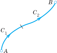
The curve C is called the path of integration. Look at Fig. 219a. The path of integration goes from A to B. Thus A: r(a) is its initial point and B: r(b) is its terminal point. C is now oriented. The direction from A to B, in which t increases is called the positive direction on C. We mark it by an arrow. The points A and B may coincide, as it happens in Fig. 219b. Then C is called a closed path.
C is called a smooth curve if it has at each point a unique tangent whose direction varies continuously as we move along C. We note that r(t) in (2) is differentiable. Its derivative r′(t) = dr/dt is continuous and different from the zero vector at every point of C.
General Assumption
In this book, every path of integration of a line integral is assumed to be piecewise smooth, that is, it consists of finitely many smooth curves.
For example, the boundary curve of a square is piecewise smooth. It consists of four smooth curves or, in this case, line segments which are the four sides of the square.
Definition and Evaluation of Line Integrals
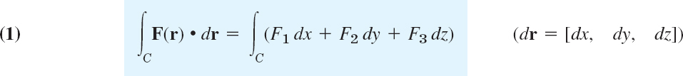
A line integral of a vector function F(r) over a curve C: r(t) is defined by
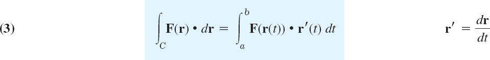
where r(t) is the parametric representation of C as given in (2). (The dot product was defined in Sec. 9.2.) Writing (3) in terms of components, with dr = [dx, dy, dz] as in Sec. 9.5 and ′ = d/dt, we get

If the path of integration C in (3) is a closed curve, then instead of
Note that the integrand in (3) is a scalar, not a vector, because we take the dot product. Indeed, F • r′/|r′| is the tangential component of F. (For “component” see (11) in Sec. 9.2.)
We see that the integral in (3) on the right is a definite integral of a function of t taken over the interval a ![]() t
t ![]() b on the t-axis in the positive direction: The direction of increasing t. This definite integral exists for continuous F and piecewise smooth C, because this makes F • r′ piecewise continuous.
b on the t-axis in the positive direction: The direction of increasing t. This definite integral exists for continuous F and piecewise smooth C, because this makes F • r′ piecewise continuous.
Line integrals (3) arise naturally in mechanics, where they give the work done by a force F in a displacement along C. This will be explained in detail below. We may thus call the line integral (3) the work integral. Other forms of the line integral will be discussed later in this section.
EXAMPLE 1 Evaluation of a Line Integral in the Plane
Find the value of the line integral (3) when F(r) = [−y, −xy] = −yi − xyj and C is the circular arc in Fig. 220 from A to B.
Solution. We may represent C by r(t) = [cos t, sin t] = cos t i + sin t j, where 0 ![]() t
t ![]() π/2. Then x(t) = cos t, y(t) = sin t, and
π/2. Then x(t) = cos t, y(t) = sin t, and
![]()
By differentiation, r′(t) = [−sin t, cos t] = −sin t i + cos t j, so that by (3) [use (10) in App. 3.1; set cos t = u in the second term]


Fig. 220. Example 1
EXAMPLE 2 Line Integral in Space
The evaluation of line integrals in space is practically the same as it is in the plane. To see this, find the value of (3) when F(r) = [z, x, y] = zi + xj + yk and C is the helix (Fig. 221)
![]()
Solution. From (4) we have x(t) = cos t, y(t) = sin t, z(t) = 3t. Thus
![]()
The dot product is 3t(−sin t) + cos2 t + 3 sin t. Hence (3) gives
![]()
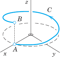
Fig. 221. Example 2
Simple general properties of the line integral (3) follow directly from corresponding properties of the definite integral in calculus, namely,


where in (5c) the path C is subdivided into two arcs C1 and C2 that have the same orientation as C (Fig. 222). In (5b) the orientation of C is the same in all three integrals. If the sense of integration along C is reversed, the value of the integral is multiplied by −1. However, we note the following independence if the sense is preserved.
THEOREM 1 Direction-Preserving Parametric Transformations
Any representations of C that give the same positive direction on C also yield the same value of the line integral (3).
PROOF
The proof follows by the chain rule. Let r(t) be the given representation with a ![]() t
t ![]() b as in (3). Consider the transformation t = φ(t*) which transforms the t interval to a*
b as in (3). Consider the transformation t = φ(t*) which transforms the t interval to a* ![]() t*
t* ![]() b* and has a positive derivative dt/dt*. We write r(t) = r(φ(t*)) = r*(t*). Then dt = (dt/dt*) dt* and
b* and has a positive derivative dt/dt*. We write r(t) = r(φ(t*)) = r*(t*). Then dt = (dt/dt*) dt* and

Motivation of the Line Integral (3): Work Done by a Force
The work W done by a constant force F in the displacement along a straight segment d is W = F • d; see Example 2 in Sec. 9.2. This suggests that we define the work W done by a variable force F in the displacement along a curve C: r(t) as the limit of sums of works done in displacements along small chords of C. We show that this definition amounts to defining W by the line integral (3).
For this we choose points t0 (=a) < t1 < … < tn (=b). Then the work ΔWm done by F(r(tm)) in the straight displacement from r(tm) to r(tm+1) is
![]()
The sum of these n works is Wn = Δ W0 + … + Δ Wn−1. If we choose points and consider Wn for every n arbitrarily but so that the greatest Δtm approaches zero as n → ∞ then the limit of Wn as n → ∞ is the line integral (3). This integral exists because of our general assumption that F is continuous and C is piecewise smooth; this makes r′(t) continuous, except at finitely many points where C may have corners or cusps.
EXAMPLE 3 Work Done by a Variable Force
If F in Example 1 is a force, the work done by F in the displacement along the quarter-circle is 0.4521, measured in suitable units, say, newton-meters (nt · m, also called joules, abbreviation J; see also inside front cover). Similarly in Example 2.
EXAMPLE 4 Work Done Equals the Gain in Kinetic Energy
Let F be a force, so that (3) is work. Let t be time, so that dr/dt = v, velocity. Then we can write (3) as

Now by Newton's second law, that is, force = mass × acceleration, we get
![]()
where m is the mass of the body displaced. Substitution into (5) gives [see (11), Sec. 9.4]

On the right, m|v|2/2 is the kinetic energy. Hence the work done equals the gain in kinetic energy. This is a basic law in mechanics.
Other Forms of Line Integrals
The line integrals
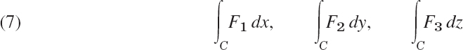
are special cases of (3) when F = F1i or F2j or F3k, respectively.
Furthermore, without taking a dot product as in (3) we can obtain a line integral whose value is a vector rather than a scalar, namely,
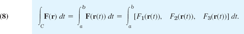
Obviously, a special case of (7) is obtained by taking F1 = f, F2 = F3 = 0. Then

with C as in (2). The evaluation is similar to that before.
EXAMPLE 5 A Line Integral of the Form (8)
Integrate F(r) = [xy, yz, z] along the helix in Example 2.
Solution. F(r(t)) = [cos t sin t, 3t sin t, 3t] integrated with respect to t from 0 to 2π gives

Path Dependence
Path dependence of line integrals is practically and theoretically so important that we formulate it as a theorem. And a whole section (Sec. 10.2) will be devoted to conditions under which path dependence does not occur.
The line integral (3) generally depends not only on F and on the endpoints A and B of the path, but also on the path itself along which the integral is taken.
PROOF
Almost any example will show this. Take, for instance, the straight segment C1: r1(t) = [t, t, 0] and the parabola C2: r2(t) = [t, t2, 0] with 0 ![]() t
t ![]() 1 (Fig. 223) and integrate F = [0, xy, 0]. Then
1 (Fig. 223) and integrate F = [0, xy, 0]. Then ![]() , so that integration gives 1/3 and 2/5, respectively.
, so that integration gives 1/3 and 2/5, respectively.

Fig. 223. Proof of Theorem 2
- WRITING PROJECT. From Definite Integrals to Line Integrals. Write a short report (1–2 pages) with examples on line integrals as generalizations of definite integrals. The latter give the area under a curve. Explain the corresponding geometric interpretation of a line integral.
2–11 LINE INTEGRAL. WORK
Calculate ![]() for the given data. If F is a force, this gives the work done by the force in the displacement along C. Show the details.
for the given data. If F is a force, this gives the work done by the force in the displacement along C. Show the details.
- 2. F = [y2, −x2], C: y = 4x2 from (0, 0) to (1, 4)
- 3. F as in Prob. 2, C from (0, 0) straight to (1, 4). Compare.
- 4. F = [xy, x2y2], C from (2, 0) straight to (0, 2)
- 5. F as in Prob. 4, C the quarter-circle from (2, 0) to (0, 2) with center (0, 0)
- 6. F = [x − y, y − z, z − x], C: r = [2 cos t, t, 2 sin t] from (2, 0, 0) to (2, 2π, 0)
- 7. F = [x2, y2, z2], C: r = [cos t, sin t, et] from (1, 0, 1) to (1, 0, e2π). Sketch C.
- 8. F = [ex, cosh y, sinh z], C: r = [t, t2, t3] from (0, 0, 0) to
 . Sketch C.
 - 9. F = [x + y, y + z, z + x], C: r = [2t, 5t, t] from t = 0 to 1. Also from t = −1 to 1.
- 10. F = [x, −z, 2y] from (0, 0, 0) straight to (1, 1, 0), then to (1, 1, 1), back to (0, 0, 0)
- 11. F = [e−x, e−y, e−z], C: r = [t, t2, t] from (0, 0, 0) to (2, 4, 2). Sketch C.
- 12. PROJECT. Change of Parameter. Path Dependence.
Consider the integral
 .
.(a) One path, several representations. Find the value of the integral when r = [cos t, sin t], 0
 t π/2. Show that the value remains the same if you set t = −p or t = p2 or apply two other parametric transformations of your own choice.
(b) Several paths. Evaluate the integral when C: y = xn, thus r = [t, tn], 0
t 1, where n = 1, 2, 3, …. Note that these infinitely many paths have the same endpoints.(c) Limit. What is the limit in (b) as n → ∞? Can you confirm your result by direct integration without referring to (b)?
(d) Show path dependence with a simple example of your choice involving two paths.
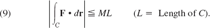
- 13. ML-Inequality, Estimation of Line Integrals. Let F be a vector function defined on a curve C. Let |F| be bounded, say, |F| M on C, where M is some positive number. Show that
- 14. Using (9), find a bound for the absolute value of the work W done by the force F = [x2, y] in the displacement from (0, 0) straight to (3, 4). Integrate exactly and compare.
15–20 INTEGRALS (8) AND (8*)
Evaluate them with F or f and C as follows.
- 15. F = [y2, z2, x2], C: r = [3 cos t, 3 sin t, 2t], 0 t 4π
- 16. f = 3x + y + 5z, C: r = [t, cosh t, sinh t], 0 t 1. Sketch C.
- 17. F = [x + y, y + z, z + x], C; r = [4 cos t, sin t, 0], 0 t π
- 18. F = [y1/3, x1/3, 0], C the hypocycloid r = [cos3 t, sin3 t, 0], 0 t π/4
- 19. f = xyz, C: r = [4t, 3t2, 12t], −2 t 2. Sketch C.
- 20. F = [xz, yz, x2y2], C: r = [t, t, et], 0 t 5. Sketch C.
10.2 Path Independence of Line Integrals
We want to find out under what conditions, in some domain, a line integral takes on the same value no matter what path of integration is taken (in that domain). As before we consider line integrals
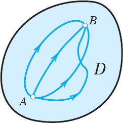
The line integral (1) is said to be path independent in a domain D in space if for every pair of endpoints A, B in domain D, (1) has the same value for all paths in D that begin at A and end at B. This is illustrated in Fig. 224. (See Sec. 9.6 for “domain.”)
Path independence is important. For instance, in mechanics it may mean that we have to do the same amount of work regardless of the path to the mountaintop, be it short and steep or long and gentle. Or it may mean that in releasing an elastic spring we get back the work done in expanding it. Not all forces are of this type—think of swimming in a big round pool in which the water is rotating as in a whirlpool.
We shall follow up with three ideas about path independence. We shall see that path independence of (1) in a domain D holds if and only if:
(Theorem 1) F = grad f, where grad f is the gradient of f as explained in Sec. 9.7.
(Theorem 2) Integration around closed curves C in D always gives 0.
(Theorem 3), curl F = 0, provided D is simply connected, as defined below.
Do you see that these theorems can help in understanding the examples and counterexample just mentioned?
Let us begin our discussion with the following very practical criterion for path independence.
A line integral (1) with continuous F1, F2, F3 in a domain D in space is path independent in D if and only if F = [F1, F2, F3] is the gradient of some function f in D,

PROOF
(a) We assume that (2) holds for some function f in D and show that this implies path independence. Let C be any path in D from any point A to any point B in D, given by r(t) = [x(t), y(t), z(t)], where a ![]() t
t ![]() b. Then from (2), the chain rule in Sec. 9.6, and (3′) in the last section we obtain
b. Then from (2), the chain rule in Sec. 9.6, and (3′) in the last section we obtain

(b) The more complicated proof of the converse, that path independence implies (2) for some f, is given in App. 4.
The last formula in part (a) of the proof,

is the analog of the usual formula for definite integrals in calculus,

Formula (3) should be applied whenever a line integral is independent of path.
Potential theory relates to our present discussion if we remember from Sec. 9.7 that when F = grad f, then f is called a potential of F. Thus the integral (1) is independent of path in D if and only if F is the gradient of a potential in D.
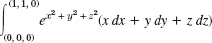
Show that the integral ![]() is path independent in any domain in space and find its value in the integration from A: (0, 0, 0) to B: (2, 2, 2).
is path independent in any domain in space and find its value in the integration from A: (0, 0, 0) to B: (2, 2, 2).
Solution. F = [2x, 2y, 4z] = grad f, where f = x2 + y2 + 2z2 because ∂f/∂x = 2x = F1, ∂f/∂y = 2y = F2, ∂f/∂z = 4z = F3. Hence the integral is independent of path according to Theorem 1, and (3) gives f(B) − f(A) = f(2, 2, 2) − f(0, 0, 0) = 4 + 4 + 8 = 16.
If you want to check this, use the most convenient path C: r(t) = [t, t, t], 0 ![]() t
t ![]() 2, on which F(r(t) = [2t, 2t, 4t], so that F(r(t)) • r′(t) = 2t + 2t + 4t = 8t, and integration from 0 to 2 gives 8 · 22/2 = 16.
2, on which F(r(t) = [2t, 2t, 4t], so that F(r(t)) • r′(t) = 2t + 2t + 4t = 8t, and integration from 0 to 2 gives 8 · 22/2 = 16.
If you did not see the potential by inspection, use the method in the next example.
EXAMPLE 2 Path Independence. Determination of a Potential
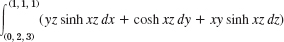
Evaluate the integral ![]() from A: (0, 1, 2) to B: (1, −1, 7) by showing that F has a potential and applying (3).
from A: (0, 1, 2) to B: (1, −1, 7) by showing that F has a potential and applying (3).
Solution. If F has a potential f, we should have
![]()
We show that we can satisfy these conditions. By integration of fx and differentiation,

This gives f(x, y, z) = x3 + y3z and by (3),
![]()
Path Independence and Integration Around Closed Curves
The simple idea is that two paths with common endpoints (Fig. 225) make up a single closed curve. This gives almost immediately
The integral (1) is path independent in a domain D if and only if its value around every closed path in D is zero.
PROOF
If we have path independence, then integration from A to B along C1 and along C2 in Fig. 225 gives the same value. Now C1 and C2 together make up a closed curve C, and if we integrate from A along C1 to B as before, but then in the opposite sense along C2 back to A (so that this second integral is multiplied by −1), the sum of the two integrals is zero, but this is the integral around the closed curve C.

Fig. 225. Proof of Theorem 2
Conversely, assume that the integral around any closed path C in D is zero. Given any points A and B and any two curves C1 and C2 from A to B in D, we see that C1 with the orientation reversed and C2 together form a closed path C. By assumption, the integral over C is zero. Hence the integrals over C1 and C2, both taken from A to B, must be equal. This proves the theorem.
Work. Conservative and Nonconservative (Dissipative) Physical Systems
Recall from the last section that in mechanics, the integral (1) gives the work done by a force F in the displacement of a body along the curve C. Then Theorem 2 states that work is path independent in D if and only if its value is zero for displacement around every closed path in D. Furthermore, Theorem 1 tells us that this happens if and only if F is the gradient of a potential in D. In this case, F and the vector field defined by F are called conservative in D because in this case mechanical energy is conserved; that is, no work is done in the displacement from a point A and back to A. Similarly for the displacement of an electrical charge (an electron, for instance) in a conservative electrostatic field.
Physically, the kinetic energy of a body can be interpreted as the ability of the body to do work by virtue of its motion, and if the body moves in a conservative field of force, after the completion of a round trip the body will return to its initial position with the same kinetic energy it had originally. For instance, the gravitational force is conservative; if we throw a ball vertically up, it will (if we assume air resistance to be negligible) return to our hand with the same kinetic energy it had when it left our hand.
Friction, air resistance, and water resistance always act against the direction of motion. They tend to diminish the total mechanical energy of a system, usually converting it into heat or mechanical energy of the surrounding medium (possibly both). Furthermore, if during the motion of a body, these forces become so large that they can no longer be neglected, then the resultant force F of the forces acting on the body is no longer conservative. This leads to the following terms. A physical system is called conservative if all the forces acting in it are conservative. If this does not hold, then the physical system is called nonconservative or dissipative.
Path Independence and Exactness of Differential Forms
Theorem 1 relates path independence of the line integral (1) to the gradient and Theorem 2 to integration around closed curves. A third idea (leading to Theorems 3* and 3, below) relates path independence to the exactness of the differential form or Pfaffian form1

under the integral sign in (1). This form (4) is called exact in a domain D in space if it is the differential

of a differentiable function f(x, y, z) everywhere in D, that is, if we have
![]()
Comparing these two formulas, we see that the form (4) is exact if and only if there is a differentiable function f(x, y, z) in D such that everywhere in D,

Hence Theorem 1 implies
The integral (1) is path independent in a domain D in space if and only if the differential form (4) has continuous coefficient functions F1, F2, F3 and is exact in D.
This theorem is of practical importance because it leads to a useful exactness criterion. First we need the following concept, which is of general interest.
A domain D is called simply connected if every closed curve in D can be continuously shrunk to any point in D without leaving D.
For example, the interior of a sphere or a cube, the interior of a sphere with finitely many points removed, and the domain between two concentric spheres are simply connected. On the other hand, the interior of a torus, which is a doughnut as shown in Fig. 249 in Sec. 10.6 is not simply connected. Neither is the interior of a cube with one space diagonal removed.
The criterion for exactness (and path independence by Theorem 3*) is now as follows.
THEOREM 3 Criterion for Exactness and Path Independence
Let F1, F2, F3 in the line integral (1),
be continuous and have continuous first partial derivatives in a domain D in space. Then:
(a) If the differential form (4) is exact in D—and thus (1) is path independent by Theorem 3*—, then in D,

in components (see Sec. 9.9)

(b) If (6) holds in D and D is simply connected, then (4) is exact in D—and thus (1) is path independent by Theorem 3*.
PROOF
(a) If (4) is exact in D, then F = grad f in D by Theorem 3*, and, furthermore, curl F = curl (grad f) = 0 by (2) in Sec. 9.9, so that (6) holds.
(b) The proof needs “Stokes's theorem” and will be given in Sec. 10.9.
Line Integral in the Plane. For ![]() the curl has only one component (the z-component), so that (6′) reduces to the single relation
the curl has only one component (the z-component), so that (6′) reduces to the single relation

(which also occurs in (5) of Sec. 1.4 on exact ODEs).
EXAMPLE 3 Exactness and Independence of Path. Determination of a Potential
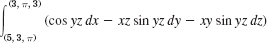
Using (6′), show that the differential form under the integral sign of
![]()
is exact, so that we have independence of path in any domain, and find the value of I from A: (0, 0, 1) to B: (1, π/4, 2).
Solution. Exactness follows from (6′), which gives

To find f, we integrate F2 (which is “long,” so that we save work) and then differentiate to compare with F1 and F3,

h′ = 0 implies h = const and we can take h = 0, so that g = 0 in the first line. This gives, by (3),
![]()
The assumption in Theorem 3 that D is simply connected is essential and cannot be omitted. Perhaps the simplest example to see this is the following.
EXAMPLE 4 On the Assumption of Simple Connectedness in Theorem 3
Let

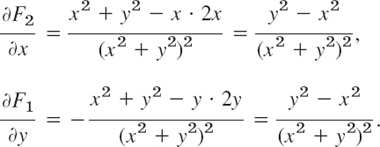
Differentiation shows that (6′) is satisfied in any domain of the xy-plane not containing the origin, for example, in the domain ![]() shown in Fig. 226. Indeed, F1 and F2 do not depend on z, and F3 = 0, so that the first two relations in (6′) are trivially true, and the third is verified by differentiation:
shown in Fig. 226. Indeed, F1 and F2 do not depend on z, and F3 = 0, so that the first two relations in (6′) are trivially true, and the third is verified by differentiation:
Clearly, D in Fig. 226 is not simply connected. If the integral

were independent of path in D, then I = 0 on any closed curve in D, for example, on the circle x2 + y2 = 1. But setting x = r cos θ, y = r sin θ and noting that the circle is represented by r = 1, we have
![]()
so that −y dx + x dy = sin2 θ dθ + cos2 θ dθ = dθ and counterclockwise integration gives

Since D is not simply connected, we cannot apply Theorem 3 and cannot conclude that I is independent of path in D.
Although F = grad f, where f = arctan (y/x) (verify!), we cannot apply Theorem 1 either because the polar angle f = θ = arctan (y/x) is not single-valued, as it is required for a function in calculus.
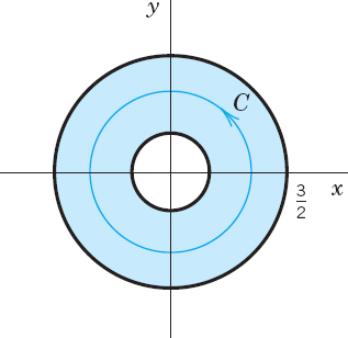
Fig. 226. Example 4
- WRITING PROJECT. Report on Path Independence. Make a list of the main ideas and facts on path independence and dependence in this section. Then work this list into a report. Explain the definitions and the practical usefulness of the theorems, with illustrative examples of your own. No proofs.
- On Example 4. Does the situation in Example 4 of the text change if you take the domain
 3/2?
3/2?
3–9 PATH INDEPENDENT INTEGRALS
Show that the form under the integral sign is exact in the plane (Probs. 3–4) or in space (Probs. 5–9) and evaluate the integral. Show the details of your work.
- 3.
- 4.

- 5.
- 6.
- 7.
- 8.
- 9.
- 10. PROJECT. Path Dependence. (a) Show that
 is path dependent in the xy-plane.
(b) Integrate from (0, 0) along the straight-line segment to (1, b), 0
b 1, and then vertically up to (1, 1); see the figure. For which b is I maximum? What is its maximum value?(c) Integrate I from (0, 0) along the straight-line segment to (c, 1), 0
c 1, and then horizontally to (1, 1). For c = 1, do you get the same value as for b = 1 in (b)? For which c is I maximum? What is its maximum value?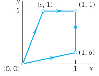
Project 10. Path Dependence
- 11. On Example 4. Show that in Example 4 of the text, F = grad (arctan (y/x)). Give examples of domains in which the integral is path independent.
- 12. CAS EXPERIMENT. Extension of Project 10. Integrate x2y dx + 2xy2 dy over various circles through the points (0, 0) and (1, 1). Find experimentally the smallest value of the integral and the approximate location of the center of the circle.
13–19 PATH INDEPENDENCE?
Check, and if independent, integrate from (0, 0, 0) to (a, b, c).
- 13.

- 14. (sinh xy) (z dx − x dz)
- 15. x2y dx − 4xy2 dy + 8z2x dz
- 16. ey dx + (xey − ez) dy − yez dz
- 17. 4y dx + z dy + (y − 2z)dz
- 18. (cos xy)(yz dx + xz dy) − 2 sin xy dz
- 19. (cos (x2 + 2y2 + z2))(2x dx + 4y dy + 2z dz)
- 20. Path Dependence. Construct three simple examples in each of which two equations (6′) are satisfied, but the third is not.
10.3 Calculus Review: Double Integrals. Optional
This section is optional. Students familiar with double integrals from calculus should skip this review and go on to Sec. 10.4. This section is included in the book to make it reasonably self-contained.
In a definite integral (1), Sec. 10.1, we integrate a function f(x) over an interval (a segment) of the x-axis. In a double integral we integrate a function f(x, y), called the integrand, over a closed bounded region2 R in the xy-plane, whose boundary curve has a unique tangent at almost every point, but may perhaps have finitely many cusps (such as the vertices of a triangle or rectangle).
The definition of the double integral is quite similar to that of the definite integral. We subdivide the region R by drawing parallels to the x- and y-axes (Fig. 227). We number the rectangles that are entirely within R from 1 to n. In each such rectangle we choose a point, say, (xk, yk) in the kth rectangle, whose area we denote by ΔAk. Then we form the sum


Fig. 227. Subdivision of a region R
This we do for larger and larger positive integers n in a completely independent manner, but so that the length of the maximum diagonal of the rectangles approaches zero as n approaches infinity. In this fashion we obtain a sequence of real numbers ![]() . Assuming that f(x, y) is continuous in R and R is bounded by finitely many smooth curves (see Sec. 10.1), one can show (see Ref. [GenRef4] in App. 1) that this sequence converges and its limit is independent of the choice of subdivisions and corresponding points (xk, yk). This limit is called the double integral of f(x, y) over the region R, and is denoted by
. Assuming that f(x, y) is continuous in R and R is bounded by finitely many smooth curves (see Sec. 10.1), one can show (see Ref. [GenRef4] in App. 1) that this sequence converges and its limit is independent of the choice of subdivisions and corresponding points (xk, yk). This limit is called the double integral of f(x, y) over the region R, and is denoted by
Double integrals have properties quite similar to those of definite integrals. Indeed, for any functions f and g of (x, y), defined and continuous in a region R,

Furthermore, if R is simply connected (see Sec. 10.2), then there exists at least one point (x0, y0) in R such that we have

where A is the area of R. This is called the mean value theoremfor double integrals.

Evaluation of Double Integrals by Two Successive Integrations
Double integrals over a region R may be evaluated by two successive integrations. We may integrate first over y and then over x. Then the formula is
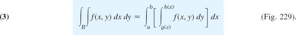
Here y = g(x) and y = h(x) represent the boundary curve of R (see Fig. 229) and, keeping x constant, we integrate f(x, y) over y from g(x) to h(x). The result is a function of x, and we integrate it from x = a to x = b (Fig. 229).
Similarly, for integrating first over x and then over y the formula is


Fig. 229. Evaluation of a double integral

Fig. 230. Evaluation of a double integral
The boundary curve of R is now represented by x = p(y) and x = q(y). Treating y as a constant, we first integrate f(x, y) over x from p(y) to q(y) (see Fig. 230) and then the resulting function of y from y = c to y = d.
In (3) we assumed that R can be given by inequalities a ![]() x
x ![]() b and g(x)
b and g(x) ![]() y
y ![]() h(x). Similarly in (4) by c
h(x). Similarly in (4) by c ![]() y
y ![]() d and p(y)
d and p(y) ![]() x
x ![]() q(y). If a region R has no such representation, then, in any practical case, it will at least be possible to subdivide R into finitely many portions each of which can be given by those inequalities. Then we integrate f(x, y) over each portion and take the sum of the results. This will give the value of the integral of f(x, y) over the entire region R.
q(y). If a region R has no such representation, then, in any practical case, it will at least be possible to subdivide R into finitely many portions each of which can be given by those inequalities. Then we integrate f(x, y) over each portion and take the sum of the results. This will give the value of the integral of f(x, y) over the entire region R.
Applications of Double Integrals
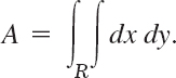
Double integrals have various physical and geometric applications. For instance, the area A of a region R in the xy-plane is given by the double integral
The volume V beneath the surface z = f(x, y)(> 0) and above a region R in the xy-plane is (Fig. 231)

because the term f(xk, yk)ΔAk in jn at the beginning of this section represents the volume of a rectangular box with base of area ΔAk and altitude f(xk, yk).

Fig. 231. Double integral as volume
As another application, let f(x, y) be the density (= mass per unit area) of a distribution of mass in the xy-plane. Then the total mass M in R is

the center of gravity of the mass in R has the coordinates ![]() , where
, where

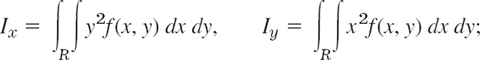
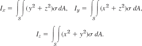
the moments of inertia Ix and Iy of the mass in R about the x- and y-axes, respectively, are
and the polar moment of inertia I0 about the origin of the mass in R is

An example is given below.
Change of Variables in Double Integrals. Jacobian
Practical problems often require a change of the variables of integration in double integrals. Recall from calculus that for a definite integral the formula for the change from x to u is

Here we assume that x = x(u) is continuous and has a continuous derivative in some interval α ![]() u
u ![]() β such that x(α) = a, x(β) = b[or x(α) = b, x(β) = a] and x(u) varies between a and b when u varies between α and β.
β such that x(α) = a, x(β) = b[or x(α) = b, x(β) = a] and x(u) varies between a and b when u varies between α and β.
The formula for a change of variables in double integrals from x, y to u, v is
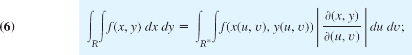
that is, the integrand is expressed in terms of u and υ, and dx dy is replaced by du dυ times the absolute value of the Jacobian3
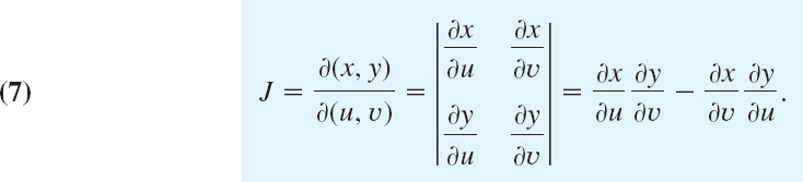
Here we assume the following. The functions
![]()
effecting the change are continuous and have continuous partial derivatives in some region R* in the uυ-plane such that for every (u, υ) in R* the corresponding point (x, y) lies in R and, conversely, to every (x, y) in R there corresponds one and only one (u, υ) in R*; furthermore, the Jacobian J is either positive throughout R* or negative throughout R*. For a proof, see Ref. [GenRef4] in App. 1.
EXAMPLE 1 Change of Variables in a Double Integral
Evaluate the following double integral over the square R in Fig. 232.
![]()
Solution. The shape of R suggests the transformation x + y = u, x − y = υ. Then ![]() ,
, ![]() . The Jacobian is
. The Jacobian is

R corresponds to the square 0 ![]() u
u ![]() 2, 0
2, 0 ![]() υ
υ ![]() 2. Therefore,
2. Therefore,
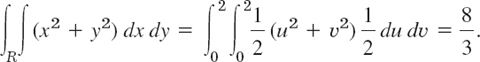

Fig. 232. Region R in Example 1
Of particular practical interest are polar coordinates r and θ, which can be introduced by setting x = r cos θ, y = r sin θ. Then
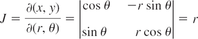
and
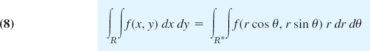
where R* is the region in the rθ-plane corresponding to R in the xy-plane.
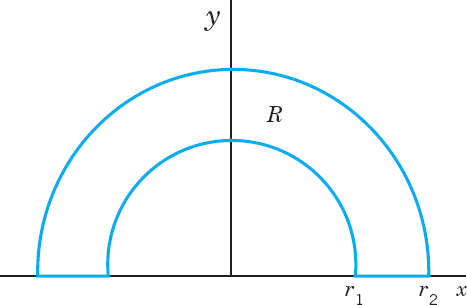
EXAMPLE 2 Double Integrals in Polar Coordinates. Center of Gravity. Moments of Inertia
Let f(x, y) = 1 be the mass density in the region in Fig. 233. Find the total mass, the center of gravity, and the moments of inertia Ix, Iy, I0.
Solution. We use the polar coordinates just defined and formula (8). This gives the total mass
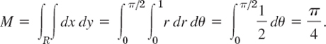

Fig. 233. Example 2
The center of gravity has the coordinates
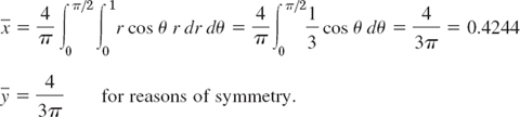
The moments of inertia are
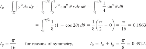
Why are ![]() and
and ![]() less than
less than ![]() ?
?
This is the end of our review on double integrals. These integrals will be needed in this chapter, beginning in the next section.
- Mean value theorem. Illustrate (2) with an example.
2–8 DOUBLE INTEGRALS
Describe the region of integration and evaluate.
- 2.
- 3.

- 4. Prob. 3, order reversed.
- 5.
- 6.
- 7. Prob. 6, order reversed.
- 8.
9–11 VOLUME
Find the volume of the given region in space.
- 9. The region beneath z = 4x2 + 9y2 and above the rectangle with vertices (0, 0), (3, 0), (3, 2), (0, 2) in the xy-plane.
- 10. The first octant region bounded by the coordinate planes and the surfaces y = 1 − x2, z = 1 − x2. Sketch it.
- 11. The region above the xy-plane and below the paraboloid z = 1 − (x2 + y2).
12–16 CENTER OF GRAVITY
Find the center of gravity ![]() of a mass of density f(x, y) = 1 in the given region R.
of a mass of density f(x, y) = 1 in the given region R.
- 12.

- 13.

- 14.
- 15.

- 16.

17–20 MOMENTS OF INERTIA
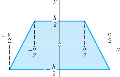
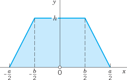
Find Ix, Iy, I0 of a mass of density f(x, y) = 1 in the region R in the figures, which the engineer is likely to need, along with other profiles listed in engineering handbooks.
- 17. R as in Prob. 13.
- 18. R as in Prob. 12.
- 19.
- 20.
10.4 Green's Theorem in the Plane
Double integrals over a plane region may be transformed into line integrals over the boundary of the region and conversely. This is of practical interest because it may simplify the evaluation of an integral. It also helps in theoretical work when we want to switch from one kind of integral to the other. The transformation can be done by the following theorem.
THEOREM 1 Green's Theorem in the Plane4 (Transformation between Double Integrals and Line Integrals)
Let R be a closed bounded region (see Sec. 10.3) in the xy-plane whose boundary C consists of finitely many smooth curves (see Sec. 10.1). Let F1(x, y) and F2(x, y) be functions that are continuous and have continuous partial derivatives ∂F1/∂y and ∂F2/∂x everywhere in some domain containing R. Then

Here we integrate along the entire boundary C of R in such a sense that R is on the left as we advance in the direction of integration (see Fig. 234).

Fig. 234. Region R whose boundary C consists of two parts: C1 is traversed counterclockwise, while C2 is traversed clockwise in such a way that R is on the left for both curves
Setting F = [F1, F2] = F1i + F2j and using (1) in Sec. 9.9, we obtain (1) in vectorial form,

The proof follows after the first example. For ![]() see Sec. 10.1.
see Sec. 10.1.
EXAMPLE 1 Verification of Green's Theorem in the Plane
Green's theorem in the plane will be quite important in our further work. Before proving it, let us get used to it by verifying it for F1 = y2 − 7y, F2 = 2xy + 2x and C the circle x2 + y2 = 1.
Solution. In (1) on the left we get

since the circular disk R has area π.
We now show that the line integral in (1) on the right gives the same value, 9π. We must orient C counterclockwise, say, r(t) = [cos t, sin t]. Then r′(t) = [−sin t, cos t], and on C,
![]()
Hence the line integral in (1) becomes, verifying Green's theorem,

PROOF
We prove Green's theorem in the plane, first for a special region R that can be represented in both forms
![]()
and
![]()
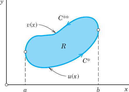
Fig. 235. Example of a special region

Fig. 236. Example of a special region
Using (3) in the last section, we obtain for the second term on the left side of (1) taken without the minus sign

(The first term will be considered later.) We integrate the inner integral:
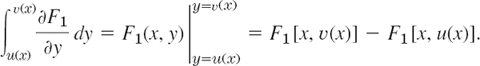
By inserting this into (2) we find (changing a direction of integration)
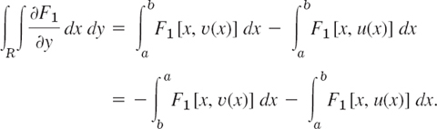
Since y = υ(x) represents the curve C** (Fig. 235) and y = u(x) represents C*, the last two integrals may be written as line integrals over C** and C* (oriented as in Fig. 235); therefore,

This proves (1) in Green's theorem if F2 = 0.
The result remains valid if C has portions parallel to the y-axis (such as ![]() and
and ![]() in Fig. 237). Indeed, the integrals over these portions are zero because in (3) on the right we integrate with respect to x. Hence we may add these integrals to the integrals over C* and C** to obtain the integral over the whole boundary C in (3).
in Fig. 237). Indeed, the integrals over these portions are zero because in (3) on the right we integrate with respect to x. Hence we may add these integrals to the integrals over C* and C** to obtain the integral over the whole boundary C in (3).
We now treat the first term in (1) on the left in the same way. Instead of (3) in the last section we use (4), and the second representation of the special region (see Fig. 236). Then (again changing a direction of integration)

Together with (3) this gives (1) and proves Green's theorem for special regions.
We now prove the theorem for a region R that itself is not a special region but can be subdivided into finitely many special regions as shown in Fig. 238. In this case we apply the theorem to each subregion and then add the results; the left-hand members add up to the integral over R while the right-hand members add up to the line integral over C plus integrals over the curves introduced for subdividing R. The simple key observation now is that each of the latter integrals occurs twice, taken once in each direction. Hence they cancel each other, leaving us with the line integral over C.
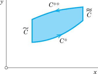
Fig. 237. Proof of Green's theorem

Fig. 238. Proof of Green's theorem
The proof thus far covers all regions that are of interest in practical problems. To prove the theorem for a most general region R satisfying the conditions in the theorem, we must approximate R by a region of the type just considered and then use a limiting process. For details of this see Ref. [GenRef4] in App. 1.
Some Applications of Green's Theorem
EXAMPLE 2 Area of a Plane Region as a Line Integral Over the Boundary
In (1) we first choose F1 = 0, F2 = x and then F1 = −y, F2 = 0. This gives

respectively. The double integral is the area A of R. By addition we have

where we integrate as indicated in Green's theorem. This interesting formula expresses the area of R in terms of a line integral over the boundary. It is used, for instance, in the theory of certain planimeters (mechanical instruments for measuring area). See also Prob. 11.
For an ellipse x2/a2 + y2/b2 = 1 or x = a cos t, y = b sin t we get x′ = −a sin t, y′ = b cos t; thus from (4) we obtain the familiar formula for the area of the region bounded by an ellipse,
![]()
EXAMPLE 3 Area of a Plane Region in Polar Coordinates
Let r and θ be polar coordinates defined by x = r cos θ, y = r sin θ. Then
![]()
and (4) becomes a formula that is well known from calculus, namely,

As an application of (5), we consider the cardioid r = a(1 − cos θ), where 0 ![]() θ
θ ![]() 2π (Fig. 239). We find
2π (Fig. 239). We find
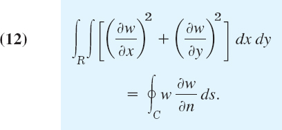
EXAMPLE 4 Transformation of a Double Integral of the Laplacian of a Function into a Line Integral of Its Normal Derivative
The Laplacian plays an important role in physics and engineering. A first impression of this was obtained in Sec. 9.7, and we shall discuss this further in Chap. 12. At present, let us use Green's theorem for deriving a basic integral formula involving the Laplacian.
We take a function w(x, y) that is continuous and has continuous first and second partial derivatives in a domain of the xy-plane containing a region R of the type indicated in Green's theorem. We set F1 = −∂w/∂y and F2 = ∂w/∂x. Then ∂F1/∂y and ∂F2/∂x are continuous in R, and in (1) on the left we obtain

the Laplacian of w (see Sec. 9.7). Furthermore, using those expressions for F1 and F2, we get in (1) on the right

where s is the arc length of C, and C is oriented as shown in Fig. 240. The integrand of the last integral may be written as the dot product

The vector n is a unit normal vector to C, because the vector r′ (s) = dr/ds = [dx/ds, dy/ds] is the unit tangent vector of C, and r′ • n = 0, so that n is perpendicular to r′. Also, n is directed to the exterior of C because in Fig. 240 the positive x-component dx/ds of r′ is the negative y-component of n, and similarly at other points. From this and (4) in Sec. 9.7 we see that the left side of (8) is the derivative of w in the direction of the outward normal of C. This derivative is called the normal derivative of w and is denoted by ∂w/∂n; that is, ∂w/∂n = (grad w) • n. Because of (6), (7), and (8), Green's theorem gives the desired formula relating the Laplacian to the normal derivative,

For instance, w = x2 − y2 satisfies Laplace's equation ∇2w = 0. Hence its normal derivative integrated over a closed curve must give 0. Can you verify this directly by integration, say, for the square 0 ![]() x
x ![]() 1, 0
1, 0 ![]() y
y ![]() 1?
1?


Fig. 240. Example 4
Green's theorem in the plane can be used in both directions, and thus may aid in the evaluation of a given integral by transforming the given integral into another integral that is easier to solve. This is illustrated further in the problem set. Moreover, and perhaps more fundamentally, Green's theorem will be the essential tool in the proof of a very important integral theorem, namely, Stokes's theorem in Sec. 10.9.
1–10 LINE INTEGRALS: EVALUATION BY GREEN'S THEOREM
Evaluate ![]() counterclockwise around the boundary C of the region R by Green's theorem, where
counterclockwise around the boundary C of the region R by Green's theorem, where
- F = [y, −x], C the circle x2 + y2 = 1/4
- F = [6y2, 2x − 2y4], R the square with vertices ±(2, 2), ±(2, −2)
- F = [x2ey, y2, ex], R the rectangle with vertices (0, 0), (2, 0), (2, 3), (0, 3)
- F = [x cosh 2y, 2x2 sinh 2y], R: x2 y x
- F = [x2 + y2, x2 − y2], R: 1 y 2 − x2
- F = [cosh y, −sinh x], R: 1 x 3, x y 3x
- F = grad (x3 cos2 (xy)), R as in Prob. 5
- F = [−e−x cos y, −e−x sin y], R the semidisk x2 + y2 16, x
 0
0 - F = [ey/x, ey ln x + 2x], R: 1 + x4 y 2
- F = [x2y, −x/y2], R: 1 x2 + y2 4, x 0, y x. Sketch R.
- CAS EXPERIMENT. Apply (4) to figures of your choice whose area can also be obtained by another method and compare the results.
- PROJECT. Other Forms of Green's Theorem in the Plane. Let R and C be as in Green's theorem, r′ a unit tangent vector, and n the outer unit normal vector of C (Fig. 240 in Example 4). Show that (1) may be written

or

where k is a unit vector perpendicular to the xy-plane. Verify (10) and (11) for F = [7x, −3y] and C the circle x2 + y2 = 4 as well as for an example of your own choice.
13–17 INTEGRAL OF THE NORMAL DERIVATIVE
Using (9), find the value of ![]() taken counterclockwise over the boundary C of the region R.
taken counterclockwise over the boundary C of the region R.
- 13. w = cosh x, R the triangle with vertices (0, 0), (4, 2), (0, 2).
- 14. w = x2y + xy2, R: x2 + y2 1, x 0, y 0
- 15. w = ex cos y + xy3, R: 1 y 10 − x2, x 0
- 16. W = x2 + y2, C; x2 + y2 = 4. Confirm the answer by direct integration.
- 17. w = x3 − y3, 0 y x2, |x| 2
- 18. Laplace's equation. Show that for a solution w(x, y) of Laplace's equation ∇2w = 0 in a region R with boundary curve C and outer unit normal vector n,
- 19. Show that w = ex sin y satisfies Laplace's equation ∇2w = 0 and, using (12), integrate w(∂w/∂n) counterclockwise around the boundary curve C of the rectangle 0 x 2, 0 y 5.
- 20. Same task as in Prob. 19 when w = x2 + y2 and C the boundary curve of the triangle with vertices (0, 0), (1, 0), (0, 1).
10.5 Surfaces for Surface Integrals
Whereas, with line integrals, we integrate over curves in space (Secs. 10.1, 10.2), with surface integrals we integrate over surfaces in space. Each curve in space is represented by a parametric equation (Secs. 9.5, 10.1). This suggests that we should also find parametric representations for the surfaces in space. This is indeed one of the goals of this section. The surfaces considered are cylinders, spheres, cones, and others. The second goal is to learn about surface normals. Both goals prepare us for Sec. 10.6 on surface integrals. Note that for simplicity, we shall say “surface” also for a portion of a surface.
Representation of Surfaces
Representations of a surface S in xyz-space are
![]()
For example, ![]() or x2 + y2 + z2 − a2 = 0 (z
or x2 + y2 + z2 − a2 = 0 (z ![]() 0) represents a hemisphere of radius a and center 0.
0) represents a hemisphere of radius a and center 0.
Now for curves C in line integrals, it was more practical and gave greater flexibility to use a parametric representation r = r(t), where a ![]() t
t ![]() b. This is a mapping of the interval a
b. This is a mapping of the interval a ![]() t
t ![]() b, located on the t-axis, onto the curve C (actually a portion of it) in xyz-space. It maps every t in that interval onto the point of C with position vector r(t). See Fig. 241A.
b, located on the t-axis, onto the curve C (actually a portion of it) in xyz-space. It maps every t in that interval onto the point of C with position vector r(t). See Fig. 241A.
Similarly, for surfaces S in surface integrals, it will often be more practical to use a parametric representation. Surfaces are two-dimensional. Hence we need two parameters, which we call u and υ. Thus a parametric representation of a surface S in space is of the form
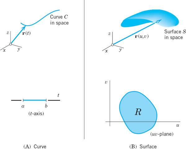
Fig. 241. Parametric representations of a curve and a surface

where (u, υ) varies in some region R of the uυ-plane. This mapping (2) maps every point (u, υ) in R onto the point of S with position vector r(u, υ). See Fig. 241B.
EXAMPLE 1 Parametric Representation of a Cylinder
The circular cylinder x2 + y2 = a2, −1 ![]() z
z ![]() 1, has radius a, height 2, and the z-axis as axis. A parametric representation is
1, has radius a, height 2, and the z-axis as axis. A parametric representation is
![]()
The components of r are x = a cos u, y = a sin u, z = υ. The parameters u, υ vary in the rectangle R; 0 ![]() u
u ![]() 2π, −1
2π, −1 ![]() υ
υ ![]() 1 in the uυ-plane. The curves u = const are vertical straight lines. The curves υ = const are parallel circles. The point P in Fig. 242 corresponds to u = π/3 = 60°, υ = 0.7.
1 in the uυ-plane. The curves u = const are vertical straight lines. The curves υ = const are parallel circles. The point P in Fig. 242 corresponds to u = π/3 = 60°, υ = 0.7.
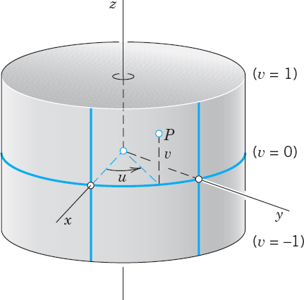
Fig. 242. Parametric representation
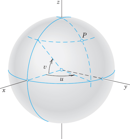
Fig. 243. Parametric representation of a cylinder of a sphere
EXAMPLE 2 Parametric Representation of a Sphere
A sphere x2 + y2 + z2 = a2 can be represented in the form

where the parameters u, υ vary in the rectangle R in the uυ-plane given by the inequalities 0 ![]() u
u ![]() 2π, −π/2
2π, −π/2 ![]() υ
υ ![]() π/2. The components of r are
π/2. The components of r are
![]()
The curves u = const and υ = const are the “meridians” and “parallels” on S (see Fig. 243). This representation is used ingeography for measuring the latitude and longitude of points on the globe.
Another parametric representation of the sphere also used in mathematics is

where 0 ![]() u
u ![]() 2π, 0
2π, 0 ![]() υ
υ ![]() π.
π.
EXAMPLE 3 Parametric Representation of a Cone
A circular cone ![]() can be represented by
can be represented by
![]()
in components x = u cos υ, y = u sin υ, z = u. The parameters vary in the rectangle R: 0 ![]() u
u ![]() H, 0
H, 0 ![]() υ
υ ![]() 2π. Check that x2 + y2 = z2, as it should be. What are the curves u = const and υ = const?
2π. Check that x2 + y2 = z2, as it should be. What are the curves u = const and υ = const?
Tangent Plane and Surface Normal
Recall from Sec. 9.7 that the tangent vectors of all the curves on a surface S through a point P of S form a plane, called the tangent plane of S at P (Fig. 244). Exceptions are points where S has an edge or a cusp (like a cone), so that S cannot have a tangent plane at such a point. Furthermore, a vector perpendicular to the tangent plane is called a normal vector of S at P.
Now since S can be given by r = r(u, υ) in (2), the new idea is that we get a curve C on S by taking a pair of differentiable functions
![]()
whose derivatives u′ = du/dt and υ′ = dυ/dt are continuous. Then C has the position vector ![]() . By differentiation and the use of the chain rule (Sec. 9.6) we obtain a tangent vector of C on S
. By differentiation and the use of the chain rule (Sec. 9.6) we obtain a tangent vector of C on S

Hence the partial derivatives ru and rυ at P are tangential to S at P. We assume that they are linearly independent, which geometrically means that the curves u = const and υ = const on S intersect at P at a nonzero angle. Then ru and rυ span the tangent plane of S at P. Hence their cross product gives a normal vector N of S at P.

The corresponding unit normal vector n of S at P is (Fig. 244)


Fig. 244. Tangent plane and normal vector
Also, if S is represented by g(x, y, z) = 0, then, by Theorem 2 in Sec. 9.7,

A surface S is called a smooth surface if its surface normal depends continuously on the points of S.
S is called piecewise smooth if it consists of finitely many smooth portions.
For instance, a sphere is smooth, and the surface of a cube is piecewise smooth (explain!). We can now summarize our discussion as follows.
THEOREM 1 Tangent Plane and Surface Normal
If a surface S is given by (2) with continuous ru = ∂r/∂u and rυ = ∂r/∂υ satisfying (4) at every point of S, then S has, at every point P, a unique tangent plane passing through P and spanned by ru and rυ, and a unique normal whose direction depends continuously on the points of S. A normal vector is given by (4) and the corresponding unit normal vector by (5). (See Fig. 244.)
EXAMPLE 4 Unit Normal Vector of a Sphere
From (5*) we find that the sphere g(x, y, z) = x2 + y2 + z2 − a2 = 0 has the unit normal vector

We see that n has the direction of the position vector [x, y, z] of the corresponding point. Is it obvious that this must be the case?
EXAMPLE 5 Unit Normal Vector of a Cone
At the apex of the cone ![]() in Example 3, the unit normal vector n becomes undetermined because from (5*) we get
in Example 3, the unit normal vector n becomes undetermined because from (5*) we get

We are now ready to discuss surface integrals and their applications, beginning in the next section.
1–8 PARAMETRIC SURFACE REPRESENTATION
Familiarize yourself with parametric representations of important surfaces by deriving a representation (1), by finding the parameter curves (curves u = const and υ = const) of the surface and a normal vector N = ru × rυ of the surface. Show the details of your work.
- xy-plane r(u, υ) = (u, υ) (thus ui + υj; similarly in Probs. 2–8).
- xy-plane in polar coordinates r(u, υ) = [u cos υ, u sin υ] (thus u = r, υ = θ)
- Cone r(u, υ) = [u cos υ, u sin υ, cu]
- Elliptic cylinder r(u, υ) = [a cos υ, b sin υ, u]
- Paraboloid of revolution r(u, υ) = [u cos υ, u sin υ, υ2]
- Helicoid r(u, υ) = [u cos υ, u sin υ, υ]. Explain the name.
- Ellipsoid r(u, υ) = [a cos υ cos u, b cos υ sin u, c sin υ]
- Hyperbolic paraboloid r(u, υ) = [au cosh υ, bu sinh υ, u2]
- CAS EXPERIMENT. Graphing Surfaces, Dependence on a, b, c. Graph the surfaces in Probs. 3–8. In Prob. 6 generalize the surface by introducing parameters a, b. Then find out in Probs. 4 and 6–8 how the shape of the surfaces depends on a, b, c.
- Orthogonal parameter curves u = const and υ = const on r(u, υ) occur if and only if ru • rυ = 0. Give examples. Prove it.
- Satisfying (4). Represent the paraboloid in Prob. 5 so that
 and show
  .
. - Condition (4). Find the points in Probs. 1–8 at which (4) N ≠ 0 does not hold. Indicate whether this results from the shape of the surface or from the choice of the representation.
- Representation z = f(x, y). Show that z = f(x, y) or g = z − f(x, y) = 0 can be written (fu = ∂f/∂u etc.)

14–19 DERIVE A PARAMETRIC REPRESENTATION
Find a normal vector. The answer gives one representation; there are many. Sketch the surface and parameter curves.
- 14. Plane 4x + 3y + 2z = 12
- 15. Cylinder of revolution (x − 2)2 + (y + 1)2 = 25
- 16. Ellipsoid

- 17. Sphere x2 + (y + 2.8)2 + (z − 3.2)2 = 2.25
- 18. Elliptic cone

- 19. Hyperbolic cylinder x2 − y2 = 1
- 20. PROJECT. Tangent Planes T(P) will be less important in our work, but you should know how to represent them.
(a) If S: r(u, υ), then T(P): (r* − r ru rυ) = 0 (a scalar triple product) or

(b) If S: g(x, y, z) = 0, then

(c) If S: z = f(x, y), then

Interpret (a)−(c) geometrically. Give two examples for (a), two for (b), and two for (c).
10.6 Surface Integrals
To define a surface integral, we take a surface S, given by a parametric representation as just discussed,
![]()
where (u, υ) varies over a region R in the uυ-plane. We assume S to be piecewise smooth (Sec. 10.5), so that S has a normal vector

at every point (except perhaps for some edges or cusps, as for a cube or cone). For a given vector function F we can now define the surface integral over S by
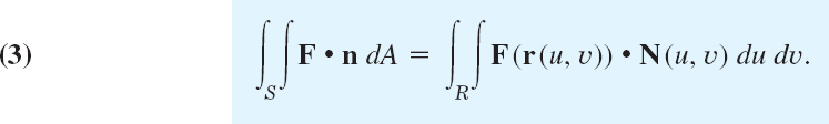
Here N = |N|n by (2), and |N| = |ru × rυ| is the area of the parallelogram with sides ru and rυ, by the definition of cross product. Hence

And we see that dA = |N|du dυ is the element of area of S.
Also F • n is the normal component of F. This integral arises naturally in flow problems, where it gives the flux across S when F = ρv. Recall, from Sec. 9.8, that the flux across S is the mass of fluid crossing S per unit time. Furthermore, ρ is the density of the fluid and v the velocity vector of the flow, as illustrated by Example 1 below. We may thus call the surface integral (3) the flux integral.
We can write (3) in components, using F = [F1, F2, F3], N = [N1, N2, N3], and n = [cos α, cos β, cos γ]. Here, α, β, γ are the angles between n and the coordinate axes; indeed, for the angle between n and i, formula (4) in Sec. 9.2 gives cos α = n • i/|n||i| = n • i, and so on. We thus obtain from (3)
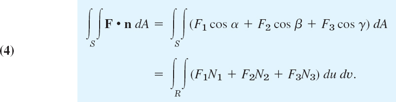
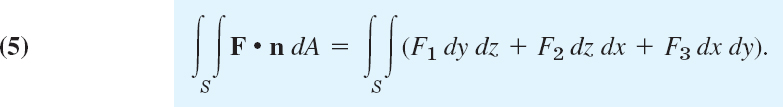
In (4) we can write cos α dA = dy dz, cos β dA = dz dx, cos γ dA = dx dy. Then (4) becomes the following integral for the flux:
We can use this formula to evaluate surface integrals by converting them to double integrals over regions in the coordinate planes of the xyz-coordinate system. But we must carefully take into account the orientation of S (the choice of n). We explain this for the integrals of the F3-terms,

If the surface S is given by z = h(x, y) with (x, y) varying in a region ![]() in the xy-plane, and if S is oriented so that cos γ > 0, then (5′) gives
in the xy-plane, and if S is oriented so that cos γ > 0, then (5′) gives
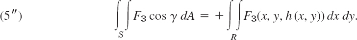
But if cos γ < 0, the integral on the right of (5″) gets a minus sign in front. This follows if we note that the element of area dx dy in the xy-plane is the projection |cos γ| dA of the element of area dA of S; and we have cos γ = +|cos γ| when cos γ > 0, but cos γ = −|cos γ| when cos γ < 0. Similarly for the other two terms in (5). At the same time, this justifies the notations in (5).
Other forms of surface integrals will be discussed later in this section.
EXAMPLE 1 Flux Through a Surface
Compute the flux of water through the parabolic cylinder S: y = x2, 0 ![]() x
x ![]() 2, 0
2, 0 ![]() z
z ![]() 3 (Fig. 245) if the velocity vector is v = F = [3z2, 6, 6xy], speed being measured in meters/sec. (Generally, F = ρv, but water has the density ρ = 1 g/cm3 = 1 ton/m3.)
3 (Fig. 245) if the velocity vector is v = F = [3z2, 6, 6xy], speed being measured in meters/sec. (Generally, F = ρv, but water has the density ρ = 1 g/cm3 = 1 ton/m3.)
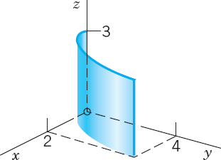
Fig. 245. Surface S in Example 1
Solution. Writing x = u and z = υ, we have y = x2 = u2. Hence a representation of S is
![]()
By differentiation and by the definition of the cross product,
![]()
On S, writing simply F(S) for F[r(u, υ)], we have F(S) = [3υ2, 6, 6uυ]. Hence F(S) • N = 6uυ2 − 6. By integration we thus get from (3) the flux
or 72,000 liters/sec. Note that the y-component of F is positive (equal to 6), so that in Fig. 245 the flow goes from left to right.
Let us confirm this result by (5). Since
![]()
we see that cos α > 0, cos β < 0, and cos γ. Hence the second term of (5) on the right gets a minus sign, and the last term is absent. This gives, in agreement with the previous result,

Evaluate (3) when F = [x2, 0, 3y2] and S is the portion of the plane x + y + z = 1 in the first octant (Fig. 246).
Solution. Writing x = u, and y = υ, we have z = 1 − x − y = 1 − u − υ. Hence we can represent the plane x + y + z = 1 in the form r(u, υ) = [u, υ, 1, − u − υ]. We obtain the first-octant portion S of this plane by restricting x = u and y = υ to the projection R of S in the xy-plane. R is the triangle bounded by the two coordinate axes and the straight line x + y = 1, obtained from x + y + z = 1 by setting z = 0. Thus 0 ![]() x
x ![]() 1 − y, 0
1 − y, 0 ![]() y
y ![]() 1.
1.
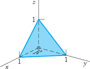
Fig. 246. Portion of a plane in Example 2
By inspection or by differentiation,
![]()
Hence F(S) • N = [u2, 0, 3υ2] • [1, 1, 1] = u2 + 3υ2. By (3),

Orientation of Surfaces
From (3) or (4) we see that the value of the integral depends on the choice of the unit normal vector n. (Instead of n we could choose −n.) We express this by saying that such an integral is an integral over an oriented surface S, that is, over a surface S on which we have chosen one of the two possible unit normal vectors in a continuous fashion. (For a piecewise smooth surface, this needs some further discussion, which we give below.) If we change the orientation of S, this means that we replace n with −n. Then each component of n in (4) is multiplied by −1 so that we have
THEOREM 1 Change of Orientation in a Surface Integral
The replacement of n by −n (hence of N by −N) corresponds to the multiplication of the integral in (3) or (4) by −1.
In practice, how do we make such a change of N happen, if S is given in the form (1)? The easiest way is to interchange u and υ, because then ru becomes rυ and conversely, so that N = ru × rυ becomes rυ × ru = −ru × rυ = −N, as wanted. Let us illustrate this.
EXAMPLE 3 Change of Orientation in a Surface Integral
In Example 1 we now represent S by ![]() , 0
, 0 ![]() υ
υ ![]() 2, 0
2, 0 ![]() u
u ![]() 3. Then
3. Then
![]()
For F = [3z2, 6, 6xz] we now get ![]() . Hence
. Hence ![]() and integration gives the old result times −1,
and integration gives the old result times −1,

Orientation of Smooth Surfaces
A smooth surface S (see Sec. 10.5) is called orientable if the positive normal direction, when given at an arbitrary point P0 of S, can be continued in a unique and continuous way to the entire surface. In many practical applications, the surfaces are smooth and thus orientable.
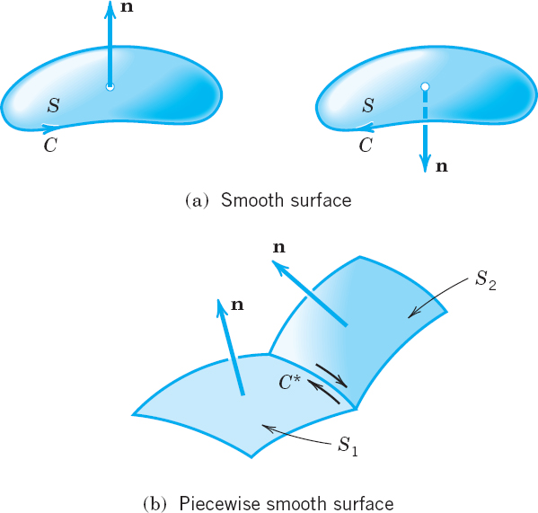
Fig. 247. Orientation of a surface
Orientation of Piecewise Smooth Surfaces
Here the following idea will do it. For a smooth orientable surface S with boundary curve C we may associate with each of the two possible orientations of S an orientation of C, as shown in Fig. 247a. Then a piecewise smooth surface is called orientable if we can orient each smooth piece of S so that along each curve C* which is a common boundary of two pieces S1 and S2 the positive direction of C* relative to S1 is opposite to the direction of C* relative to S2. See Fig. 247b for two adjacent pieces; note the arrows along C*.
Theory: Nonorientable Surfaces
A sufficiently small piece of a smooth surface is always orientable. This may not hold for entire surfaces. A well-known example is the Möbius strip,5 shown in Fig. 248. To make a model, take the rectangular paper in Fig. 248, make a half-twist, and join the short sides together so that A goes onto A, and B onto B. At P0 take a normal vector pointing, say, to the left. Displace it along C to the right (in the lower part of the figure) around the strip until you return to P0 and see that you get a normal vector pointing to the right, opposite to the given one. See also Prob. 17.

Surface Integrals Without Regard to Orientation
Another type of surface integral is
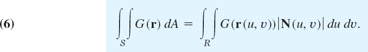
Here dA = |N| du dυ = |ru × rυ| du dυ is the element of area of the surface S represented by (1) and we disregard the orientation.
We shall need later (in Sec. 10.9) the mean value theorem for surface integrals, which states that if R in (6) is simply connected (see Sec. 10.2) and G(r) is continuous in a domain containing R, then there is a point (u0, υ0) in R such that

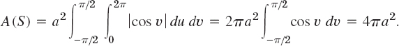
As for applications, if G(r) is the mass density of S, then (6) is the total mass of S. If G = 1, then (6) gives the area A(S) of S,

Examples 4 and 5 show how to apply (8) to a sphere and a torus. The final example, Example 6, explains how to calculate moments of inertia for a surface.
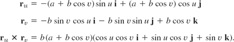
For a sphere r(u, υ) = [a cos υ cos u, a cos υ sin u, a sin υ], 0 ![]() u
u ![]() 2π, −π/2
2π, −π/2 ![]() u
u ![]() π/2 [see (3) in Sec. 10.5], we obtain by direct calculation (verify!)
π/2 [see (3) in Sec. 10.5], we obtain by direct calculation (verify!)
![]()
Using cos2 u + sin2 u = 1 and then cos2 υ + sin2 υ = 1, we obtain
![]()
With this, (8) gives the familiar formula (note that |cos υ| = cos υ when −π/2 ![]() υ
υ ![]() π/2)
π/2)
EXAMPLE 5 Torus Surface (Doughnut Surface): Representation and Area
A torus surface S is obtained by rotating a circle C about a straight line L in space so that C does not intersect or touch L but its plane always passes through L. If L is the z-axis and C has radius b and its center has distance a (> b) from L, as in Fig. 249, then S can be represented by
![]()
where 0 ![]() u
u ![]() 2π, 0
2π, 0 ![]() υ
υ ![]() 2π. Thus
2π. Thus
Hence |ru × rυ| = b(a × b cos υ), and (8) gives the total area of the torus,

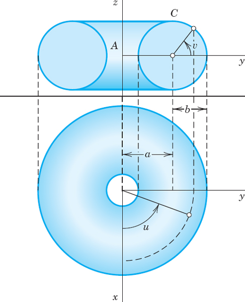
Fig. 249. Torus in Example 5
EXAMPLE 6 Moment of Inertia of a Surface
Find the moment of inertia I of a spherical lamina S: x2 + y2 + z2 = a2 of constant mass density and total mass M about the z-axis.
Solution. If a mass is distributed over a surface S and μ(x, y, z) is the density of the mass (= mass per unit area), then the moment of inertia I of the mass with respect to a given axis L is defined by the surface integral
where D(x, y, z) is the distance of the point (x, y, z) from L. Since, in the present example, μ is constant and S has the area A = 4πa2, we have μ = M/A = M/(4πa2).
For S we use the same representation as in Example 4. Then D2 = x2 + y2 = a2 cos2 υ. Also, as in that example, dA = a2 cos υ du dυ. This gives the following result. [In the integration, use cos3 υ = cos υ (1 − sin2 υ).]

Representations z = f(x, y). If a surface S is given by z = f(x, y), then setting u = x, υ = y, r = [u, υ, f] gives
![]()
and, since fu = fx, fυ = fy, formula (6) becomes
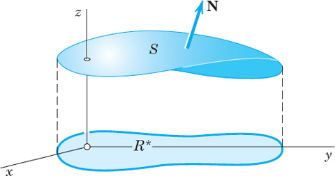
Here R* is the projection of S into the xy-plane (Fig. 250) and the normal vector N on S points up. If it points down, the integral on the right is preceded by a minus sign.
From (11) with G = 1 we obtain for the area A(S) of S: z = f(x, y) the formula

where R* is the projection of S into the xy-plane, as before.
1–10 FLUX INTEGRALS (3) ![]()
Evaluate the integral for the given data. Describe the kind of surface. Show the details of your work.
- F = [−x2, y2, 0], S: r = [u, υ, 3u − 2υ], 0 u 1.5, −2 υ 2
- F = [ey, ex, 1], S: x + y + z = 1, x 0, y 0, z 0
- F = [0, x, 0], S: x2 + y2 + z2 = 1, x 0, y 0, z 0
- F = [ey, −ez, ex], S: x2 + y2 = 25, x 0, y 0, 0 z 2
- F = [x, y, z], S: r = [u cos υ, u sin υ, u2], 0 u 4, −π υ π
- F = [cosh y, 0, sinh x], S; z = x + y2, 0 y x, 0 x 1
- F = [0, sin y, cos z], S the cylinder x = y2, where 0 y π/4 and 0 z y
- F = [tan xy, x, y], S: y2 + z2 = 1, 2 x 5, y 0, z 0
- F = [0, sinh z, cosh x], S: x2 + z2 = 4,
 , 0 y 5, z 0
 - F = [y2, x2, z4],
 , 0 z 8, y 0
 - CAS EXPERIMENT. Flux Integral. Write a program for evaluating surface integrals (3) that prints intermediate results (F, F • N, the integral over one of the two variables). Can you obtain experimentally some rules on functions and surfaces giving integrals that can be evaluated by the usual methods of calculus? Make a list of positive and negative results.
12–16 SURFACE INTEGRALS (6) ![]()
Evaluate these integrals for the following data. Indicate the kind of surface. Show the details.
- 12. G = cos x + sin x, S the portion of x + y + z = 1 in the first octant
- 13. G = x + y + z, z = x + 2y, 0 x π, 0 y x
- 14. G = ax + by + cz, S: x2 + y2 + z2 = 1, y = 0, z = 0
- 15. G = (1 + 9xz)3/2, S: r = [u, υ, u3], 0 u 1, −2 υ 2
- 16. G = arctan (y/x), S: z = x2 + y2, 1 z 9, x 0, y 0
- 17. Fun with Möbius. Make Möbius strips from long slim rectangles R of grid paper (graph paper) by pasting the short sides together after giving the paper a half-twist. In each case count the number of parts obtained by cutting along lines parallel to the edge. (a) Make R three squares wide and cut until you reach the beginning. (b) Make R four squares wide. Begin cutting one square away from the edge until you reach the beginning. Then cut the portion that is still two squares wide. (c) Make R five squares wide and cut similarly. (d) Make R six squares wide and cut. Formulate a conjecture about the number of parts obtained.
- 18. Gauss “Double Ring” (See Möbius, Works 2, 518–559). Make a paper cross (Fig. 251) into a “double ring” by joining opposite arms along their outer edges (without twist), one ring below the plane of the cross and the other above. Show experimentally that one can choose any four boundary points A, B, C, D and join A and C as well as B and D by two nonintersecting curves. What happens if you cut along the two curves? If you make a half-twist in each of the two rings and then cut? (Cf. E. Kreyszig, Proc. CSHPM 13 (2000), 23–43.)

APPLICATIONS
- 19. Center of gravity. Justify the following formulas for the mass M and the center of gravity
 of a lamina S of density (mass per unit area) σ(x, y, z) in space:

- 20. Moments of inertia. Justify the following formulas for the moments of inertia of the lamina in Prob. 19 about the x-, y-, and z-axes, respectively:
- 21. Find a formula for the moment of inertia of the lamina in Prob. 20 about the line y = x, z = 0.
22–23 Find the moment of inertia of a lamina S of density 1 about an axis B, where
- 22. S: x2 + y2 = 1, 0 z, h, B: the line z = h/2 in the xz- plane
- 23. S: x2 + y2 = z2, 0 z h, B: the z-axis
- 24. Steiner's theorem.6 If IB is the moment of inertia of a mass distribution of total mass M with respect to a line B through the center of gravity, show that its moment of inertia IK with respect to a line K, which is parallel to B and has the distance k from it is

- 25. Using Steiner's theorem, find the moment of inertia of a mass of density 1 on the sphere S: x2 + y2 + z2 = 1 about the line K: x = 1, y = 0 from the moment of inertia of the mass about a suitable line B, which you must first calculate.
- 26. TEAM PROJECT. First Fundamental Form ofS. Given a surface S: r(u, υ), the differential form

with coefficients (in standard notation, unrelated to F, G elsewhere in this chapter)

is called the first fundamental form of S. This form is basic because it permits us to calculate lengths, angles, and areas on S. To show this prove (a)–(c):
(a) For a curve C: u = u(t), υ = υ(t), a
t b, on S, formulas (10), Sec. 9.5, and (14) give the length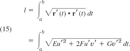
(b) The angle γ between two intersecting curves C1: u = g(t), υ = h(t) and C2: u = p(t), υ = q(t) on S: r(u, v) is obtained from

where a = rug′ + rυh′ and b = rup′ + rυq′ are tangent vectors of C1 and C2.
(c) The square of the length of the normal vector N can be written

so that formula (8) for the area A(S) of S becomes

(d) For polar coordinates u (= r) and υ (= θ) defined by x = u cos υ, y = u sin υ we have E = 1, F = 0, G = u2, so that

Calculate from this and (18) the area of a disk of radius a.
(e) Find the first fundamental form of the torus in Example 5. Use it to calculate the area A of the torus. Show that A can also be obtained by the theorem of Pappus,7 which states that the area of a surface of revolution equals the product of the length of a meridian C and the length of the path of the center of gravity of C when C is rotated through the angle 2π.
(f) Calculate the first fundamental form for the usual representations of important surfaces of your own choice (cylinder, cone, etc.) and apply them to the calculation of lengths and areas on these surfaces.
10.7 Triple Integrals. Divergence Theorem of Gauss
In this section we discuss another “big” integral theorem, the divergence theorem, which transforms surface integrals into triple integrals. So let us begin with a review of the latter.
A triple integral is an integral of a function f(x, y, z) taken over a closed bounded, three-dimensional region T in space. (Note that “closed” and “bounded” are defined in the same way as in footnote 2 of Sec. 10.3, with “sphere” substituted for “circle”). We subdivide T by planes parallel to the coordinate planes. Then we consider those boxes of the subdivision that lie entirely inside T, and number them from 1 to n. Here each box consists of a rectangular parallelepiped. In each such box we choose an arbitrary point, say, (xk, yk, zk) in box k. The volume of box k we denote by ΔVk. We now form the sum
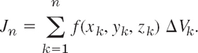
This we do for larger and larger positive integers n arbitrarily but so that the maximum length of all the edges of those n boxes approaches zero as n approaches infinity. This gives a sequence of real numbers ![]() . We assume that f(x, y, z) is continuous in a domain containing T, and T is bounded by finitely many smooth surfaces (see Sec. 10.5). Then it can be shown (see Ref. [GenRef4] in App. 1) that the sequence converges to a limit that is independent of the choice of subdivisions and corresponding points (xk, yk, zk). This limit is called the triple integralof f(x, y, z) over the region T and is denoted by
. We assume that f(x, y, z) is continuous in a domain containing T, and T is bounded by finitely many smooth surfaces (see Sec. 10.5). Then it can be shown (see Ref. [GenRef4] in App. 1) that the sequence converges to a limit that is independent of the choice of subdivisions and corresponding points (xk, yk, zk). This limit is called the triple integralof f(x, y, z) over the region T and is denoted by

Triple integrals can be evaluated by three successive integrations. This is similar to the evaluation of double integrals by two successive integrations, as discussed in Sec. 10.3. Example 1 below explains this.
Divergence Theorem of Gauss
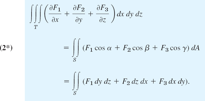
Triple integrals can be transformed into surface integrals over the boundary surface of a region in space and conversely. Such a transformation is of practical interest because one of the two kinds of integral is often simpler than the other. It also helps in establishing fundamental equations in fluid flow, heat conduction, etc., as we shall see. The transformation is done by the divergence theorem, which involves the divergence of a vector function F = [F1, F2, F3] = F1i + F2j + F3k, namely,

THEOREM 1 Divergence Theorem of Gauss (Transformation Between Triple and Surface Integrals)
Let T be a closed bounded region in space whose boundary is a piecewise smooth orientable surface S. Let F(x, y, z) be a vector function that is continuous and has continuous first partial derivatives in some domain containing T. Then

In components of F = [F1, F2, F3] and of the outer unit normal vector n = [cos α, cos β, cos γ] of S (as in Fig. 253), formula (2) becomes
“Closed bounded region” is explained above, “piecewise smooth orientable” in Sec. 10.5, and “domain containing T “in footnote 4, Sec. 10.4, for the two-dimensional case.
Before we prove the theorem, let us show a standard application.
EXAMPLE 1 Evaluation of a Surface Integral by the Divergence Theorem
Before we prove the theorem, let us show a typical application. Evaluate
where S is the closed surface in Fig. 252 consisting of the cylinder x2 + y2 = a2(0 ![]() z
z ![]() b) and the circular disks z = 0 and z = b(x2 + y2
b) and the circular disks z = 0 and z = b(x2 + y2 ![]() a2).
a2).
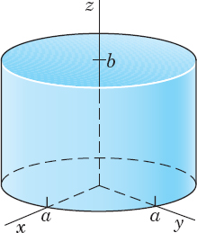
Fig. 252. Surface S in Example 1
Solution.. F1 = x3, F2 = x2y, F3 = x2z. Hence div F = 3x2 + x2 + x2 = 5x2. The form of the surface suggests that we introduce polar coordinates r, θ defined by x = r cos θ, y = r sin θ (thus cylindrical coordinates r, θ, z). Then the volume element is dx dy dz = r dr dθ dz, and we obtain

PROOF
We prove the divergence theorem, beginning with the first equation in (2*). This equation is true if and only if the integrals of each component on both sides are equal; that is,


We first prove (5) for a special regionT that is bounded by a piecewise smooth orientable surface S and has the property that any straight line parallel to any one of the coordinate axes and intersecting T has at most one segment (or a single point) in common with T. This implies that T can be represented in the form
![]()
where (x, y) varies in the orthogonal projection ![]() of T in the xy-plane. Clearly z = g(x, y), represents the “bottom” S2 of S (Fig. 253), whereas z = h(x, y) represents the “top” S1 of S, and there may be a remaining vertical portion S3 of S. (The portion S3 may degenerate into a curve, as for a sphere.)
of T in the xy-plane. Clearly z = g(x, y), represents the “bottom” S2 of S (Fig. 253), whereas z = h(x, y) represents the “top” S1 of S, and there may be a remaining vertical portion S3 of S. (The portion S3 may degenerate into a curve, as for a sphere.)
To prove (5), we use (6). Since F is continuously differentiable in some domain containing T, we have
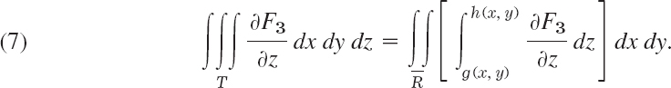
Integration of the inner integral […] gives F3[x, y, h(x, y)] − F3[x, y, g(x, y)]. Hence the triple integral in (7) equals


Fig. 253. Example of a special region
But the same result is also obtained by evaluating the right side of (5); that is [see also the last line of (2*)],
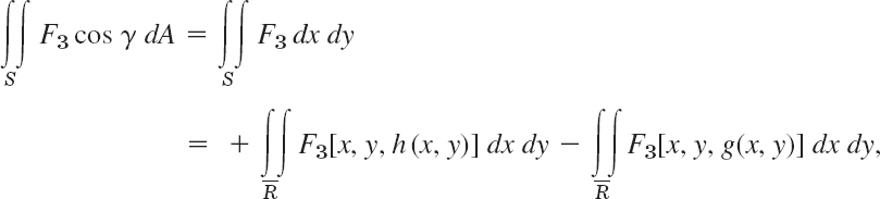
where the first integral over ![]() gets a plus sign because cos γ > 0 on S1 in Fig. 253 [as in (5″), Sec. 10.6], and the second integral gets a minus sign because cos γ < 0 on S2. This proves (5).
gets a plus sign because cos γ > 0 on S1 in Fig. 253 [as in (5″), Sec. 10.6], and the second integral gets a minus sign because cos γ < 0 on S2. This proves (5).
The relations (3) and (4) now follow by merely relabeling the variables and using the fact that, by assumption, T has representations similar to (6), namely,
![]()
This proves the first equation in (2*) for special regions. It implies (2) because the left side of (2*) is just the definition of the divergence, and the right sides of (2) and of the first equation in (2*) are equal, as was shown in the first line of (4) in the last section. Finally, equality of the right sides of (2) and (2*), last line, is seen from (5) in the last section.
This establishes the divergence theorem for special regions.
For any region T that can be subdivided into finitely many special regions by means of auxiliary surfaces, the theorem follows by adding the result for each part separately. This procedure is analogous to that in the proof of Green's theorem in Sec. 10.4. The surface integrals over the auxiliary surfaces cancel in pairs, and the sum of the remaining surface integrals is the surface integral over the whole boundary surface S of T; the triple integrals over the parts of T add up to the triple integral over T.
The divergence theorem is now proved for any bounded region that is of interest in practical problems. The extension to a most general region T of the type indicated in the theorem would require a certain limit process; this is similar to the situation in the case of Green's theorem in Sec. 10.4.
EXAMPLE 2 Verification of the Divergence Theorem
Evaluate ![]() over the sphere S: x2 + y2 + z2 = 4 (a) by (2), (b) directly.
over the sphere S: x2 + y2 + z2 = 4 (a) by (2), (b) directly.
Solution. (a) div F = div [7x, 0, −z] = div [7xi − zk] = 7 − 1 = 6. Answer:6 · ![]() .
.
(b) We can represent S by (3), Sec. 10.5 (with a = 2), and we shall use n dA = N du dυ [see (3*), Sec. 10.6]. Accordingly,
![]()
Then

Now on S we have x = 2 cos υ cos u, z = 2 sin υ, so that F = [7x, 0, −z] becomes on S
![]()
and

On S we have to integrate over u from 0 to 2π. This gives
![]()
The integral of cos υ sin2 υ equals (sin3 υ)/3, and that of cos3 υ = cos υ (1 − sin2 υ) equals sin υ − (sin3 υ)/3. On S we have −π/2 ![]() υ
υ ![]() π/2, so that by substituting these limits we get
π/2, so that by substituting these limits we get
![]()
as hoped for. To see the point of Gauss's theorem, compare the amounts of work.
Coordinate Invariance of the Divergence. The divergence (1) is defined in terms of coordinates, but we can use the divergence theorem to show that div F has a meaning independent of coordinates.
For this purpose we first note that triple integrals have properties quite similar to those of double integrals in Sec. 10.3. In particular, the mean value theorem for triple integrals asserts that for any continuous function f(x, y, z) in a bounded and simply connected region T there is a point Q: (x0, y0, z0) in T such that

In this formula we interchange the two sides, divide by V(T), and set f = div F. Then by the divergence theorem we obtain for the divergence an integral over the boundary surface S(T) of T,

We now choose a point P: (x1, y1, z1) in T and let T shrink down onto P so that the maximum distance d(T) of the points of T from P goes to zero. Then Q: (x0, y0, z0) must approach P. Hence (10) becomes
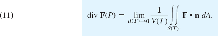
This proves
THEOREM 2 Invariance of the Divergence
The divergence of a vector function F with continuous first partial derivatives in a region T is independent of the particular choice of Cartesian coordinates. For any P in T it is given by (11).
Equation (11) is sometimes used as a definition of the divergence. Then the representation (1) in Cartesian coordinates can be derived from (11).
Further applications of the divergence theorem follow in the problem set and in the next section. The examples in the next section will also shed further light on the nature of the divergence.
1–8 APPLICATION: MASS DISTRIBUTION
Find the total mass of a mass distribution of density σ in a region T in space.
- σ = x2 + y2 + z2, T the box |x| 4, |y| 1, 0 z 2
- σ = xyz, T the box 0 x a, 0 y b, 0 z c
- σ = e−x−y−z, T: 0 x 1 − y, 0 y 1, 0 z 2
- σ as in Prob. 3, T the tetrahedron with vertices (0, 0, 0), (3, 0, 0), (0, 3, 0), (0, 0, 3)
- σ = sin 2x cos 2y,
 ,
,  , 0 z 6
 - σ x2y2z2, T the cylindrical region x2 + z2 16, |y| 4
- σ = arctan (y/x), T: x2 + y2 + z2 a2, z 0
- σ = x2 + y2, T as in Prob. 7
9–18 APPLICATION OF THE DIVERGENCE THEOREM
Evaluate the surface integral ![]() by the divergence theorem. Show the details.
by the divergence theorem. Show the details.
- 9. F = [x2, 0, z2], S the surface of the box |x| 1, |y| 3, 0 z 2
- 10. Solve Prob. 9 by direct integration.
- 11. F = [ex, ey, ez], S the surface of the cube |x| 1, |y| 1, |z| 1
- 12. F = [x3 − y3, y3 − z3, z3 − x3], S the surface of x2 + y2 + z2 25, z 0
- 13. F = [sin y, cos x, cos z], S, the surface of x2 + y2 4, |z| 2 (a cylinder and two disks!)
- 14. F as in Prob. 13, S the surface of x2 + y2 9, 0 z 2
- 15.
 , S the surface of the tetrahedron with vertices (0, 0, 0), (1, 0, 0), (0, 1, 0), (0, 0, 1)
 - 16. F = [cosh x, z, y], S as in Prob. 15
- 17. F = [x2, y2, z2], S the surface of the cone x2 + y2 z2, 0 z h
- 18. F = [xy, yz, zx], S the surface of the cone x2 + y2 4z2, 0 z 2
19–23 APPLICATION: MOMENT OF INERTIA
Given a mass of density 1 in a region T of space, find the moment of intertia about the x-axis
- 19. The box −a x a, −b y b, −c z c
- 20. The ball x2 + y2 + z2 a2
- 21. The cylinder y2 + z2 a2, 0 x h
- 22. The paraboloid y2 + z2 x, 0 x h
- 23. The cone y2 + z2 x2, 0 x h
- 24. Why is Ix in Prob. 23 for large h larger than Ix in Prob. 22 (and the same h)? Why is it smaller for h = 1? Give physical reason.
- 25. Show that for a solid of revolution,
 . Solve Probs. 20–23 by this formula.
10.8 Further Applications of the Divergence Theorem
The divergence theorem has many important applications: In fluid flow, it helps characterize sources and sinks of fluids. In heat flow, it leads to the heat equation. In potential theory, it gives properties of the solutions of Laplace's equation. In this section, we assume that the region T and its boundary surface S are such that the divergence theorem applies.
EXAMPLE 1 Fluid Flow. Physical Interpretation of the Divergence
From the divergence theorem we may obtain an intuitive interpretation of the divergence of a vector. For this purpose we consider the flow of an incompressible fluid (see Sec. 9.8) of constant density ρ = 1 which is steady, that is, does not vary with time. Such a flow is determined by the field of its velocity vector v(P) at any point P.
Let S be the boundary surface of a region T in space, and let n be the outer unit normal vector of S. Then v • n is the normal component of v in the direction of n, and |v • n dA| is the mass of fluid leaving T (if v • n > 0 at some P) or entering T (if v • n ≤ 0 at P) per unit time at some point P of S through a small portion ΔS of S area ΔA. Hence the total mass of fluid that flows across S from T to the outside per unit time is given by the surface integral

Division by the volume V of T gives the average flow out of T:

Since the flow is steady and the fluid is incompressible, the amount of fluid flowing outward must be continuously supplied. Hence, if the value of the integral (1) is different from zero, there must be sources (positive sources and negative sources, called sinks) in T, that is, points where fluid is produced or disappears.
If we let T shrink down to a fixed point P in T, we obtain from (1) the source intensity at P given by the right side of (11) in the last section with F • n replaced by v • n, that is,
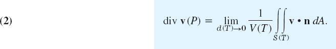
Hence the divergence of the velocity vector v of a steady incompressible flow is the source intensity of the flow at the corresponding point.
There are no sources in T if and only if div v is zero everywhere in T. Then for any closed surface S in T we have

EXAMPLE 2 Modeling of Heat Flow. Heat or Diffusion Equation
Physical experiments show that in a body, heat flows in the direction of decreasing temperature, and the rate of flow is proportional to the gradient of the temperature. This means that the velocity v of the heat flow in a body is of the form
![]()
where U(x, y, z, t) is temperature, t is time, and K is called the thermal conductivity of the body; in ordinary physical circumstances K is a constant. Using this information, set up the mathematical model of heat flow, the so-called heat equation or diffusion equation.
Solution. Let T be a region in the body bounded by a surface S with outer unit normal vector n such that the divergence theorem applies. Then v · n is the component of v in the direction of n, and the amount of heat leaving T per unit time is

This expression is obtained similarly to the corresponding surface integral in the last example. Using
![]()
(the Laplacian; see (3) in Sec. 9.8), we have by the divergence theorem and (3)
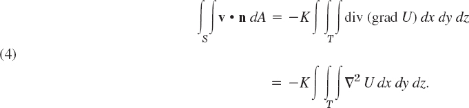
On the other hand, the total amount of heat H in T is
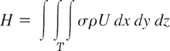
where the constant σ is the specific heat of the material of the body and ρ is the density (= mass per unit volume) of the material. Hence the time rate of decrease of H is
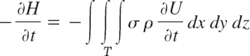
and this must be equal to the above amount of heat leaving T. From (4) we thus have
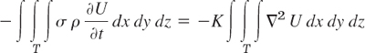
or

Since this holds for any region T in the body, the integrand (if continuous) must be zero everywhere; that is,

where c2 is called the thermal diffusivity of the material. This partial differential equation is called the heat equation. It is the fundamental equation for heat conduction. And our derivation is another impressive demonstration of the great importance of the divergence theorem. Methods for solving heat problems will be shown in Chap. 12.
The heat equation is also called the diffusion equation because it also models diffusion processes of motions of molecules tending to level off differences in density or pressure in gases or liquids.
If heat flow does not depend on time, it is called steady-state heat flow. Then ∂U/∂t = 0, so that (5) reduces to Laplace's equation ∇2U = 0. We met this equation in Secs. 9.7 and 9.8, and we shall now see that the divergence theorem adds basic insights into the nature of solutions of this equation.
Potential Theory. Harmonic Functions
The theory of solutions of Laplace's equation
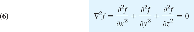
is called potential theory. A solution of (6) with continuous second-order partial derivatives is called a harmonic function. That continuity is needed for application of the divergence theorem in potential theory, where the theorem plays a key role that we want to explore. Further details of potential theory follow in Chaps. 12 and 18.
EXAMPLE 3 A Basic Property of Solutions of Laplace's Equation
The integrands in the divergence theorem are div F and F • n (Sec. 10.7). If F is the gradient of a scalar function, say, F = grad f, then div F = div (grad f) = ∇2f; see (3), Sec. 9.8. Also, F • n = n • F = n • grad f. This is the directional derivative of f in the outer normal direction of S, the boundary surface of the region T in the theorem. This derivative is called the (outer) normal derivative of f and is denoted by ∂f/∂n. Thus the formula in the divergence theorem becomes
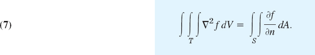
This is the three-dimensional analog of (9) in Sec. 10.4. Because of the assumptions in the divergence theorem this gives the following result.
THEOREM 1 A Basic Property of Harmonic Functions
Let f(x, y, z) be a harmonic function in some domain D is space. Let S be any piecewise smooth closed orientable surface in D whose entire region it encloses belongs to D. Then the integral of the normal derivative of f taken over S is zero. (For “piecewise smooth” see Sec. 10.5.)
Let f and g be scalar functions such that F = f grad g satisfies the assumptions of the divergence theorem in some region T. Then

Also, since f is a scalar function,
Now n • grad g is the directional derivative ∂g/∂n of g in the outer normal direction of S. Hence the formula in the divergence theorem becomes “Green's first formula”

Formula (8) together with the assumptions is known as the first form of Green's theorem.
Interchanging f and g we obtain a similar formula. Subtracting this formula from (8) we find

This formula is called Green's second formula or (together with the assumptions) the second form of Green's theorem.
EXAMPLE 5 Uniqueness of Solutions of Laplace's Equation
Let f be harmonic in a domain D and let f be zero everywhere on a piecewise smooth closed orientable surface S in D whose entire region T it encloses belongs to D. Then ∇2g is zero in T, and the surface integral in (8) is zero, so that (8) with g = f gives
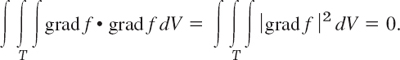
Since f is harmonic, grad f and thus |grad f| are continuous in T and on S, and since |grad f| is nonnegative, to make the integral over T zero, grad f must be the zero vector everywhere in T. Hence fx = fy = fz = 0, and f is constant in T and, because of continuity, it is equal to its value 0 on S. This proves the following theorem.
Let f(x, y, z) be harmonic in some domain D and zero at every point of a piecewise smooth closed orientable surface S in D whose entire region T it encloses belongs to D. Then f is identically zero in T.
This theorem has an important consequence. Let f1 and f2 be functions that satisfy the assumptions of Theorem 1 and take on the same values on S. Then their difference f1 − f2 satisfies those assumptions and has the value 0 everywhere on S. Hence, Theorem 2 implies that
![]()
and we have the following fundamental result.
THEOREM 3 Uniqueness Theorem for Laplace's Equation
Let T be a region that satisfies the assumptions of the divergence theorem, and let f(x, y, z) be a harmonic function in a domain D that contains T and its boundary surface S. Then f is uniquely determined in T by its values on S.
The problem of determining a solution u of a partial differential equation in a region T such that u assumes given values on the boundary surface S of T is called the Dirichlet problem.8 We may thus reformulate Theorem 3 as follows.
THEOREM 3* Uniqueness Theorem for the Dirichlet Problem
If the assumptions in Theorem 3 are satisfied and the Dirichlet problem for the Laplace equation has a solution in T, then this solution is unique.
These theorems demonstrate the extreme importance of the divergence theorem in potential theory.
1–6 VERIFICATIONS
- Harmonic functions. Verify Theorem 1 for f = 2z2 − x2 − y2 and S the surface of the box 0 x a, 0 y b, 0 z c.
- Harmonic functions. Verify Theorem 1 for f = x2 − y2 and the surface of the cylinder x2 + y2 = 4, 0 z h.
- Green's first identity. Verify (8) for f = 4y2, g = x2, S the surface of the “unit cube” 0 x 1, 0 y 1, 0 z 1. What are the assumptions on f and g in (8)? Must f and g be harmonic?
- Green's first identity. Verify (8) for f = x, g = y2 + z2, S the surface of the box 0 x 1, 0 y 2, 0 z 3.
- Green's second identity. Verify (9) for f = 6y2, g = 2x2, S the unit cube in Prob. 3.
- Green's second identity. Verify (9) for f = x2, g = y4, S the unit cube in Prob. 3.
7–11 VOLUME
Use the divergence theorem, assuming that the assumptions on T and S are satisfied.
- 7. Show that a region T with boundary surface S has the volume

- 8. Cone. Using the third expression for υ in Prob. 7, verify V = πa2 h/3 for the volume of a circular cone of height h and radius of base a.
- 9. Ball. Find the volume under a hemisphere of radius a from in Prob. 7.
- 10. Volume. Show that a region T with boundary surface S has the volume

where r is the distance of a variable point P: (x, y, z) on S from the origin O and φ is the angle between the directed line OP and the outer normal of S at P. Make a sketch. Hint. Use (2) in Sec. 10.7 with F = [x, y, z].
- 11. Ball. Find the volume of a ball of radius a from Prob. 10.
- 12. TEAM PROJECT. Divergence Theorem and Potential Theory. The importance of the divergence theorem in potential theory is obvious from (7)–(9) and Theorems 1–3. To emphasize it further, consider functions f and g that are harmonic in some domain D containing a region T with boundary surface S such that T satisfies the assumptions in the divergence theorem. Prove, and illustrate by examples, that then:
(a)

(b) If ∂g/∂n = 0 on S, then g is constant in T.
(c)

(d) If ∂f/∂n = ∂g/∂n on S, then f = g + c in T, where c is a constant.
(e) The Laplacian can be represented independently of coordinate systems in the form

where d(T) is the maximum distance of the points of a region T bounded by S(T) from the point at which the Laplacian is evaluated and V(T) is the volume of T.
10.9 Stokes's Theorem
Let us review some of the material covered so far. Double integrals over a region in the plane can be transformed into line integrals over the boundary curve of that region and conversely, line integrals into double integrals. This important result is known as Green's theorem in the plane and was explained in Sec. 10.4. We also learned that we can transform triple integrals into surface integrals and vice versa, that is, surface integrals into triple integrals. This “big” theorem is called Gauss's divergence theorem and was shown in Sec. 10.7.
To complete our discussion on transforming integrals, we now introduce another “big” theorem that allows us to transform surface integrals into line integrals and conversely, line integrals into surface integrals. It is called Stokes's Theorem, and it generalizes Green's theorem in the plane (see Example 2 below for this immediate observation). Recall from Sec. 9.9 that
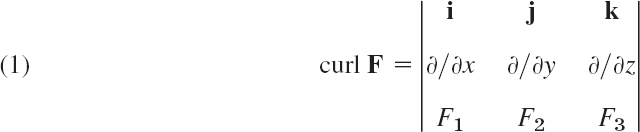
which we will need immediately.
THEOREM 1 Stokes's Theorem9 (Transformation Between Surface and Line Integrals)
Let S be a piecewise smooth9 oriented surface in space and let the boundary of S be a piecewise smooth simple closed curve C. Let F(x, y, z) be a continuous vector function that has continuous first partial derivatives in a domain in space containing S. Then

Here n is a unit normal vector of S and, depending on n, the integration around C is taken in the sense shown in Fig. 254. Furthermore, r′ = dr/ds is the unit tangent vector and s the arc length of C.
In components, formula (2) becomes
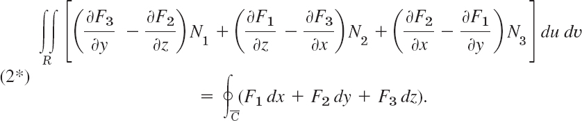
Here,, F = [F1, F2, F3], N = [N1, N2, N3], n dA = N du dυ, r′ ds = [dx, dy, dz], and R is the region with boundary curve ![]() in the uυ-plane corresponding to S represented by r(u, υ).
in the uυ-plane corresponding to S represented by r(u, υ).
The proof follows after Example 1.

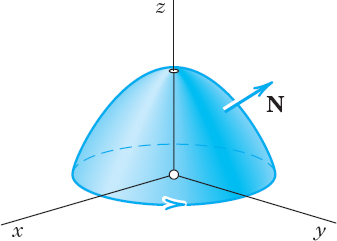
Fig. 255. Surface S in Example 1
EXAMPLE 1 Verification of Stokes's Theorem
Before we prove Stokes's theorem, let us first get used to it by verifying it for F = [y, z, x] and S the paraboloid (Fig. 255)
![]()
Solution. The curve C, oriented as in Fig. 255, is the circle r(s) = [cos s, sin s, 0]. Its unit tangent vector is r′(s) = [−sin s, cos s, 0]. The function F = [y, z, x] on C is F (r(s)) = [sin s, 0, cos s]. Hence
![]()
We now consider the surface integral. We have F1 = y, F2 = z, F3 = x, so that in (2*) we obtain
![]()
A normal vector of S is N = grad (z − f(x, y)) = [2x, 2y, 1]. Hence (curl F) • N = −2x − 2y − 1. Now n dA = N dx dy (see (3*) in Sec. 10.6 with x, y instead of u, υ). Using polar coordinates r, θ defined by x = r cos θ, y = r sin θ and denoting the projection of S into the xy-plane by R, we thus obtain

PROOF
We prove Stokes's theorem. Obviously, (2) holds if the integrals of each component on both sides of (2*) are equal; that is,
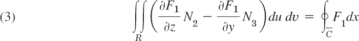

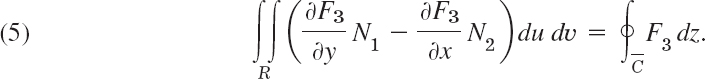
We prove this first for a surface S that can be represented simultaneously in the forms
![]()
We prove (3), using (6a). Setting u = x, υ = y, we have from (6a)
![]()
and in (2), Sec. 10.6, by direct calculation
![]()
Note that N is an upper normal vector of S, since it has a positive z-component. Also, R = S*, the projection of S into the xy-plane, with boundary curve ![]() (Fig. 256). Hence the left side of (3) is
(Fig. 256). Hence the left side of (3) is
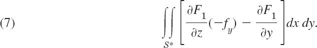
We now consider the right side of (3). We transform this line integral over ![]() into a double integral over S* by applying Green's theorem [formula (1) in Sec. 10.4 with F2 = 0]. This gives
into a double integral over S* by applying Green's theorem [formula (1) in Sec. 10.4 with F2 = 0]. This gives


Fig. 256. Proof of Stokes's theorem
Here, F1 = F1(x, y, f(x, y)). Hence by the chain rule (see also Prob. 10 in Problem Set 9.6),

We see that the right side of this equals the integrand in (7). This proves (3). Relations (4) and (5) follow in the same way if we use (6b) and (6c), respectively. By addition we obtain (2*). This proves Stokes's theorem for a surface S that can be represented simultaneously in the forms (6a), (6b), (6c).
As in the proof of the divergence theorem, our result may be immediately extended to a surface S that can be decomposed into finitely many pieces, each of which is of the kind just considered. This covers most of the cases of practical interest. The proof in the case of a most general surface S satisfying the assumptions of the theorem would require a limit process; this is similar to the situation in the case of Green's theorem in Sec. 10.4.
EXAMPLE 2 Green's Theorem in the Plane as a Special Case of Stokes's Theorem
Let F = [F1, F2] = F1i + F2j be a vector function that is continuously differentiable in a domain in the xy-plane containing a simply connected bounded closed region S whose boundary C is a piecewise smooth simple closed curve. Then, according to (1),

Hence the formula in Stokes's theorem now takes the form
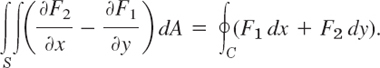
This shows that Green's theorem in the plane (Sec. 10.4) is a special case of Stokes's theorem (which we needed in the proof of the latter!).
EXAMPLE 3 Evaluation of a Line Integral by Stokes's Theorem
Evaluate ∫C F • r′ ds, where C is the circle x2 + y2 = 4, z = −3, oriented counterclockwise as seen by a person standing at the origin, and, with respect to right-handed Cartesian coordinates,
![]()
Solution. As a surface S bounded by C we can take the plane circular disk x2 + y2 ![]() 4 in the plane z = −3. Then n in Stokes's theorem points in the positive z-direction; thus n = k. Hence (curl F) • n is simply the component of curl F in the positive z-direction. Since F with z = −3 has the components F1 = y, F2 = −27x, F3 = 3y3, we thus obtain
4 in the plane z = −3. Then n in Stokes's theorem points in the positive z-direction; thus n = k. Hence (curl F) • n is simply the component of curl F in the positive z-direction. Since F with z = −3 has the components F1 = y, F2 = −27x, F3 = 3y3, we thus obtain

Hence the integral over S in Stokes's theorem equals −28 times the area 4π of the disk S. This yields the answer −28 · 4π = −112π ≈ −352. Confirm this by direct calculation, which involves somewhat more work.
EXAMPLE 4 Physical Meaning of the Curl in Fluid Motion. Circulation
Let Sro be a circular disk of radius r0 and center P bounded by the circle Cr0 (Fig. 257), and let F(Q) ≡ F(x, y, z) be a continuously differentiable vector function in a domain containing Sr0. Then by Stokes's theorem and the mean value theorem for surface integrals (see Sec. 10.6),

where Ar0 is the area of Sr0 and P* is a suitable point of Sr0. This may be written in the form
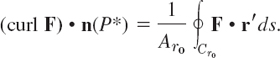
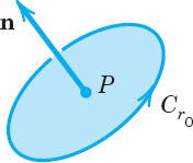
Fig. 257. Example 4
In the case of a fluid motion with velocity vector F = v, the integral

is called the circulation of the flow around Cr0. It measures the extent to which the corresponding fluid motion is a rotation around the circle Cr0. If we now let r0 approach zero, we find

that is, the component of the curl in the positive normal direction can be regarded as the specific circulation (circulation per unit area) of the flow in the surface at the corresponding point.
EXAMPLE 5 Work Done in the Displacement around a Closed Curve
Find the work done by the force F = 2xy3 sin zi + 3x2y2 sin zj + x2y3 cos z k in the displacement around the curve of intersection of the paraboloid z = x2 + y2 and the cylinder (x − 1)2 + y2 = 1.
Solution. This work is given by the line integral in Stokes's theorem. Now F = grad f, where f = x2y3 sin z and curl (grad f) = 0 (see (2) in Sec. 9.9), so that (curl F) • n = 0 and the work is 0 by Stokes's theorem. This agrees with the fact that the present field is conservative (definition in Sec. 9.7).
Stokes's Theorem Applied to Path Independence
We emphasized in Sec. 10.2 that the value of a line integral generally depends not only on the function to be integrated and on the two endpoints A and B of the path of integration C, but also on the particular choice of a path from A to B. In Theorem 3 of Sec. 10.2 we proved that if a line integral
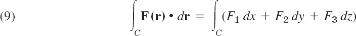
(involving continuous F1, F2, F3 that have continuous first partial derivatives) is path independent in a domain D, then curl F = 0 in D. And we claimed in Sec. 10.2 that, conversely, curl F = 0 everywhere in D implies path independence of (9) in D provided D is simply connected. A proof of this needs Stokes's theorem and can now be given as follows.
Let C be any closed path in D. Since D is simply connected, we can find a surface S in D bounded by C. Stokes's theorem applies and gives

for proper direction on C and normal vector n on S. Since curl F = 0 in D, the surface integral and hence the line integral are zero. This and Theorem 2 of Sec. 10.2 imply that the integral (9) is path independent in D. This completes the proof.
1–10 DIRECT INTEGRATION OF SURFACE INTEGRALS
Evaluate the surface integral ![]() directly for the given F and S.
directly for the given F and S.
- F = [z2, −x2, 0], S the rectangle with vertices (0, 0, 0), (1, 0, 0), (0, 4, 4), (1, 4, 4)
- F = [−13 sin y, 3 sinh z, x], S the rectangle with vertices (0, 0, 2), (4, 0, 2), (4, π/2, 2), (0, π/2, 2)
- F = [e−z, e−z cos y, e−z sin y], S: z = y2/2, −1 x 1, 0 y 1
- F as in Prob. 1, z = xy (0 x 1, 0 y 4). Compare with Prob. 1.
 , S: 0 x a, 0 y a, z = 1
- F = [y3, −x3, 0], S: x2 + y2 1, z = 0
- F = [ey, ez, ex], S: z = x2 (0 x 2, 0 y 1)
- F = [z2, x2, y2],
 , y 0, 0 z h
 - Verify Stokes's theorem for F and S in Prob. 5.
- Verify Stokes's theorem for F and S in Prob. 6.
- Stokes's theorem not applicable. Evaluate
 , F = (x2 + y2)−1 [−y, x], C: x2 + y2 = 1, z = 0, oriented clockwise. Why can Stokes's theorem not be applied? What (false) result would it give?
 - WRITING PROJECT. Grad, Div, Curl in Connection with Integrals. Make a list of ideas and results on this topic in this chapter. See whether you can rearrange or combine parts of your material. Then subdivide the material into 3–5 portions and work out the details of each portion. Include no proofs but simple typical examples of your own that lead to a better understanding of the material.
13–20 EVALUATION OF ![]()
Calculate this line integral by Stokes's theorem for the given F and C. Assume the Cartesian coordinates to be right-handed and the z-component of the surface normal to be nonnegative.
- 13. F = [−5y, 4x, z], C the circle x2 + y2 = 16, z = 4
- 14. F = [z3, x3, y3], C the circle x = 2, y2 + z2 = 9
- 15. F = [y2, x2, z + x] around the triangle with vertices (0, 0, 0), (1, 0, 0), (1, 1, 0)
- 16. F = [ey, 0, ex], C as in Prob. 15
- 17. F = [0, z3, 0], C the boundary curve of the cylinder x2 + y2 = 1, x 0, y 0, 0 z 1
- 18. F = [−y, 2z, 0], C the boundary curve of y2 + z2 = 4, z 0, 0 x h
- 19. F = [z, ez, 0], C the boundary curve of the portion of the cone
 , x 0, y 0, 0 z 1
 - 20. F = [0, cos x, 0], C the boundary curve of y2 + z2 = 4, y 0, z 0, 0 x π
CHAPTER 10 REVIEW QUESTIONS AND PROBLEMS
- State from memory how to evaluate a line integral. A surface integral.
- What is path independence of a line integral? What is its physical meaning and importance?
- What line integrals can be converted to surface integrals and conversely? How?
- What surface integrals can be converted to volume integrals? How?
- What role did the gradient play in this chapter? The curl? State the definitions from memory.
- What are typical applications of line integrals? Of surface integrals?
- Where did orientation of a surface play a role? Explain.
- State the divergence theorem from memory. Give applications.
- In some line and surface integrals we started from vector functions, but integrands were scalar functions. How and why did we proceed in this way?
- State Laplace's equation. Explain its physical importance. Summarize our discussion on harmonic functions.
11–20 LINE INTEGRALS (WORK INTEGRALS)
Evaluate ![]() for given F and C by the method that seems most suitable. Remember that if F is a force, the integral gives the work done in the displacement along C. Show details.
for given F and C by the method that seems most suitable. Remember that if F is a force, the integral gives the work done in the displacement along C. Show details.
- 11. F = [2x2, −4y2], C the straight-line segment from to (4, 2) to (−6, 10)
- 12. F = [y cos xy, x cos xy, ez], C the straight-line segment from (π, 1, 0) to

- 13. F = [y2, 2xy + 5 sin x, 0], C the boundary of 0 x π/2, 0 y 2, z = 0
- 14. F = [−y3, x3 + e−y, 0], C the circle x2 + y2 = 25, z = 2
- 15. F = [x3, e2y, e−4z], C: x2 + 9y2 = 9, z = x2
- 16. F = [x2, y2, y2x], C the helix r = [2 cos t, 2 sin t, 3t] from to (2, 0, 0) to (−2, 0, 3π)
- 17. F = [9z, 5x, 3y], C the ellipse x2 + y2 = 9, z = x + 2
- 18. F = [sin πy, cos πx, sin πx], C the boundary curve of 0 x 1, 0 y 2, z = x
- 19. F = [z, 2y, x], C the helix r [cos t, sin t, t] from (1, 0, 0) to (1, 0, 2π)
- 20. F = [zexz, 2 sinh 2y, xexz], C the parabola y = x, z = x2, −1 x 1
21–25 DOUBLE INTEGRALS, CENTER OF GRAVITY
Find the coordinates ![]() of the center of gravity of a mass of density f(x, y) in the region R. Sketch R, show details.
of the center of gravity of a mass of density f(x, y) in the region R. Sketch R, show details.
- 21. f = xy, R the triangle with vertices (0, 0), (2, 0), (2, 2)
- 22. f = x2 + y2, R: x2 + y2 a2, y 0
- 23. f = x2, R: −1 x 2, x2 y x + 2. Why is
 ?
? - 24. f = 1, R: 0 y 1 − x4
- 25. f = ky, k > 0, arbitrary, 0 y 1 − x2, 0 x 1
- 26. Why are
 and
and  in Prob. 25 independent of k?
27–35 SURFACE INTEGRALS ![]() DIVERGENCE THEOREM
DIVERGENCE THEOREM
Evaluate the integral diectly or, if possible, by the divergence theorem. Show details.
- 27. F = [ax, by, cz], S the sphere x2 + y2 + z2 = 36
- 28. F = [x + y2, y + z2, z + x2], S the ellipsoid with semi-axes of lengths a, b, c
- 29. F = [y + z, 20y, 2z3], S the surface of 0 x 2, 0 y 1, 0 z y
- 30. F = [1, 1, 1], S: x2 + y2 + 4z2 = 4, z 0
- 31. F = [ex, ey, ez], S the surface of the box |x| 1, |y| 1, |z| 1
- 32. F = [y2, x2, z2], S the portion of the paraboloid z = x2 + y2, z 9
- 33. F = [y2, x2, z2], S: r = [u, u2, υ], 0 u 2, −2 υ 2
- 34. F = [x, xy, z], S the boundary of x2 + y2 1, 0 z 5
- 35. F = [x + z, y + z, x + y], S the sphere of radius 3 with center 0
SUMMARY OF CHAPTER 10 Vector Integral Calculus. Integral Theorems
Chapter 9 extended differential calculus to vectors, that is, to vector functions v(x, y, z) or v(t). Similarly, Chapter 10 extends integral calculus to vector functions. This involves line integrals (Sec. 10.1), double integrals (Sec. 10.3), surface integrals (Sec. 10.6), and triple integrals (Sec. 10.7) and the three “big” theorems for transforming these integrals into one another, the theorems of Green (Sec. 10.4), Gauss (Sec. 10.7), and Stokes (Sec. 10.9).
The analog of the definite integral of calculus is the line integral (Sec. 10.1)

where C: r(t) = [x(t), y(t), z(t)] = x(t)i + y(t)j + z(t)k (a ![]() t
t ![]() b) is a curve in space (or in the plane). Physically, (1) may represent the work done by a (variable) force in a displacement. Other kinds of line integrals and their applications are also discussed in Sec. 10.1.
b) is a curve in space (or in the plane). Physically, (1) may represent the work done by a (variable) force in a displacement. Other kinds of line integrals and their applications are also discussed in Sec. 10.1.
Independence of path of a line integral in a domain D means that the integral of a given function over any path C with endpoints P and Q has the same value for all paths from P to Q that lie in D; here P and Q are fixed. An integral (1) is independent of path in D if and only if the differential form F1 dx + F2 dy + F3 dz with continuous F1, F2, F3 is exact in D (Sec. 10.2). Also, if curl F = 0, where F = [F1, F2, F3], has continuous first partial derivatives in a simply connected domain D, then the integral (1) is independent of path in D (Sec. 10.2).
Integral Theorems. The formula of Green's theorem in the plane (Sec. 10.4)

transforms double integrals over a region R in the xy-plane into line integrals over the boundary curve C of R and conversely. For other forms of (2) see Sec. 10.4.
Similarly, the formula of the divergence theorem of Gauss (Sec. 10.7)

transforms triple integrals over a region T in space into surface integrals over the boundary surface S of T, and conversely. Formula (3) implies Green's formulas
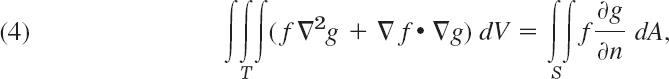

Finally, the formula of Stokes's theorem (Sec. 10.9)
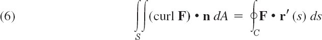
transforms surface integrals over a surface S into line integrals over the boundary curve C of S and conversely.
1 JOHANN FRIEDRICH PFAFF (1765–1825). German mathematician.
2 A region R is a domain (Sec. 9.6) plus, perhaps, some or all of its boundary points. R is closed if its boundary (all its boundary points) are regarded as belonging to R; and R is bounded if it can be enclosed in a circle of sufficiently large radius. A boundary point P of R is a point (of R or not) such that every disk with center P contains points of R and also points not of R.
3 Named after the German mathematician CARL GUSTAV JACOB JACOBI (1804–1851), known for his contributions to elliptic functions, partial differential equations, and mechanics.
4 GEORGE GREEN (1793–1841), English mathematician who was self-educated, started out as a baker, and at his death was fellow of Caius College, Cambridge. His work concerned potential theory in connection with electricity and magnetism, vibrations, waves, and elasticity theory. It remained almost unknown, even in England, until after his death.
A “domain containing R” in the theorem guarantees that the assumptions about F1 and F2 at boundary points of R are the same as at other points of R.
5 AUGUST FERDINAND MÖBIUS (1790–1868), German mathematician, student of Gauss, known for his work in surface theory, geometry, and complex analysis (see Sec. 17.2).
6 JACOB STEINER (1796–1863), Swiss geometer, born in a small village, learned to write only at age 14, became a pupil of Pestalozzi at 18, later studied at Heidelberg and Berlin and, finally, because of his outstanding research, was appointed professor at Berlin University.
7 PAPPUS OF ALEXANDRIA (about A.D. 300), Greek mathematician. The theorem is also called Guldin's theorem. HABAKUK GULDIN (1577–1643) was born in St. Gallen, Switzerland, and later became professor in Graz and Vienna.
8 PETER GUSTAV LEJEUNE DIRICHLET (1805–1859), German mathematician, studied in Paris under Cauchy and others and succeeded Gauss at Göttingen in 1855. He became known by his important research on Fourier series (he knew Fourier personally) and in number theory.
9 Sir GEORGE GABRIEL STOKES (1819–1903), Irish mathematician and physicist who became a professor in Cambridge in 1849. He is also known for his important contribution to the theory of infinite series and to viscous flow (Navier–Stokes equations), geodesy, and optics.
“Piecewise smooth” curves and surfaces are defined in Secs. 10.1 and 10.5.