
CHAPTER 12
Partial Differential Equations (PDEs)
A PDE is an equation that contains one or more partial derivatives of an unknown function that depends on at least two variables. Usually one of these deals with time t and the remaining with space (spatial variable(s)). The most important PDEs are the wave equations that can model the vibrating string (Secs. 12.2, 12.3, 12.4, 12.12) and the vibrating membrane (Secs. 12.8, 12.9, 12.10), the heat equation for temperature in a bar or wire (Secs. 12.5, 12.6), and the Laplace equation for electrostatic potentials (Secs. 12.6, 12.10, 12.11). PDEs are very important in dynamics, elasticity, heat transfer, electromagnetic theory, and quantum mechanics. They have a much wider range of applications than ODEs, which can model only the simplest physical systems. Thus PDEs are subjects of many ongoing research and development projects.
Realizing that modeling with PDEs is more involved than modeling with ODEs, we take a gradual, well-planned approach to modeling with PDEs. To do this we carefully derive the PDE that models the phenomena, such as the one-dimensional wave equation for a vibrating elastic string (say a violin string) in Sec. 12.2, and then solve the PDE in a separate section, that is, Sec. 12.3. In a similar vein, we derive the heat equation in Sec. 12.5 and then solve and generalize it in Sec. 12.6.
We derive these PDEs from physics and consider methods for solving initial and boundary value problems, that is, methods of obtaining solutions which satisfy the conditions required by the physical situations. In Secs. 12.7 and 12.12 we show how PDEs can also be solved by Fourier and Laplace transform methods.
COMMENT. Numerics for PDEs is explained in Secs. 21.4–21.7, which, for greater teaching flexibility, is designed to be independent of the other sections on numerics in Part E.
Prerequisites: Linear ODEs (Chap. 2), Fourier series (Chap. 11).
Sections that may be omitted in a shorter course: 12.7, 12.10–12.12.
References and Answers to Problems: App. 1 Part C, App. 2.
12.1 Basic Concepts of PDEs
A partial differential equation (PDE) is an equation involving one or more partial derivatives of an (unknown) function, call it u, that depends on two or more variables, often time t and one or several variables in space. The order of the highest derivative is called the order of the PDE. Just as was the case for ODEs, second-order PDEs will be the most important ones in applications.
Just as for ordinary differential equations (ODEs) we say that a PDE is linear if it is of the first degree in the unknown function u and its partial derivatives. Otherwise we call it nonlinear. Thus, all the equations in Example 1 are linear. We call a linear PDE homogeneous if each of its terms contains either u or one of its partial derivatives. Otherwise we call the equation nonhomogeneous. Thus, (4) in Example 1 (with f not identically zero) is nonhomogeneous, whereas the other equations are homogeneous.
EXAMPLE 1 Important Second-Order PDEs


Here c is a positive constant, t is time, x, y, z are Cartesian coordinates, and dimension is the number of these coordinates in the equation.
A solution of a PDE in some region R of the space of the independent variables is a function that has all the partial derivatives appearing in the PDE in some domain D (definition in Sec. 9.6) containing R, and satisfies the PDE everywhere in R.
Often one merely requires that the function is continuous on the boundary of R, has those derivatives in the interior of R, and satisfies the PDE in the interior of R. Letting R lie in D simplifies the situation regarding derivatives on the boundary of R, which is then the same on the boundary as it is in the interior of R.
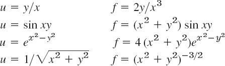
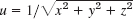
In general, the totality of solutions of a PDE is very large. For example, the functions
![]()
which are entirely different from each other, are solutions of (3), as you may verify. We shall see later that the unique solution of a PDE corresponding to a given physical problem will be obtained by the use of additional conditions arising from the problem. For instance, this may be the condition that the solution u assume given values on the boundary of the region R (“boundary conditions”). Or, when time t is one of the variables, u (ut = ∂u/∂t or both) may be prescribed at t = 0 (“initial conditions”).
We know that if an ODE is linear and homogeneous, then from known solutions we can obtain further solutions by superposition. For PDEs the situation is quite similar:
THEOREM 1 Fundamental Theorem on Superposition
If u1 and u2 are solutions of a homogeneous linear PDE in some region R, then
![]()
with any constants c1 and c2 is also a solution of that PDE in the region R.
The simple proof of this important theorem is quite similar to that of Theorem 1 in Sec. 2.1 and is left to the student.
Verification of solutions in Probs. 2–13 proceeds as for ODEs. Problems 16–23 concern PDEs solvable like ODEs. To help the student with them, we consider two typical examples.
EXAMPLE 2 Solving uxx − u = 0 Like an ODE
Find solutions u of the PDE uxx − u = 0 depending on x and y.
Solution. Since no y-derivatives occur, we can solve this PDE like un − u = 0. In Sec. 2.2 we would have obtained u = Aex + Be−x with constant A and B. Here A and B may be functions of y, so that the answer is
![]()
with arbitrary functions A and B. We thus have a great variety of solutions. Check the result by differentiation.
EXAMPLE 3 Solving uxy = −ux Like an ODE
Find solutions u = u(x, y) of this PDE.
Solution. Setting ux = p, we have py = −p, py/p = −1, ln |p| = −y + c~(x), p = c(x)e−y and by integration with respect to x,
here, f(x) and g(y) are arbitrary.
- Fundamental theorem. Prove it for second-order PDEs in two and three independent variables. Hint. Prove it by substitution.
2.13 VERIFICATION OF SOLUTIONS
Verifiy (by substitution) that the given function is a solution of the PDE. Sketch or graph the solution as a surface in space.
2.5 Wave Equation (1) with suitable c
- 2. u = x2 + t2
- 3. u = cos 4t sin 2x
- 4. u = sin kct cos x
- 5. u = sin at sin bx
6.9 Heat Equation (2) with suitable c
- 6. u = e−t sin x
- 7.

- 8.

- 9.
10.13 Laplace Equation (3)
- 10. u = ex cos y, ex sin y
- 11. u = arctan (y/x)
- 12. u = cos y sinh x, sin y cosh x
- 13. u = x/(x2 + y2),y/(y2 + y2)
- 14. TEAM PROJECT. Verification of Solutions
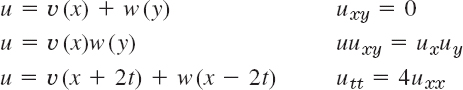
- Wave equation. Verify that u(x, t) = ν(x + ct) + w(x − ct) with any twice differentiable functions v and w satisfies (1).
- Poisson equation. Verify that each u satisfies (4) with as indicated.
- Laplace equation. Verify that
 satisfies (6) and u = ln (x2 + y2) satisfies (3). Is
 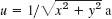 a solution of (3)? Of what Poisson equation?
 - Verify that u with any (sufficiently often differentiable) v and w satisfies the given PDE.
- 15. Boundary value problem. Verify that the function satisfies Laplace's equation u(x, y) = a ln (x2 + y2) + b statisfies Laplace's equation (3) and determine a and b so that u satisfies the boundary conditions u = 110 on the circle x2 + y2 and u = 0 on the circle x2 + y2 = 100.
16.23 PDEs SOLVABLE AS ODEs
This happens if a PDE involves derivatives with respect to one variable only (or can be transformed to such a form), so that the other variable(s) can be treated as parameter(s). Solve for u = u(x, y):
- 16. uyy = 0
- 17. uxx + 16π2u = 0
- 18. 25uyy − 4u = 0
- 19. uy + y2u = 0
- 20. 2uxx + 9ux + 4u = −3 cos x − 29 sin x
- 21. uxy + 6uy + 13u = 4e3y
- 22. uxy = ux
- 23. x2uxx + 2xux − 2u = 0
- 24. Surface of revolution. Show that the solutions z = z(x, y) of yzx = xzy represent surfaces of revolution. Give examples. Hint. Use polar coordinates r, θ and show that the equation becomes zθ = 0.
- 25. System of PDEs. Solve uxx = 0, uyy = 0
12.2 Modeling: Vibrating String, Wave Equation
In this section we model a vibrating string, which will lead to our first important PDE, that is, equation (3) which will then be solved in Sec. 12.3. The student should pay very close attention to this delicate modeling process and detailed derivation starting from scratch, as the skills learned can be applied to modeling other phenomena in general and in particular to modeling a vibrating membrane (Sec. 12.7).
We want to derive the PDE modeling small transverse vibrations of an elastic string, such as a violin string. We place the string along the x-axis, stretch it to length L, and fasten it at the ends x = 0 and x = L. We then distort the string, and at some instant, call it t = 0, we release it and allow it to vibrate. The problem is to determine the vibrations of the string, that is, to find its deflection u(x, t) at any point x and at any time t > 0; see Fig. 286.
u(x, t) will be the solution of a PDE that is the model of our physical system to be derived. This PDE should not be too complicated, so that we can solve it. Reasonable simplifying assumptions (just as for ODEs modeling vibrations in Chap. 2) are as follows.
Physical Assumptions
- The mass of the string per unit length is constant (“homogeneous string”). The string is perfectly elastic and does not offer any resistance to bending.
- The tension caused by stretching the string before fastening it at the ends is so large that the action of the gravitational force on the string (trying to pull the string down a little) can be neglected.
- The string performs small transverse motions in a vertical plane; that is, every particle of the string moves strictly vertically and so that the deflection and the slope at every point of the string always remain small in absolute value.
Under these assumptions we may expect solutions that describe the physical reality sufficiently well.

Fig. 286. Deflected string at fixed time t. Explanation on p. 544
Derivation of the PDE of the Model (“Wave Equation”) from Forces
The model of the vibrating string will consist of a PDE (“wave equation”) and additional conditions. To obtain the PDE, we consider the forces acting on a small portion of the string (Fig. 286). This method is typical of modeling in mechanics and elsewhere.
Since the string offers no resistance to bending, the tension is tangential to the curve of the string at each point. Let T1 and T2 be the tension at the endpoints P and Q of that portion. Since the points of the string move vertically, there is no motion in the horizontal direction. Hence the horizontal components of the tension must be constant. Using the notation shown in Fig. 286, we thus obtain
![]()
In the vertical direction we have two forces, namely, the vertical components −T1 sin α and T2 sin β of T1 and T2; here the minus sign appears because the component at P is directed downward. By Newton's second law (Sec. 2.4) the resultant of these two forces is equal to the mass ρΔx of the portion times the acceleration ∂2u/∂t2, evaluated at some point between x and x + Δx; here ρ is the mass of the undeflected string per unit length, and Δx is the length of the portion of the undeflected string. (Δ is generally used to denote small quantities; this has nothing to do with the Laplacian ![]() , which is sometimes also denoted by Δ) Hence
, which is sometimes also denoted by Δ) Hence
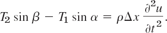
Using (1), we can divide this by T2 cos β = T1 cos α = T, obtaining

Now tan α and tan β are the slopes of the string at x and x + Δx:

Here we have to write partial derivatives because u also depends on time t. Dividing (2) by Δx, we thus have
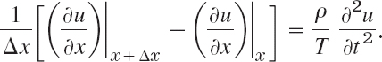
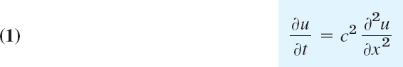
If we let Δx approach zero, we obtain the linear PDE

This is called the one-dimensional wave equation. We see that it is homogeneous and of the second order. The physical constant T/ρ is denoted by c2 (instead of c) to indicate that this constant is positive, a fact that will be essential to the form of the solutions. “One-dimensional” means that the equation involves only one space variable, x. In the next section we shall complete setting up the model and then show how to solve it by a general method that is probably the most important one for PDEs in engineering mathematics.
12.3 Solution by Separating Variables. Use of Fourier Series
We continue our work from Sec. 12.2, where we modeled a vibrating string and obtained the one-dimensional wave equation. We now have to complete the model by adding additional conditions and then solving the resulting model.
The model of a vibrating elastic string (a violin string, for instance) consists of the one-dimensional wave equation
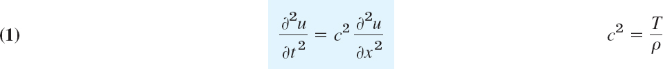
for the unknown deflection u(x, t) of the string, a PDE that we have just obtained, and some additional conditions, which we shall now derive.
Since the string is fastened at the ends x = 0 and x = L (see Sec. 12.2), we have the two boundary conditions

Furthermore, the form of the motion of the string will depend on its initial deflection (deflection at time t = 0), call it f(x), and on its initial velocity (velocity at t = 0), call it g(x). We thus have the two initial conditions

where ut = ∂u/∂t. We now have to find a solution of the PDE (1) satisfying the conditions (2) and (3). This will be the solution of our problem. We shall do this in three steps, as follows.
Step 1. By the “method of separating variables” or product method, setting u(x, t) = F(x)G(t), we obtain from (1) two ODEs, one for F(x) and the other one for G(t).
Step 2. We determine solutions of these ODEs that satisfy the boundary conditions (2).
Step 3. Finally, using Fourier series, we compose the solutions found in Step 2 to obtain a solution of (1) satisfying both (2) and (3), that is, the solution of our model of the vibrating string.
Step 1. Two ODEs from the Wave Equation (1)
In the method of separating variables, or product method, we determine solutions of the wave equation (1) of the form

which are a product of two functions, each depending on only one of the variables x and t. This is a powerful general method that has various applications in engineering mathematics, as we shall see in this chapter. Differentiating (4), we obtain
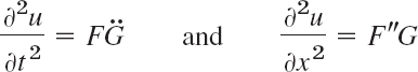
where dots denote derivatives with respect to t and primes derivatives with respect to x. By inserting this into the wave equation (1) we have
![]()
Dividing by c2FG and simplifying gives
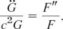
The variables are now separated, the left side depending only on t and the right side only on x. Hence both sides must be constant because, if they were variable, then changing t or x would affect only one side, leaving the other unaltered. Thus, say,
Multiplying by the denominators gives immediately two ordinary DEs

and
Here, the separation constant k is still arbitrary.
Step 2. Satisfying the Boundary Conditions (2)
We now determine solutions F and G of (5) and (6) so that u = FG satisfies the boundary conditions (2), that is,
![]()
We first solve (5). If G ≡, then u = FG ≡ 0, which is of no interest. Hence G ≡ 0 and then by (7),
![]()
We show that k must be negative. For k = 0 the general solution of (5) is F = ax + b, and from (8) we obtain a = b = 0, so that F ≡ 0 and u = FG ≡ 0, which is of no interest. For positive k = μ2 a general solution of (5) is
![]()
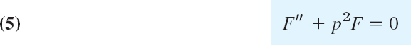
and from (8) we obtain F ≡ 0 as before (verify!). Hence we are left with the possibility of choosing k negative, say, k = −p2. Then (5) becomes F″ + p2F = 0 and has as a general solution
![]()
From this and (8) we have
![]()
We must take B ≠ 0 since otherwise F ≡ 0. Hence sin pL = 0. Thus
![]()
Setting B = 1 we thus obtain infinitely many solutions F(x) = Fn(x) where
![]()
These solutions satisfy (8). [For negative integer n we obtain essentially the same solutions, except for a minus sign, because sin (−α) = −sin α.]
We now solve (6) with k = −p2 = −(nπ/L2) resulting from (9), that is,
![]()
A general solution is
![]()
Hence solutions of (1) satisfying (2) are un(x, t) = Fn(x)Gn(t) = Gn(t)Fn(x), written out

These functions are called the eigenfunctions, or characteristic functions, and the values λn = cnπ/L are called the eigenvalues, or characteristic values, of the vibrating string. The set {λ1, λ2, …} is called the spectrum.
Discussion of Eigenfunctions. We see that each un represents a harmonic motion having the frequency λn/2π = cn/2L cycles per unit time. This motion is called the nth normal mode of the string. The first normal mode is known as the fundamental mode and the others are known as overtones; musically they give the octave, octave plus fifth, etc. Since in (11)
![]()
the nth normal mode has n − 1 nodes, that is, points of the string that do not move (in addition to the fixed endpoints); see Fig. 287.

Fig. 287. Normal modes of the vibrating string
Figure 288 shows the second normal mode for various values of t. At any instant the string has the form of a sine wave. When the left part of the string is moving down, the other half is moving up, and conversely. For the other modes the situation is similar.
Tuning is done by changing the tension T. Our formula for the frequency λn/2π = cn/2L of un with ![]() [see (3), Sec. 12.2] confirms that effect because it shows that the frequency is proportional to the tension. T cannot be increased indefinitely, but can you see what to do to get a string with a high fundamental mode? (Think of both L and ρ.) Why is a violin smaller than a double-bass?
[see (3), Sec. 12.2] confirms that effect because it shows that the frequency is proportional to the tension. T cannot be increased indefinitely, but can you see what to do to get a string with a high fundamental mode? (Think of both L and ρ.) Why is a violin smaller than a double-bass?
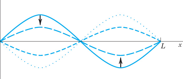
Fig. 288. Second normal mode for various values of t
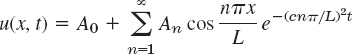
Step 3. Solution of the Entire Problem. Fourier Series
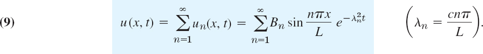
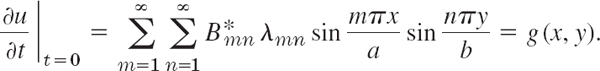
The eigenfunctions (11) satisfy the wave equation (1) and the boundary conditions (2) (string fixed at the ends). A single un will generally not satisfy the initial conditions (3). But since the wave equation (1) is linear and homogeneous, it follows from Fundamental Theorem 1 in Sec. 12.1 that the sum of finitely many solutions un is a solution of (1). To obtain a solution that also satisfies the initial conditions (3), we consider the infinite series (with λn = cnπ/L as before)

Satisfying Initial Condition (3a) (Given Initial Displacement). From (12) and (3a) we obtain

Hence we must choose the Bn*'s so that u(x, 0) becomes the Fourier sine series of f(x). Thus, by (4) in Sec. 11.3,

Satisfying Initial Condition (3b) (Given Initial Velocity). Similarly, by differentiating (12) with respect to t and using (3b), we obtain

Hence we must choose the ![]() so that for t = 0 the derivative ∂u/∂t becomes the Fourier sine series of g(x). Thus, again by (4) in Sec. 11.3,
so that for t = 0 the derivative ∂u/∂t becomes the Fourier sine series of g(x). Thus, again by (4) in Sec. 11.3,
Since λn = cnπ/L, we obtain by division

Result. Our discussion shows that u(x, t) given by (12) with coefficients (14) and (15) is a solution of (1) that satisfies all the conditions in (2) and (3), provided the series (12) converges and so do the series obtained by differentiating (12) twice termwise with respect to x and t and have the sums ∂2u/∂x2 and ∂2u/∂t2, respectively, which are continuous.
Solution (12) Established. According to our derivation, the solution (12) is at first a purely formal expression, but we shall now establish it. For the sake of simplicity we consider only the case when the initial velocity g(x) is identically zero. Then the Bn* are zero, and (12) reduces to

It is possible to sum this series, that is, to write the result in a closed or finite form. For this purpose we use the formula [see (11), App. A3.1]

Consequently, we may write (16) in the form

These two series are those obtained by substituting x − ct and x + ct, respectively, for the variable x in the Fourier sine series (13) for f(x). Thus

where f* is the odd periodic extension of f with the period 2L (Fig. 289). Since the initial deflection f(x) is continuous on the interval 0 ![]() x
x ![]() L and zero at the endpoints, it follows from (17) that u(x, t) is a continuous function of both variables x and t for all values of the variables. By differentiating (17) we see that u(x, t) is a solution of (1), provided f(x) is twice differentiable on the interval 0 < x < L, and has one-sided second derivatives at x = 0 and x = L, which are zero. Under these conditions u(x, t) is established as a solution of (1), satisfying (2) and (3) with g(x) ≡ 0.
L and zero at the endpoints, it follows from (17) that u(x, t) is a continuous function of both variables x and t for all values of the variables. By differentiating (17) we see that u(x, t) is a solution of (1), provided f(x) is twice differentiable on the interval 0 < x < L, and has one-sided second derivatives at x = 0 and x = L, which are zero. Under these conditions u(x, t) is established as a solution of (1), satisfying (2) and (3) with g(x) ≡ 0.
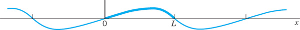
Fig. 289. Odd periodic extension of f(x)
Generalized Solution. If f′(x) and f″(x) are merely piecewise continuous (see Sec. 6.1), or if those one-sided derivatives are not zero, then for each t there will be finitely many values of x at which the second derivatives of u appearing in (1) do not exist. Except at these points the wave equation will still be satisfied. We may then regard u(x, t) as a “generalized solution,” as it is called, that is, as a solution in a broader sense. For instance, a triangular initial deflection as in Example 1 (below) leads to a generalized solution.
Physical Interpretation of the Solution (17). The graph of f* (x − ct) is obtained from the graph of f*(x) by shifting the latter ct units to the right (Fig. 290). This means that f*(x − ct)(c > 0) represents a wave that is traveling to the right as t increases. Similarly, f*(x + ct) represents a wave that is traveling to the left, and u(x, t) is the superposition of these two waves.

Fig. 290. Interpretation of (17)
EXAMPLE 1 Vibrating String if the Initial Deflection Is Triangular
Find the solution of the wave equation (1) satisfying (2) and corresponding to the triangular initial deflection
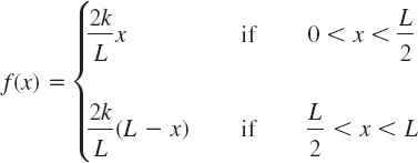
and initial velocity zero. (Figure 291 shows f(x) = u(x, 0) at the top.)
Solution. Since g(x) ≡ we have ![]() in (12), and from Example 4 in Sec. 11.3 we see that the Bn are given by (5), Sec. 11.3. Thus (12) takes the form
in (12), and from Example 4 in Sec. 11.3 we see that the Bn are given by (5), Sec. 11.3. Thus (12) takes the form

For graphing the solution we may use u(x, 0) = f(x) and the above interpretation of the two functions in the representation (17). This leads to the graph shown in Fig. 291.

Fig. 291. Solution u(x, t) in Example 1 for various values of t (right part of the figure) obtained as the superposition of a wave traveling to the right (dashed) and a wave traveling to the left (left part of the figure)
- Frequency. How does the frequency of the fundamental mode of the vibrating string depend on the length of the string? On the mass per unit length? What happens if we double the tension? Why is a contrabass larger than a violin?
- Physical Assumptions. How would the motion of the string change if Assumption 3 were violated? Assumption 2? The second part of Assumption 1? The first part? Do we really need all these assumptions?
- String of length π. Write down the derivation in this section for length L = π, to see the very substantial simplification of formulas in this case that may show ideas more clearly.
- CAS PROJECT. Graphing Normal Modes. Write a program for graphing un with L = π and c2 of your choice similarly as in Fig. 287. Apply the program to u2, u3, u4. Also graph these solutions as surfaces over the xt-plane. Explain the connection between these two kinds of graphs.
5.13 DEFLECTION OF THE STRING
Find u(x, t) for the string of length L = 1 and c2 when the initial velocity is zero and the initial deflection with small k (say, 0.01) is as follows. Sketch or graph u(x, t) as in Fig. 291 in the text.
- 5. k sin 3πx
- 6.
- 7. kx(1 − x)
- 8. kx2(1 − x)
- 9.

- 10.
- 11.

- 12.

- 13. 2x − 4x2 if
- 14. Nonzero initial velocity. Find the deflection of u(x, t) of the string of length L = π and c2 = 1 for for zero initial displacement and “triangular” initial velocity ut(x, 0) = 0.01x if
 , ut(x, 0) = 0.01(π − x) if
 x π. (Initial conditions with ut(x, 0) ≠ 0 are hard to realize experimentally.)

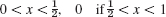
15.20 SEPARATION OF A FOURTH-ORDER PDE. VIBRATING BEAM
By the principles used in modeling the string it can be shown that small free vertical vibrations of a uniform elastic beam (Fig. 292) are modeled by the fourth-order PDE

where c2 = EI/ρA (E = Young's modulus of elasticity, I = movement of intertia of the cross section with respect to the y-axis in the figure, ρ = density, A = cross-sectional area.) (Bending of a beam under a load is discussed in Sec. 3.3.)
- 15. Subtituting u = F(x)G(t) into (21), show that

- 16. Simply supported beam in Fig. 293A. Find solutions un = Fn(x)Gn(t) of (21) corresponding to zero initial velocity and satisfying the boundary conditions (see Fig. 293A)
- 17. Find the solution of (21) that satisfies the conditions in Prob. 16 as well as the initial condition

- 18. Compare the results of Probs. 17 and 7. What is the basic difference between the frequencies of the normal modes of the vibrating string and the vibrating beam?
- 19. Clamped beam in Fig. 293B. What are the boundary conditions for the clamped beam in Fig. 293B? Show that F in Prob. 15 satisfies these conditions if βL is a solution of the equation

Determine approximate solutions of (22), for instance, graphically from the intersections of the curves of cos βL and 1/cosh βL.
- 20. Clamped-free beam in Fig. 293C. If the beam is clamped at the left and free at the right (Fig. 293C), the boundary conditions are

Show that F in Prob. 15 satisfies these conditions if βL is a solution of the equation

Find approximate solutions of (23).
12.4 D'Alembert's Solution of the Wave Equation. Characteristics
It is interesting that the solution (17), Sec. 12.3, of the wave equation

can be immediately obtained by transforming (1) in a suitable way, namely, by introducing the new independent variables
![]()
Then u becomes a function of v and w. The derivatives in (1) can now be expressed in terms of derivatives with respect to v and w by the use of the chain rule in Sec. 9.6. Denoting partial derivatives by subscripts, we see from (2) that vx = 1 and wx = 1. For simplicity let us denote u(x, t) as a function of v and w, by the same letter u. Then
![]()
We now apply the chain rule to the right side of this equation. We assume that all the partial derivatives involved are continuous, so that uwv = uvw. Since vx = 1 and wx = 1 we obtain
![]()
Transforming the other derivative in (1) by the same procedure, we find
![]()
By inserting these two results in (1) we get (see footnote 2 in App. A3.2)

The point of the present method is that (3) can be readily solved by two successive integrations, first with respect to w and then with respect to v. This gives

Here h(v) and ψ(w) are arbitrary functions of v and w, respectively. Since the integral is a function of v, say, φ(v), the solution is of the form u = φ(v) + ψ(w). In terms of x and t, by (2), we thus have

This is known as d'Alembert's solution1 of the wave equation (1).
Its derivation was much more elegant than the method in Sec. 12.3, but d'Alembert's method is special, whereas the use of Fourier series applies to various equations, as we shall see.
D'Alembert's Solution Satisfying the Initial Conditions
![]()
These are the same as (3) in Sec. 12.3. By differentiating (4) we have
![]()
where primes denote derivatives with respect to the entire arguments x + ct and x − ct, respectively, and the minus sign comes from the chain rule. From (4)–(6) we have
![]()
![]()
Dividing (8) by c and integrating with respect to x, we obtain

If we add this to (7), then ψ drops out and division by 2 gives

Similarly, subtraction of (9) from (7) and division by 2 gives

In (10) we replace x by x + ct; we then get an integral from to x0 to x + ct. In (11) we replace x by x − ct and get minus an integral from x0 to x − ct or plus an integral from x − ct to x0. Hence addition of φ(x + ct) and ψ(x − ct) gives u(x, t) [see (4)] in the form

If the initial velocity is zero, we see that this reduces to
![]()
in agreement with (17) in Sec. 12.3. You may show that because of the boundary conditions (2) in that section the function f must be odd and must have the period 2L.
Our result shows that the two initial conditions [the functions f(x) and g(x) in (5)] determine the solution uniquely.
The solution of the wave equation by the Laplace transform method will be shown in Sec. 12.11.
Characteristics. Types and Normal Forms of PDEs
The idea of d'Alembert's solution is just a special instance of the method of characteristics. This concerns PDEs of the form

(as well as PDEs in more than two variables). Equation (14) is called quasilinear because it is linear in the highest derivatives (but may be arbitrary otherwise). There are three types of PDEs (14), depending on the discriminant AC − B2, as follows.
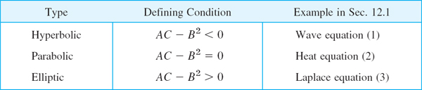
Note that (1) and (2) in Sec. 12.1 involve t, but to have y as in (14), we set y = ct in (1), obtaining utt − c2uxx = c2(uyy − uxx) = 0. And in (2) we set y = c2t, so that ut − c2uxx = c2(uy − uxx).
A, B, C may be functions of x, y, so that a PDE may be of mixed type, that is, of different type in different regions of the xy-plane. An important mixed-type PDE is the Tricomi equation (see Prob. 10).
Transformation of (14) to Normal Form. The normal forms of (14) and the corresponding transformations depend on the type of the PDE. They are obtained by solving the characteristic equation of (14), which is the ODE
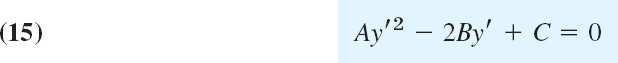
where y′ = dy/dx (note −2B, not + 2B). The solutions of (15) are called the characteristics of (14), and we write them in the form Φ(x, y) = const and Ψ(x, y) = const. Then the transformations giving new variables v, w instead of x, y and the normal forms of (14) are as follows.

Here, Φ = Φ(x, y), Ψ = Ψ(x, y), F1 = F1(u, w, u, uv, uw), etc., and we denote u as function of v, w again by u, for simplicity. We see that the normal form of a hyperbolic PDE is as in d'Alembert's solution. In the parabolic case we get just one family of solutions Φ = Ψ. In the elliptic case, ![]() , and the characteristics are complex and are of minor interest. For derivation, see Ref. [GenRef3] in App. 1.
, and the characteristics are complex and are of minor interest. For derivation, see Ref. [GenRef3] in App. 1.
EXAMPLE 1 D'Alembert's Solution Obtained Systematically
The theory of characteristics gives d'Alembert's solution in a systematic fashion. To see this, we write the wave equation utt − c2uxx = 0 in the form (14) by setting y = ct. By the chain rule, ut = uyyt = cuy and utt = c2uyy. Division by c2 gives uxx − uyy = 0, as stated before. Hence the characteristic equation is y′2 − 1 = (y′ + 1)(y′ − 1) = 0. The two families of solutions (characteristics) are Φ(x, y) = y + x = const and Ψ(x, y) = y − x = const. This gives the new variables v = Φ = y + x = ct + x and w = Ψ = y − x = ct − x and d'Alembert's solution u = f1(x + ct) + f2(x − ct).
- Show that c is the speed of each of the two waves given by (4).
- Show that, because of the boundary conditions (2), Sec. 12.3, the function f in (13) of this section must be odd and of period 2L.
- If a steel wire 2 m in length weighs 0.9 nt (about 0.20 lb) and is stretched by a tensile force of 300 nt (about 67.4 lb), what is the corresponding speed of transverse waves?
- What are the frequencies of the eigenfunctions in Prob. 3?
5.8 GRAPHING SOLUTIONS
Using (13) sketch or graph a figure (similar to Fig. 291 in Sec. 12.3) of the deflection u(x, t) of a vibrating string (length L = 1, ends fixed, c = 1) starting with initial velocity 0 and initial deflection (k small, say, k = 0.01).
- 5. f(x) = k sin πx
- 6. f(x) = k sin 2πx
- 7. f(x) = k(1 − cos πx)
- 8. f(x) = kx(1 − x)
9.18 NORMAL FORMS
Find the type, transform to normal form, and solve. Show your work in detail.
- 9. uxx + 4uyy = 0
- 10. uxx − 16uyy = 0
- 11. uxx + 2uxy + uyy = 0
- 12. uxx − 2uxy + uyy = 0
- 13. uxx + 5uxy + 4uyy = 0
- 14. xuxy − yuyy = 0
- 15. xuxx − yuxy = 0
- 16. uxx + 2uxy + 10uyy = 0
- 17. uxx − 4uxy + 5uyy = 0
- 18. uxx − 6uxy + 9uyy = 0
- 19. Longitudinal Vibrations of an Elastic Bar or Rod. These vibrations in the direction of the x-axis are modeled by the wave equation utt = c2uxx, c2 = E/ρ (see Tolstov [C9], p. 275). If the rod is fastened at one end, x = 0, and free at the other, x = L, we have u(0, t) = 0 and ux(L, t) = 0. Show that the motion corresponding to initial displacement u(x, 0) = f(x) and initial velocity zero is

- 20. Tricomi and Airy equations.2 Show that the Tricomi equation yuxx + uyy = 0 is of mixed type. Obtain the Airy equation G″ − yG = 0 from the Tricomi equation by separation. (For solutions, see p. 446 of Ref. [GenRef1] listed in App. 1.)
12.5 Modeling: Heat Flow from a Body in Space. Heat Equation
After the wave equation (Sec. 12.2) we now derive and discuss the next “big” PDE, the heat equation, which governs the temperature u in a body in space. We obtain this model of temperature distribution under the following.
Physical Assumptions
- The specific heat σ and the density ρ of the material of the body are constant. No heat is produced or disappears in the body.
- Experiments show that, in a body, heat flows in the direction of decreasing temperature, and the rate of flow is proportional to the gradient (cf. Sec. 9.7) of the temperature; that is, the velocity v of the heat flow in the body is of the form

where u(x, y, z, t) is the temperature at a point (x, y, z) and time t.
- The thermal conductivity K is constant, as is the case for homogeneous material and nonextreme temperatures.
Under these assumptions we can model heat flow as follows.
Let T be a region in the body bounded by a surface S with outer unit normal vector n such that the divergence theorem (Sec. 10.7) applies. Then
![]()
is the component of v in the direction of n. Hence |v • n ΔA| is the amount of heat leaving T (if v • n > 0 at some point P) or entering T (if v • n < 0 at P) per unit time at some point P of S through a small portion ΔS of s of area ΔA. Hence the total amount of heat that flows across S from T is given by the surface integral

Note that, so far, this parallels the derivation on fluid flow in Example 1 of Sec. 10.8.
Using Gauss's theorem (Sec. 10.7), we now convert our surface integral into a volume integral over the region T. Because of (1) this gives [use (3) in Sec. 9.8]
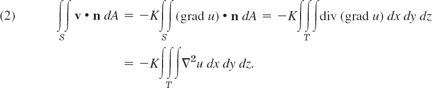
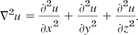
Here,
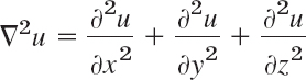
is the Laplacian of u.
On the other hand, the total amount of heat in T is

with σ and ρ as before. Hence the time rate of decrease of H is
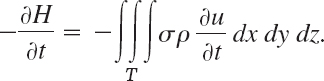
This must be equal to the amount of heat leaving T because no heat is produced or disappears in the body. From (2) we thus obtain
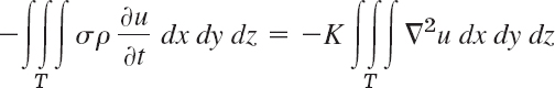
or (divide by −σρ)

Since this holds for any region T in the body, the integrand (if continuous) must be zero everywhere. That is,

This is the heat equation, the fundamental PDE modeling heat flow. It gives the temperature u(x, y, z, t) in a body of homogeneous material in space. The constant c2 is the thermal diffusivity. K is the thermal conductivity, σ the specific heat, and ρ the density of the material of the body. ![]() is the Laplacian of u and, with respect to the Cartesian coordinates x, y, z, is
is the Laplacian of u and, with respect to the Cartesian coordinates x, y, z, is
The heat equation is also called the diffusion equation because it also models chemical diffusion processes of one substance or gas into another.
12.6 Heat Equation: Solution by Fourier Series. Steady Two-Dimensional Heat Problems. Dirichlet Problem
We want to solve the (one-dimensional) heat equation just developed in Sec. 12.5 and give several applications. This is followed much later in this section by an extension of the heat equation to two dimensions.

Fig. 294. Bar under consideration
As an important application of the heat equation, let us first consider the temperature in a long thin metal bar or wire of constant cross section and homogeneous material, which is oriented along the x-axis (Fig. 294) and is perfectly insulated laterally, so that heat flows in the x-direction only. Then besides time, u depends only on x, so that the Laplacian reduces to uxx = ∂2u = ∂2u/∂x2, and the heat equation becomes the one-dimensional heat equation
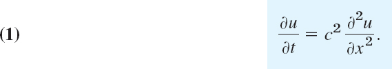
This PDE seems to differ only very little from the wave equation, which has a term utt instead of ut, but we shall see that this will make the solutions of (1) behave quite differently from those of the wave equation.
We shall solve (1) for some important types of boundary and initial conditions. We begin with the case in which the ends x = 0 and x = L of the bar are kept at temperature zero, so that we have the boundary conditions

Furthermore, the initial temperature in the bar at time t = 0 is given, say, f(x), so that we have the initial condition

Here we must have f(0) = 0 and f(L) = 0 because of (2).
We shall determine a solution u(x, t) of (1) satisfying (2) and (3)—one initial condition will be enough, as opposed to two initial conditions for the wave equation. Technically, our method will parallel that for the wave equation in Sec. 12.3: a separation of variables, followed by the use of Fourier series. You may find a step-by-step comparison worthwhile.
Step 1. Two ODEs from the heat equation (1). Substitution of a product u(x, t) = F(x)G(t) into (1) gives ![]() with
with ![]() and F″ = d2F/dx2. To separate the variables, we divide c2FG by obtaining
and F″ = d2F/dx2. To separate the variables, we divide c2FG by obtaining

The left side depends only on t and the right side only on x, so that both sides must equal a constant k (as in Sec. 12.3). You may show that for k = 0 or k > 0 the only solution u = FG satisfying (2) is u ≡ 0. For negative k = −p2 we have from (4)
Multiplication by the denominators immediately gives the two ODEs
and

Step 2. Satisfying the boundary conditions (2). We first solve (5). A general solution is
![]()
From the boundary conditions (2) it follows that
![]()
Since G ≡ 0 would give u ≡ 0, we require F(0) = 0, F(L) = 0 and get F(0) = A = 0 by (7) and then F(L) = B sin pL = 0, with B ≠ 0 (to avoid F ≡ 0); thus,
![]()
Setting B = 1, we thus obtain the following solutions of (5) satisfying (2):
![]()
(As in Sec. 12.3, we need not consider negative integer values of n.)
All this was literally the same as in Sec. 12.3. From now on it differs since (6) differs from (6) in Sec. 12.3. We now solve (6). For p = nπ/L, as just obtained, (6) becomes
![]()
It has the general solution
![]()
where Bn is a constant. Hence the functions

are solutions of the heat equation (1), satisfying (2). These are the eigenfunctions of the problem, corresponding to the eigenvalues λn = cnπ/L.
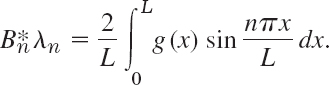
Step 3. Solution of the entire problem. Fourier series. So far we have solutions (8) satisfying the boundary conditions (2). To obtain a solution that also satisfies the initial condition (3), we consider a series of these eigenfunctions,

Hence for (9) to satisfy (3), the Bn's must be the coefficients of the Fourier sine series, as given by (4) in Sec. 11.3; thus
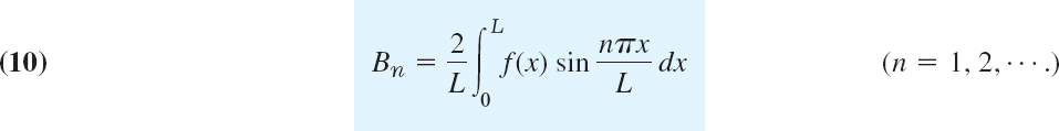
The solution of our problem can be established, assuming that f(x) is piecewise continuous (see Sec. 6.1) on the interval 0 ![]() x
x ![]() L and has one-sided derivatives (see Sec. 11.1) at all interior points of that interval; that is, under these assumptions the series (9) with coefficients (10) is the solution of our physical problem. A proof requires knowledge of uniform convergence and will be given at a later occasion (Probs. 19, 20 in Problem Set 15.5).
L and has one-sided derivatives (see Sec. 11.1) at all interior points of that interval; that is, under these assumptions the series (9) with coefficients (10) is the solution of our physical problem. A proof requires knowledge of uniform convergence and will be given at a later occasion (Probs. 19, 20 in Problem Set 15.5).
Because of the exponential factor, all the terms in (9) approach zero as t approaches infinity. The rate of decay increases with n.
EXAMPLE 1 Sinusoidal Initial Temperature
Find the temperature u(x, t) in a laterally insulated copper bar 80 cm long if the initial temperature is 100 sin(πx/80) °C and the ends are kept at 0°C. How long will it take for the maximum temperature in the bar to drop to 50°C? First guess, then calculate. Physical data for copper: density 8.92 g/cm3, specific heat 0.092 cal/(g °C) thermal conductivity 0.95 cal/(cm sec °C).
Solution. The initial condition gives

Hence, by inspection or from (9), we get B1 = 100, B2 = B3 = … = 0. In (9) we need ![]() , where c2 = K/(σρ) = 0.95/(0.092 · 8.92) = 1.158 [cm2/sec]. Hence we obtain
, where c2 = K/(σρ) = 0.95/(0.092 · 8.92) = 1.158 [cm2/sec]. Hence we obtain
![]()
The solution (9) is
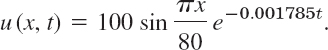
Also, 100e−0.001785t = 50 when t = (ln 0.5)/(−0.001785) = 388[sec] ≈ 6.5 [min]. Does your guess, or at least its order of magnitude, agree with this result?
Solve the problem in Example 1 when the initial temperature is 100 sin(3πx/80) °C and the other data are as before.
Solution. In (9), instead of n = 1 we now have n = 3, and ![]() , so that the solution now is
, so that the solution now is

Hence the maximum temperature drops to 50°C in t = (ln 0.5)/(−0.01607) ≈ 43 [sec], which is much faster (9 times as fast as in Example 1; why?).
Had we chosen a bigger n, the decay would have been still faster, and in a sum or series of such terms, each term has its own rate of decay, and terms with large n are practically 0 after a very short time. Our next example is of this type, and the curve in Fig. 295 corresponding to t = 0.5 looks almost like a sine curve; that is, it is practically the graph of the first term of the solution.
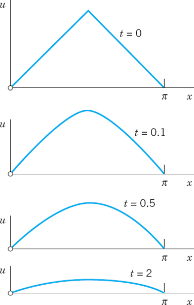
Fig. 295. Example 3. Decrease of temperature with time t for and L = π and c = 1
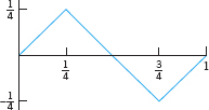
EXAMPLE 3 “Triangular” Initial Temperature in a Bar
Find the temperature in a laterally insulated bar of length L whose ends are kept at temperature 0, assuming that the initial temperature is
(The uppermost part of Fig. 295 shows this function for the special L = π.)
Solution. From (10) we get

Integration gives if Bn = 0 if n is even,
![]()
(see also Example 4 in Sec. 11.3 with k = L/2). Hence the solution is
![]()
Figure 295 shows that the temperature decreases with increasing t, because of the heat loss due to the cooling of the ends.
EXAMPLE 4 Bar with Insulated Ends. Eigenvalue 0
Find a solution formula of (1), (3) with (2) replaced by the condition that both ends of the bar are insulated.
Solution. Physical experiments show that the rate of heat flow is proportional to the gradient of the temperature. Hence if the ends x = 0 and x = L of the bar are insulated, so that no heat can flow through the ends, we have grad u = ux = ∂u/∂x and the boundary conditions
![]()
Since u(x, t) = F(x)G(t), this gives ux(0, t) = F′(0)G(t) = 0 and ux(L, t) = F′(L)G(t) = 0. Differentiating (7), we have F′(x) = −Ap sin px + Bp cos px, so that
![]()
The second of these conditions gives p = pn = nπ/L, (n = 0, 1, 2, …) From this and (7) with A = 1 and B = 0 we get Fn(x) = cos(nπx/L), (n = 0, 1, 2, …). With Gn as before, this yields the eigenfunctions
![]()
corresponding to the eigenvalues λn = cnπ/L. The latter are as before, but we now have the additional eigenvalue λ0 = 0 and eigenfunction u0 = const, which is the solution of the problem if the initial temperature f(x) is constant. This shows the remarkable fact that a separation constant can very well be zero, and zero can be an eigenvalue.
Furthermore, whereas (8) gave a Fourier sine series, we now get from (11) a Fourier cosine series

Its coefficients result from the initial condition (3),
in the form (2), Sec. 11.3, that is,

EXAMPLE 5 “Triangular” Initial Temperature in a Bar with Insulated Ends
Find the temperature in the bar in Example 3, assuming that the ends are insulated (instead of being kept at temperature 0).
Solution. For the triangular initial temperature, (13) gives A0 = L/4 and (see also Example 4 in Sec. 11.3 with k = L/2)

Hence the solution (12) is

We see that the terms decrease with increasing t, and u → L/4 as t → ∞; this is the mean value of the initial temperature. This is plausible because no heat can escape from this totally insulated bar. In contrast, the cooling of the ends in Example 3 led to heat loss and, the temperature at which the ends were kept.
Steady Two-Dimensional Heat Problems. Laplace's Equation
We shall now extend our discussion from one to two space dimensions and consider the two-dimensional heat equation

for steady (that is, time-independent) problems. Then ∂u/∂t = 0 and the heat equation reduces to Laplace's equation

(which has already occurred in Sec. 10.8 and will be considered further in Secs. 12.8–12.11). A heat problem then consists of this PDE to be considered in some region R of the xy-plane and a given boundary condition on the boundary curve C of R. This is a boundary value problem (BVP). One calls it:
First BVP or Dirichlet Problem if u is prescribed on C (“Dirichlet boundary condition”)
Second BVP or Neumann Problem if the normal derivative un = ∂u/∂n is prescribed on C (“Neumann boundary condition”)
Third BVP, Mixed BVP, or Robin Problem if u is prescribed on a portion of C and un on the rest of C (“Mixed boundary condition”).
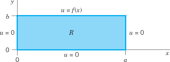
Fig. 296. Rectangle R and given boundary values
Dirichlet Problem in a Rectangle R (Fig. 296). We consider a Dirichlet problem for Laplace's equation (14) in a rectangle R, assuming that the temperature u(x, y) equals a given function f(x) on the upper side and 0 on the other three sides of the rectangle.
We solve this problem by separating variables. Substituting into u(x, y) = F(x)G(y) into (14) written as uxx = −uyy, dividing by FG, and equating both sides to a negative constant, we obtain

From this we get

and the left and right boundary conditions imply
![]()
This gives k = (nπ/a)2 and corresponding nonzero solutions
![]()
The ODE for G with k = (nπ/a)2 then becomes

Solutions are
![]()
Now the boundary condition u = 0 on the lower side of R implies that Gn(0) = 0; that is, Gn(0) = An + Bn = 0 or Bn = −An. This gives

From this and (15), writing ![]() , we obtain as the eigenfunctions of our problem
, we obtain as the eigenfunctions of our problem
![]()
These solutions satisfy the boundary condition u = 0 on the left, right, and lower sides.
To get a solution also satisfying the boundary condition u(x, b) = f(x) on the upper side, we consider the infinite series

From this and (16) with y = b we obtain
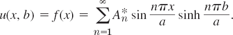
We can write this in the form

This shows that the expressions in the parentheses must be the Fourier coefficients bn of f(x); that is, by (4) in Sec. 11.3,

From this and (16) we see that the solution of our problem is

where

We have obtained this solution formally, neither considering convergence nor showing that the series for u, uxx and uyy have the right sums. This can be proved if one assumes that f and f′ are continuous and f″ is piecewise continuous on the interval 0 ![]() x
x ![]() a. The proof is somewhat involved and relies on uniform convergence. It can be found in [C4] listed in App. 1.
a. The proof is somewhat involved and relies on uniform convergence. It can be found in [C4] listed in App. 1.
Unifying Power of Methods. Electrostatics, Elasticity
The Laplace equation (14) also governs the electrostatic potential of electrical charges in any region that is free of these charges. Thus our steady-state heat problem can also be interpreted as an electrostatic potential problem. Then (17), (18) is the potential in the rectangle R when the upper side of R is at potential f(x) and the other three sides are grounded.
Actually, in the steady-state case, the two-dimensional wave equation (to be considered in Secs. 12.8, 12.9) also reduces to (14). Then (17), (18) is the displacement of a rectangular elastic membrane (rubber sheet, drumhead) that is fixed along its boundary, with three sides lying in the xy-plane and the fourth side given the displacement f(x).
This is another impressive demonstration of the unifying power of mathematics. It illustrates that entirely different physical systems may have the same mathematical model and can thus be treated by the same mathematical methods.
- Decay. How does the rate of decay of (8) with fixed n depend on the specific heat, the density, and the thermal conductivity of the material?
- Decay. If the first eigenfunction (8) of the bar decreases to half its value within 20 sec, what is the value of the diffusivity?
- Eigenfunctions. Sketch or graph and compare the first three eigenfunctions (8) with Bn = 1, c = 1, and L = π for t = 0, 0.1, 0.2, …, 1.0.
- WRITING PROJECT. Wave and Heat Equations. Compare these PDEs with respect to general behavior of eigenfunctions and kind of boundary and initial conditions. State the difference between Fig. 291 in Sec. 12.3 and Fig. 295.
5.7 LATERALLY INSULATED BAR
Find the temperature u(x, t) in a bar of silver of length 10 cm and constant cross section of area 1 cm2 (density 10.6 g/cm3, thermal conductivity 1.04 cal/(cm sec °C), specific heat 0.056 cal/(g °C) that is perfectly insulated laterally, with ends kept at temperature 0°C and initial temperature f(x) °C, where
- 5. f(x) = sin 0.1πx
- 6. f(x) = 4 − 0.8|x − 5|
- 7. f(x) = x(10 − x)
- 8. Arbitrary temperatures at ends. If the ends x = 0 and x = L of the bar in the text are kept at constant temperatures U1 and U, respectively, what is the temperature u1(x) in the bar after a long time (theoretically, as t → ∞)? First guess, then calculate.
- 9. In Prob. 8 find the temperature at any time.
- 10. Change of end temperatures. Assume that the ends of the bar in Probs. 5–7 have been kept at 100°C for a long time. Then at some instant, call it t = 0, the temperature at x = L is suddenly changed to 0°C and kept at 0°C, whereas the temperature at x = 0 is kept at 100°C. Find the temperature in the middle of the bar t = 1, 2, 3, 10, 50 sec. First guess, then calculate.
BAR UNDER ADIABATIC CONDITIONS
“Adiabatic” means no heat exchange with the neighborhood, because the bar is completely insulated, also at the ends. Physical Information: The heat flux at the ends is proportional to the value of ∂/∂x there.
- 11. Show that for the completely insulated bar, ux(0, t) = 0, ux(L, t) = 0, u(x, t) = f(x) and separation of variables gives the following solution, with An given by (2) in Sec. 11.3.
[12..15] Find the temperature in Prob. 11 with L = π, c = 1, and
- 12. f(x) = x
- 13. f(x) = 1
- 14. f(x) = cos 2x
- 15. f(x) = 1 − x/π
- 16. A bar with heat generation of constant rate H (> 0) is modeled by ut = c2uxx + H. Solve this problem if L = π and the ends of the bar are kept at 0°C. Hint. Set u = v −Hx(x − π)/(2c2).
- 17. Heat flux. The heat flux of a solution u(x, t) across x = 0 is defined by φ(t) = −Kux(0, t). Find φ(t) for the solution (9). Explain the name. Is it physically understandable that φ goes to 0 as t → ∞?
18.25 TWO-DIMENSIONAL PROBLEMS
- 18. Laplace equation. Find the potential in the rectangle 0 x 20, 0 y 40 whose upper side is kept at potential 110 V and whose other sides are grounded.
- 19. Find the potential in the square 0 x 2, 0 y 2 if the upper side is kept at the potential
 and the other sides are grounded.
 - 20. CAS PROJECT. Isotherms. Find the steady-state solutions (temperatures) in the square plate in Fig. 297 with a = 2 satisfying the following boundary conditions. Graph isotherms.
- u = 80 sin πx on the upper side, 0 on the others.
- u = 0 on the vertical sides, assuming that the other sides are perfectly insulated.
- Boundary conditions of your choice (such that the solution is not identically zero).

- 21. Heat flow in a plate. The faces of the thin square plate in Fig. 297 with side a = 24 are perfectly insulated. The upper side is kept at 25°C and the other sides are kept at 0°C. Find the steady-state temperature u(x, y) in the plate.
- 22. Find the steady-state temperature in the plate in Prob. 21 if the lower side is kept at U0°C, the upper side at U1°C, and the other sides are kept at 0°C. Hint: Split into two problems in which the boundary temperature is 0 on three sides for each problem.
- 23. Mixed boundary value problem. Find the steady-state temperature in the plate in Prob. 21 with the upper and lower sides perfectly insulated, the left side kept at 0°C, and the right side kept at f(y)°C.
- 24. Radiation. Find steady-state temperatures in the rectangle in Fig. 296 with the upper and left sides perfectly insulated and the right side radiating into a medium at 0°C according to ux(a, y) + hu(a, y) = 0, h > 0 constant. (You will get many solutions since no condition on the lower side is given.)
- 25. Find formulas similar to (17), (18) for the temperature in the rectangle R of the text when the lower side of R is kept at temperature f(x) and the other sides are kept at 0°C.
12.7 Heat Equation: Modeling Very Long Bars. Solution by Fourier Integrals and Transforms
Our discussion of the heat equation
in the last section extends to bars of infinite length, which are good models of very long bars or wires (such as a wire of length, say, 300 ft). Then the role of Fourier series in the solution process will be taken by Fourier integrals (Sec. 11.7).
Let us illustrate the method by solving (1) for a bar that extends to infinity on both sides (and is laterally insulated as before). Then we do not have boundary conditions, but only the initial condition
![]()
where f(x) is the given initial temperature of the bar.
To solve this problem, we start as in the last section, substituting u(x, t) = F(x)G(t) into (1). This gives the two ODEs
![]()
and
![]()
Solutions are
![]()
respectively, where A and B are any constants. Hence a solution of (1) is
![]()
Here we had to choose the separation constant k negative, k = −p2, because positive values of k would lead to an increasing exponential function in (5), which has no physical meaning.
Use of Fourier Integrals
Any series of functions (5), found in the usual manner by taking p as multiples of a fixed number, would lead to a function that is periodic in x when t = 0. However, since f(x) in (2) is not assumed to be periodic, it is natural to use Fourier integrals instead of Fourier series. Also, A and B in (5) are arbitrary and we may regard them as functions of p, writing A = A(p) and B = B(P). Now, since the heat equation (1) is linear and homogeneous, the function
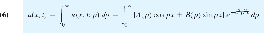
is then a solution of (1), provided this integral exists and can be differentiated twice with respect to x and once with respect to t.
Determination of A(p) and B(p) from the Initial Condition. From (6) and (2) we get

This gives A(p) and B(p) in terms of f(x); indeed, from (4) in Sec. 11.7 we have

According to (1*), Sec. 11.9, our Fourier integral (7) with these A(p) and B(p) can be written

Similarly, (6) in this section becomes
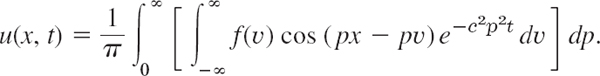
Assuming that we may reverse the order of integration, we obtain
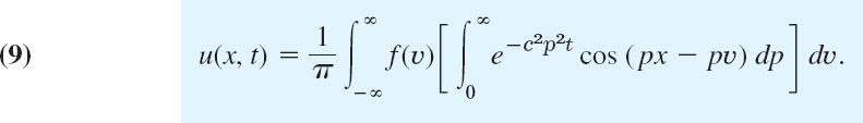
Then we can evaluate the inner integral by using the formula
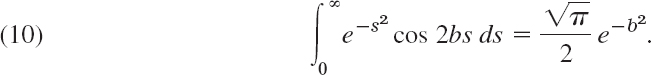
[A derivation of (10) is given in Problem Set 16.4 (Team Project 24).] This takes the form of our inner integral if we choose ![]() as a new variable of integration and set
as a new variable of integration and set

Then 2bs = (x − v)p and ![]() , so that (10) becomes
, so that (10) becomes
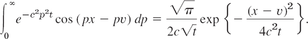
By inserting this result into (9) we obtain the representation

Taking ![]() as a variable of integration, we get the alternative form
as a variable of integration, we get the alternative form

If f(x) is bounded for all values of x and integrable in every finite interval, it can be shown (see Ref. [C10]) that the function (11) or (12) satisfies (1) and (2). Hence this function is the required solution in the present case.
EXAMPLE 1 Temperature in an Infinite Bar
Find the temperature in the infinite bar if the initial temperature is (Fig. 298)
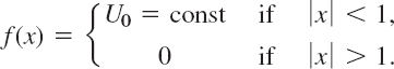
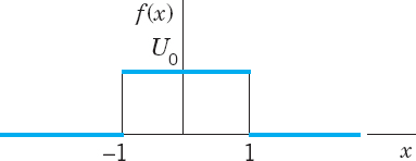
Fig. 298. Initial temperature in Example 1
Solution. From (11) we have

If we introduce the above variable of integration z, then the integration over v from −1 to 1 corresponds to the integration over z from ![]() to
to ![]() , and
, and

We mention that this integral is not an elementary function, but can be expressed in terms of the error function, whose values have been tabulated. (Table A4 in App. 5 contains a few values; larger tables are listed in Ref. [GenRef1] in App. 1. See also CAS Project 1, p. 574.) Figure 299 shows u(x, t) for U0 = 100°C, c2 = 1 cm2/sec, and several values of t.
Fig. 299. Solution u(x, t) in Example 1 for U0 = 100°C, c2 = 1 cm2/sec, and several values of t
Use of Fourier Transforms
The Fourier transform is closely related to the Fourier integral, from which we obtained the transform in Sec. 11.9. And the transition to the Fourier cosine and sine transform in Sec. 11.8 was even simpler. (You may perhaps wish to review this before going on.) Hence it should not surprise you that we can use these transforms for solving our present or similar problems. The Fourier transform applies to problems concerning the entire axis, and the Fourier cosine and sine transforms to problems involving the positive half-axis. Let us explain these transform methods by typical applications that fit our present discussion.
EXAMPLE 2 Temperature in the Infinite Bar in Example 1
Solve Example 1 using the Fourier transform.
Solution. The problem consists of the heat equation (1) and the initial condition (2), which in this example is
![]()
Our strategy is to take the Fourier transform with respect to x and then to solve the resulting ordinary DE in t. The details are as follows.
Let ![]() denote the Fourier transform of u, regarded as a function of x. From (10) in Sec. 11.9 we see that the heat equation (1) gives
denote the Fourier transform of u, regarded as a function of x. From (10) in Sec. 11.9 we see that the heat equation (1) gives
![]()
On the left, assuming that we may interchange the order of differentiation and integration, we have

Thus
Since this equation involves only a derivative with respect to t but none with respect to w, this is a first-order ordinary DE, with t as the independent variable and w as a parameter. By separating variables (Sec. 1.3) we get the general solution
![]()
with the arbitrary “constant” depending on the parameter w. The initial condition (2) yields the relationship ![]() . Our intermediate result is
. Our intermediate result is
![]()
The inversion formula (7), Sec. 11.9, now gives the solution

In this solution we may insert the Fourier transform

Assuming that we may invert the order of integration, we then obtain

By the Euler formula (3). Sec. 11.9, the integrand of the inner integral equals
![]()
We see that its imaginary part is an odd function of w, so that its integral is 0. (More precisely, this is the principal part of the integral; see Sec. 16.4.) The real part is an even function of w, so that its integral from −∞ to ∞ equals twice the integral from 0 to ∞:

This agrees with (9) (with p = w) and leads to the further formulas (11) and (13).
EXAMPLE 3 Solution in Example 1 by the Method of Convolution
Solve the heat problem in Example 1 by the method of convolution.
Solution. The beginning is as in Example 2 and leads to (14), that is,

Now comes the crucial idea. We recognize that this is of the form (13) in Sec. 11.9, that is,

where

Since, by the definition of convolution [(11), Sec. 11.9],

as our next and last step we must determine the inverse Fourier transform g of ![]() . For this we can use formula 9 in Table III of Sec. 11.10,
. For this we can use formula 9 in Table III of Sec. 11.10,

with a suitable a. With c2t = 1/(40a) or a = 1(4c2t) using (17) we obtain
![]()
Hence ![]() has the inverse
has the inverse

Replacing x with x − p and substituting this into (18) we finally have

This solution formula of our problem agrees with (11). We wrote (f * g)(x), without indicating the parameter t with respect to which we did not integrate.
EXAMPLE 4 Fourier Sine Transform Applied to the Heat Equation
If a laterally insulated bar extends from x = 0 to infinity, we can use the Fourier sine transform. We let the initial temperature be u(x, 0) = f(x) and impose the boundary condition u(0, t) = 0. Then from the heat equation and (9b) in Sec. 11.8, since f(0) = u(0,0) = 0, we obtain

This is a first-order ODE ∂ûs/∂t + c2w2ûs = 0. Its solution is
![]()
From the initial condition u(x, 0) = f(x) we have ûs(w, 0) = ![]() s(w) = C(w). Hence
s(w) = C(w). Hence
![]()
Taking the inverse Fourier sine transform and substituting

on the right, we obtain the solution formula

Figure 300 shows (20) with c = 1 for f(x) if 0 ![]() x
x ![]() 1 and 0 otherwise, graphed over the xt-plane for 0
1 and 0 otherwise, graphed over the xt-plane for 0 ![]() x
x ![]() 2, 0.01
2, 0.01 ![]() t
t ![]() 1.5. Note that the curves of u(x, t) for constant t resemble those in Fig. 299.
1.5. Note that the curves of u(x, t) for constant t resemble those in Fig. 299.

Fig. 300. Solution (20) in Example 4
- CAS PROJECT. Heat Flow.
- Graph the basic Fig. 299.
- In (a) apply animation to “see” the heat flow in terms of the decrease of temperature.
- Graph u(x, t) with c = 1 as a surface over a rectangle of the form −a < x < a, 0 < y < b.
2.8 SOLUTION IN INTEGRAL FORM
Using (6), obtain the solution of (1) in integral form satisfying the initial condition u(x, 0) = f(x) where
- 2. f(x) = 1 if|x| < a and 0 otherwise
- 3. f(x) = 1/(1 + x2). Hint. Use (15) in Sec. 11.7.
- 4. f(x) = e−|x|
- 5. f(x) = |x| if |x| < 1 and 0 otherwise
- 6. f(x) = x if |x| < 1 and 0 otherwise
- 7. f(x) = (sin x)/x. Hint. Use Prob. 4 in Sec. 11.7.
- 8. Verify that u in the solution of Prob. 7 satisfies the initial condition.
9.12 CAS PROJECT. Error Function.
This function is important in applied mathematics and physics (probability theory and statistics, thermodynamics, etc.) and fits our present discussion. Regarding it as a typical case of a special function defined by an integral that cannot be evaluated as in elementary calculus, do the following.
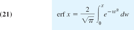
- 9. Graph the bell-shaped curve [the curve of the integrand in (21)]. Show that erf x is odd. Show that
- 10. Obtain the Maclaurin series of erf x from that of the integrand. Use that series to compute a table of erf x for (meaning x = 0, 0.01, 0.02, …, 3).
- 11. Obtain the values required in Prob. 10 by an integration command of your CAS. Compare accuracy.
- 12. It can be shown that erf(∞) = 1. Confirm this experimentally by computing erf x for large x.
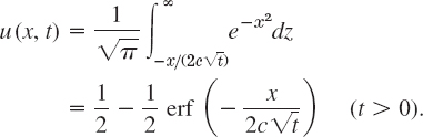
- 13. Let f(x) = 1 when x > 0 and 0 when x < 0. Using erf(∞) = 1, show that (12) then give
- 14. Express the temperature (13) in terms of the error function.
- 15. Show that
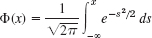
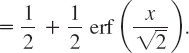
Here, the integral is the definition of the “distribution function of the normal probability distribution” to be discussed in Sec. 24.8.
12.8 Modeling: Membrane, Two-Dimensional Wave Equation
Since the modeling here will be similar to that of Sec. 12.2, you may want to take another look at Sec. 12.2.
The vibrating string in Sec. 12.2 is a basic one-dimensional vibrational problem. Equally important is its two-dimensional analog, namely, the motion of an elastic membrane, such as a drumhead, that is stretched and then fixed along its edge. Indeed, setting up the model will proceed almost as in Sec. 12.2.
Physical Assumptions
- The mass of the membrane per unit area is constant (“homogeneous membrane”). The membrane is perfectly flexible and offers no resistance to bending.
- The membrane is stretched and then fixed along its entire boundary in the xy-plane. The tension per unit length T caused by stretching the membrane is the same at all points and in all directions and does not change during the motion.
- The deflection u(x, y, t) of the membrane during the motion is small compared to the size of the membrane, and all angles of inclination are small.
Although these assumptions cannot be realized exactly, they hold relatively accurately for small transverse vibrations of a thin elastic membrane, so that we shall obtain a good model, for instance, of a drumhead.
Derivation of the PDE of the Model (“Two-Dimensional Wave Equation”) from Forces. As in Sec. 12.2 the model will consist of a PDE and additional conditions. The PDE will be obtained by the same method as in Sec. 12.2, namely, by considering the forces acting on a small portion of the physical system, the membrane in Fig. 301 on the next page, as it is moving up and down.
Since the deflections of the membrane and the angles of inclination are small, the sides of the portion are approximately equal to Δx and Δy. The tension T is the force per unit length. Hence the forces acting on the sides of the portion are approximately TΔx and TΔy. Since the membrane is perfectly flexible, these forces are tangent to the moving membrane at every instant.
Horizontal Components of the Forces. We first consider the horizontal components of the forces. These components are obtained by multiplying the forces by the cosines of the angles of inclination. Since these angles are small, their cosines are close to 1. Hence the horizontal components of the forces at opposite sides are approximately equal. Therefore, the motion of the particles of the membrane in a horizontal direction will be negligibly small. From this we conclude that we may regard the motion of the membrane as transversal; that is, each particle moves vertically.
Vertical Components of the Forces. These components along the right side and the left side are (Fig. 301), respectively,
![]()
Here α and β are the values of the angle of inclination (which varies slightly along the edges) in the middle of the edges, and the minus sign appears because the force on the left side is directed downward. Since the angles are small, we may replace their sines by their tangents. Hence the resultant of those two vertical components is
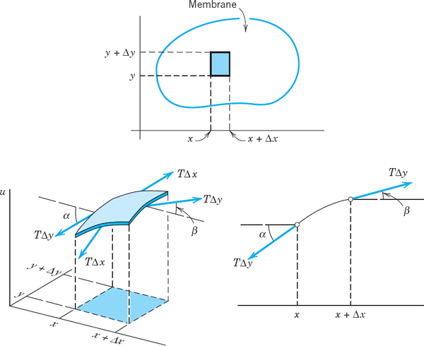

where subscripts x denote partial derivatives and y1 and y2 are values between y and y + Δy. Similarly, the resultant of the vertical components of the forces acting on the other two sides of the portion is
![]()
where x1 and x2 are values between x and x + Δx.
Newton's Second Law Gives the PDE of the Model. By Newton's second law (see Sec. 2.4) the sum of the forces given by (1) and (2) is equal to the mass ρΔA of that small portion times the acceleration ∂2u/∂2; here ρ is the mass of the undeflected membrane per unit area, and ΔA = Δx Δy is the area of that portion when it is undeflected. Thus

where the derivative on the left is evaluated at some suitable point ![]() corresponding to that portion. Division by ρΔxΔy gives
corresponding to that portion. Division by ρΔxΔy gives

If we let Δ0x and Δy approach zero, we obtain the PDE of the model

This PDE is called the two-dimensional wave equation. The expression in parentheses is the Laplacian Δ2u of u (Sec. 10.8). Hence (3) can be written

Solutions of the wave equation (3) will be obtained and discussed in the next section.
12.9 Rectangular Membrane. Double Fourier Series
Now we develop a solution for the PDE obtained in Sec. 12.8. Details are as follows.
The model of the vibrating membrane for obtaining the displacement u(x, y, t) of a point (x, y) of the membrane from rest (u = 0) at time t is
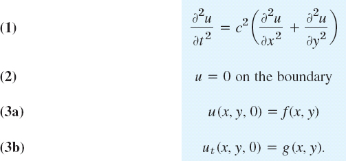
Here (1) is the two-dimensional wave equation with c2 = T/ρ just derived, (2) is the boundary condition (membrane fixed along the boundary in the xy-plane for all times t ![]() 0), and (3) are the initial conditions at t = 0, consisting of the given initial displacement (initial shape) f(x, y) and the given initial velocity g(x, y), where ut = ∂u/∂t. We see that these conditions are quite similar to those for the string in Sec. 12.2.
0), and (3) are the initial conditions at t = 0, consisting of the given initial displacement (initial shape) f(x, y) and the given initial velocity g(x, y), where ut = ∂u/∂t. We see that these conditions are quite similar to those for the string in Sec. 12.2.

Fig. 302. Rectangular membrane
Let us consider the rectangular membrane R in Fig. 302. This is our first important model. It is much simpler than the circular drumhead, which will follow later. First we note that the boundary in equation (2) is the rectangle in Fig. 302. We shall solve this problem in three steps:
Step 1. By separating variables, first setting u(x, y, t) = F(x, y)G(t) and later F(x, y) = H(x)Q(y) we obtain from (1) an ODE (4) for G and later from a PDE (5) for F two ODEs (6) and (7) for H and Q.
Step 2. From the solutions of those ODEs we determine solutions (13) of (1) (“eigenfunctions” umn) that satisfy the boundary condition (2).
Step 3. We compose the umn into a double series (14) solving the whole model (1), (2), (3).
Step 1. Three ODEs From the Wave Equation (1)
To obtain ODEs from (1), we apply two successive separations of variables. In the first separation we set u(x, y, t) = F(x, y)G(t). Substitution into (1) gives
![]()
where subscripts denote partial derivatives and dots denote derivatives with respect to t. To separate the variables, we divide both sides by c2FG:

Since the left side depends only on t, whereas the right side is independent of t, both sides must equal a constant. By a simple investigation we see that only negative values of that constant will lead to solutions that satisfy (2) without being identically zero; this is similar to Sec. 12.3. Denoting that negative constant by −v2, we have

This gives two equations: for the “time function” G(t) we have the ODE

and for the “amplitude function” F(x, y) a PDE, called the two-dimensional Helmholtz3 equation
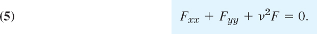
Separation of the Helmholtz equation is achieved if we set F(x, y) = H(x)Q(y). By substitution of this into (5) we obtain
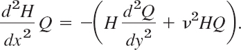
To separate the variables, we divide both sides by HQ, finding
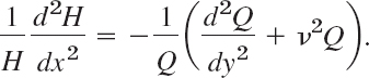
Both sides must equal a constant, by the usual argument. This constant must be negative, say, −k2, because only negative values will lead to solutions that satisfy (2) without being identically zero. Thus

This yields two ODEs for H and Q, namely,

and
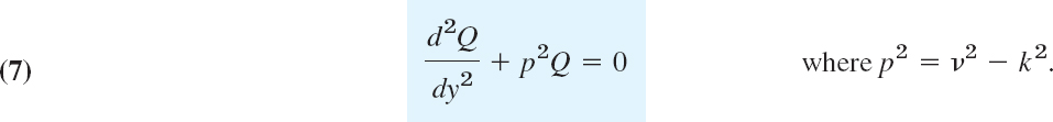
Step 2. Satisfying the Boundary Condition
General solutions of (6) and (7) are
![]()
with constant A, B, C, D. From u = FG and (2) it follows that F = HQ must be zero on the boundary, that is, on the edges x = 0, x = a, y = 0, y = b; see Fig. 302. This gives the conditions
![]()
Hence H(0) = A = 0 and then H(a) = B sin ka = 0. Here we must take B ≠ 0 since otherwise H(x) ≡ 0 and F(x, y) ≡ 0. Hence sin ka = 0 or ka = mπ, that is,
![]()
In precisely the same fashion we conclude that c = 0 and p must be restricted to the values p = nπ/b where n is an integer. We thus obtain the solutions H = Hm, Q = Qn, where
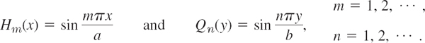
As in the case of the vibrating string, it is not necessary to consider m, n = −1, −2, … since the corresponding solutions are essentially the same as for positive m and n, expect for a factor −1. Hence the functions

are solutions of the Helmholtz equation (5) that are zero on the boundary of our membrane.
Eigenfunctions and Eigenvalues. Having taken care of (5), we turn to (4). Since p2 = v2 − k2 in (7) and λ = cv in (4), we have
![]()
Hence to k = mπ/a and p = nπ/b there corresponds the value

in the ODE (4). A corresponding general solution of (4) is
![]()
It follows that the functions umn(x, y, t) = Fmn(x, y)Gmn(t), written out

with λmn according to (9), are solutions of the wave equation (1) that are zero on the boundary of the rectangular membrane in Fig. 302. These functions are called the eigenfunctions or characteristic functions, and the numbers λmn are called the eigenvalues or characteristic values of the vibrating membrane. The frequency of umn is λmn/2π.
Discussion of Eigenfunctions. It is very interesting that, depending on a and b, several functions Fmn may correspond to the same eigenvalue. Physically this means that there may exists vibrations having the same frequency but entirely different nodal lines (curves of points on the membrane that do not move). Let us illustrate this with the following example.
EXAMPLE 1 Eigenvalues and Eigenfunctions of the Square Membrane
Consider the square membrane with a = b = 1. From (9) we obtain its eigenvalues
![]()
Hence λmn = λnm, but for m ≠ n the corresponding functions
![]()
are certainly different. For example, to λ12 = λ21 = ![]() there correspond the two functions
there correspond the two functions
![]()
Hence the corresponding solutions
![]()
have the nodal lines ![]() , and respectively (see Fig. 303). Taking B12 = 1 and
, and respectively (see Fig. 303). Taking B12 = 1 and ![]() , we obtain
, we obtain
![]()
which represents another vibration corresponding to the eigenvalue ![]() . The nodal line of this function is the solution of the equation
. The nodal line of this function is the solution of the equation
![]()
or, since sin 2α = 2 sin α cos α,
![]()
This solution depends on the value of B21 (see Fig. 304).
From (11) we see that even more than two functions may correspond to the same numerical value of λmn. For example, the four functions F18, F81, F47, and F74 correspond to the value
![]()
This happens because 65 can be expressed as the sum of two squares of positive integers in several ways. According to a theorem by Gauss, this is the case for every sum of two squares among whose prime factors there are at least two different ones of the form 4n + 1 where n is a positive integer. In our case we have 65 = 5 · 13 = (4 + 1)(12 + 1).

Fig. 303. Nodal lines of the solutions u11, u12, u21, u22, u13, u31 in the case of the square membrane
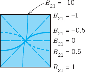
Fig. 304. Nodal lines of the solution (12) for some values of B21
Step 3. Solution of the Model (1), (2), (3). Double Fourier Series
So far we have solutions (10) satisfying (1) and (2) only. To obtain the solutions that also satisfies (3), we proceed as in Sec. 12.3. We consider the double series

(without discussing convergence and uniqueness). From (14) and (3a), setting we have
Suppose that f(x, y) can be represented by (15). (Sufficient for this is the continuity of f, ∂f/∂x, ∂f/∂y, ∂2f/∂x ∂y in R.) Then (15) is called the double Fourier series of f(x, y). Its coefficients can be determined as follows. Setting

we can write (15) in the form
For fixed y this is the Fourier sine series of f(x, y) considered as a function of x. From (4) in Sec. 11.3 we see that the coefficients of this expansion are

Furthermore, (16) is the Fourier sine series of Km(y), and from (4) in Sec. 11.3 it follows that the coefficients are
From this and (17) we obtain the generalized Euler formula

for the Fourier coefficients of f(x, y) in the double Fourier series (15).
The Bmn in (14) are now determined in terms of f(x, y). To determine the ![]() , we differentiate (14) termwise with respect to t; using (3b), we obtain
, we differentiate (14) termwise with respect to t; using (3b), we obtain
Suppose that g(x, y) can be developed in this double Fourier series. Then, proceeding as before, we find that the coefficients are
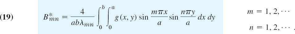
Result. If f and g in (3) are such that u can be represented by (14), then (14) with coefficients (18) and (19) is the solution of the model (1), (2), (3).
EXAMPLE 2 Vibration of a Rectangular Membrane
Find the vibrations of a rectangular membrane of sides a = 4 ft and b = 2 ft (Fig. 305) if the tension is 12.5 lb/ft, the density is 2.5 slugs/ft2 (as for light rubber), the initial velocity is 0, and the initial displacement is
![]()
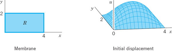
Fig. 305. Example 2
Solution. c2 = T/ρ = 12.5/2.5 = 5[ft2/sec2]. Also ![]() from (19). From (18) and (20),
from (19). From (18) and (20),

Two integrations by parts give for the first integral on the right

and for the second integral

For even m or n we get 0. Together with the factor 1/20 we thus have Bmn = 0 if m or n is even and

From this, (9), and (14) we obtain the answer

To discuss this solution, we note that the first term is very similar to the initial shape of the membrane, has no nodal lines, and is by far the dominating term because the coefficients of the next terms are much smaller. The second term has two horizontal nodal lines ![]() , the third term two vertical ones
, the third term two vertical ones ![]() , the fourth term two horizontal and two vertical ones, and so on.
, the fourth term two horizontal and two vertical ones, and so on.
- Frequency. How does the frequency of the eigenfunctions of the rectangular membrane change (a) If we double the tension? (b) If we take a membrane of half the density of the original one? (c) If we double the sides of the membrane? Give reasons.
- Assumptions. Which part of Assumption 2 cannot be satisfied exactly? Why did we also assume that the angles of inclination are small?
- Determine and sketch the nodal lines of the square membrane for m = 1, 2, 3, 4 and n = 1, 2, 3, 4.
4.8 DOUBLE FOURIER SERIES
Represent f(x, y) by a series (15), where
- 4. f(x, y) = 1, a = b = 1
- 5. f(x, y) = y, a = b = 1
- 6. f(x, y) = x, a = b = 1
- 7. f(x, y) = xy, a and b arbitrary
- 8. f(x, y) = xy(a − x)(b − y), a and b arbitrary
- 9. CAS PROJECT. Double Fourier Series.
- Write a program that gives and graphs partial sums of (15). Apply it to Probs. 5 and 6. Do the graphs show that those partial sums satisfy the boundary condition (3a)? Explain why. Why is the convergence rapid?
- Do the tasks in (a) for Prob. 4. Graph a portion, say,
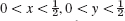 , of several partial sums on common axes, so that you can see how they differ. (See Fig. 306.)
 - Do the tasks in (b) for functions of your choice.

- 10. CAS EXPERIMENT. Quadruples of Fmn. Write a program that gives you four numerically equal λmn in Example 1, so that four different Fmn correspond to it. Sketch the nodal lines of F18, F81, F74 in Example 1 and similarly for further Fmn that you will find.
11.13 SQUARE MEMBRANE
Find the deflection u(x, y, t) of the square membrane of side π and c2 = 1 for initial velocity 0 and initial deflection
- 11. 0.1 sin 2x sin 4y
- 12. 0.01 sin x sin y
- 13. 0.1xy(π − x)(π − y)
- 14. Verify the discussion of (21) in Example 2.
- 15. Do Prob. 3 for the membrane with a = 4 and b = 2.
- 16. Verify Bmn in Example 2 by integration by parts.
- 17. Find eigenvalues of the rectangular membrane of sides a = 2 and b = 1 to which there correspond two or more different (independent) eigenfunctions.
- 18. Minimum property. Show that among all rectangular membranes of the same area A = ab and the same c the square membrane is that for which [see (10)] has the lowest frequency.
- 19. Deflection. Find the deflection of the membrane of sides a and b with c2 = 1 for the initial deflection
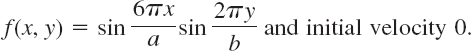
- 20. Forced vibrations. Show that forced vibrations of a membrane are modeled by the
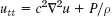 where P(x, y, t) is the external force per unit area acting perpendicular to the xy-plane.
12.10 Laplacian in Polar Coordinates. Circular Membrane. Fourier–Bessel Series
It is a general principle in boundary value problems for PDEs to choose coordinates that make the formula for the boundary as simple as possible. Here polar coordinates are used for this purpose as follows. Since we want to discuss circular membranes (drumheads), we first transform the Laplacian in the wave equation (1), Sec. 12.9,
![]()
(subscripts denoting partial derivatives) into polar coordinates r, θ defined by x = r cos θ, y = r sin θ;, thus

By the chain rule (Sec. 9.6) we obtain
![]()
Differentiating once more with respect to x and using the product rule and then again the chain rule gives
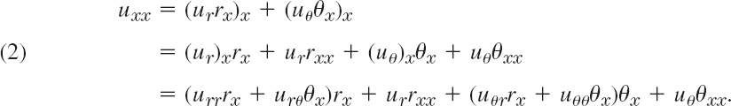
Also, by differentiation of r and θ we find
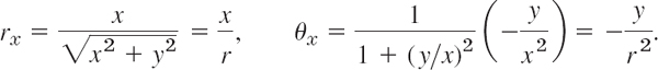
Differentiating these two formulas again, we obtain

We substitute all these expressions into (2). Assuming continuity of the first and second partial derivatives, we have urθ = uθr, and by simplifying,

In a similar fashion it follows that

By adding (3) and (4) we see that the Laplacian of u in polar coordinates is
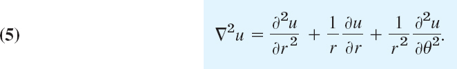
Circular Membrane
Circular membranes are important parts of drums, pumps, microphones, telephones, and other devices. This accounts for their great importance in engineering. Whenever a circular membrane is plane and its material is elastic, but offers no resistance to bending (this excludes thin metallic membranes!), its vibrations are modeled by the two-dimensional wave equation in polar coordinates obtained from (1) with ![]() given by (5), that is,
given by (5), that is,
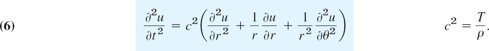
We shall consider a membrane of radius R (Fig. 307) and determine solutions u(r, t) that are radially symmetric. (Solutions also depending on the angle θ will be discussed in the problem set.) Then uθθ = 0 in (6) and the model of the problem (the analog of (1), (2), (3) in Sec. 12.9) is
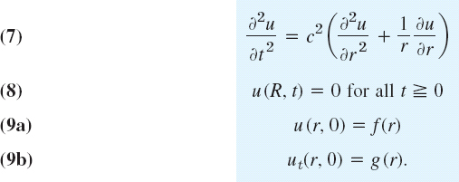

Here (8) means that the membrane is fixed along the boundary circle r = R. The initial deflection f(r) and the initial velocity g(r) depend only on r, not on θ, so that we can expect radially symmetric solutions u(r, t).
Step 1. Two ODEs From the Wave Equation (7). Bessel's Equation
Using the method of separation of variables, we first determine solutions u(r, t) = W(r)G(t). (We write W, not F because W depends on r, whereas F, used before, depended on x.) Substituting u = WG and its derivatives into (7) and dividing the result by c2WG we get
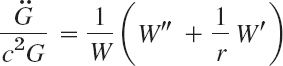
where dots denote derivatives with respect to t and primes denote derivatives with respect to r. The expressions on both sides must equal a constant. This constant must be negative, say, −k2, in order to obtain solutions that satisfy the boundary condition without being identically zero. Thus,

This gives the two linear ODEs

and
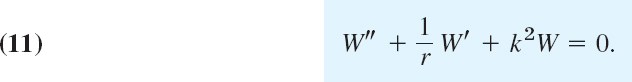
We can reduce (11) to Bessel's equation (Sec. 5.4) if we set s = kr. Then 1/r = k/s and, retaining the notation W for simplicity, we obtain by the chain rule

By substituting this into (11) and omitting the common factor k2 we have

This is Bessel's equation (1), Sec. 5.4, with parameter v = 0.
Step 2. Satisfying the Boundary Condition (8)
Solutions of (12) are the Bessel functions J0 and Y0 of the first and second kind (see Secs. 5.4, 5.5). But Y0 becomes infinite at 0, so that we cannot use it because the deflection of the membrane must always remain finite. This leaves us with
![]()
On the boundary r = R we get W(R) = J0(kR) = 0 from (8) (because G ≡ 0 would imply u ≡ 0). We can satisfy this condition because J0 has (infinitely many) positive zeros, s = α1, α2, … (see Fig. 308), with numerical values
![]()
and so on. (For further values, consult your CAS or Ref. [GenRef1] in App. 1.) These zeros are slightly irregularly spaced, as we see. Equation (13) now implies

Hence the functions

are solutions of (11) that are zero on the boundary circle r = R.
Eigenfunctions and Eigenvalues. For Wm in (15), a corresponding general solution of (10) with λ = λm = ckm = cαm/R is
![]()
Hence the functions

with m = 1, 2, … are solutions of the wave equation (7) satisfying the boundary condition (8). These are the eigenfunctions of our problem. The corresponding eigenvalues are λm.
The vibration of the membrane corresponding to um is called the mth normal mode; it has the frequency λm/2π cycles per unit time. Since the zeros of the Bessel function are not regularly spaced on the axis (in contrast to the zeros of the sine functions appearing in the case of the vibrating string), the sound of a drum is entirely different from that of a violin. The forms of the normal modes can easily be obtained from Fig. 308 and are shown in Fig. 309. For m = 1, all the points of the membrane move up (or down) at the same time. For m = 2, the situation is as follows. The function W2(r) = J0(α2r/R) is zero for α2r/R = α1, thus r = α1R/α2. The circle r = α1R/α2 is, therefore, nodal line, and when at some instant the central part of the membrane moves up, the outer part (r > α1R/α2) moves down, and conversely. The solution um(r, t) has m − 1 nodal lines, which are circles (Fig. 309).
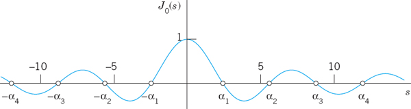
Fig. 308. Bessel function J0(s)

Fig. 309. Normal modes of the circular membrane in the case of vibrations independent of the angle
Step 3. Solution of the Entire Problem
To obtain a solution u(r, t) that also satisfies the initial conditions (9), we may proceed as in the case of the string. That is, we consider the series
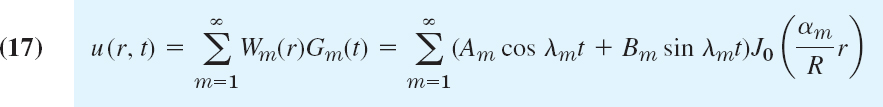
(leaving aside the problems of convergence and uniqueness). Setting t = 0 and using (9a), we obtain

Thus for the series (17) to satisfy the condition (9a), the constants Am must be the coefficients of the Fourier–Bessel series (18) that represents f(r) in terms of J0(αmr/R) that is [see (9) in Sec. 11.6 with n = 0, α0, m = αm and x = r],

Differentiability of f(r) in the interval 0 ![]() r
r ![]() R is sufficient for the existence of the development (18); see Ref. [A13]. The coefficients Bm in (17) can be determined from (9b) in a similar fashion. Numeric values of Am and Bm may be obtained from a CAS or by a numeric integration method, using tables of J0 and J1. However, numeric integration can sometimes be avoided, as the following example shows.
R is sufficient for the existence of the development (18); see Ref. [A13]. The coefficients Bm in (17) can be determined from (9b) in a similar fashion. Numeric values of Am and Bm may be obtained from a CAS or by a numeric integration method, using tables of J0 and J1. However, numeric integration can sometimes be avoided, as the following example shows.
EXAMPLE 1 Vibrations of a Circular Membrane
Find the vibrations of a circular drumhead of radius 1 ft and density 2 slugs/ft2 if the tension is 8 lb/ft, the initial velocity is 0, and the initial displacement is
![]()
Solution. ![]() . Also Bm = 0, since the initial velocity is 0. From (10) in Sec. 11.6, since R = 1, we obtain
. Also Bm = 0, since the initial velocity is 0. From (10) in Sec. 11.6, since R = 1, we obtain

where the last equality follows from (21c), Sec. 5.4, with v = 1, that is,

Table 9.5 on p. 409 of [GenRef1] gives am and ![]() . From this we get
. From this we get ![]() by (21b), Sec. 5.4, with v = 0, and compute the coefficients Am:
by (21b), Sec. 5.4, with v = 0, and compute the coefficients Am:
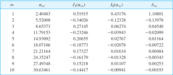
Thus
![]()
We see that the coefficients decrease relatively slowly. The sum of the explicitly given coefficients in the table is 0.99915. The sum of all the coefficients should be 1. (Why?) Hence by the Leibniz test in App. A3.3 the partial sum of those terms gives about three correct decimals of the amplitude f(r).
Since
![]()
from (17) we thus obtain the solution (with r measured in feet and t in seconds)
![]()
In Fig. 309, m = 1 gives an idea of the motion of the first term of our series, m = 2 of the second term, and m = 3 of the third term, so that we can “see” our result about as well as for a violin string in Sec. 12.3.
1.3 RADIAL SYMMETRY
- Why did we introduce polar coordinates in this section?
- Radial symmetry reduces (5) to
 . Derive this directly from
  . Show that the only solution of
  depending only on
  is u = a ln r + b with arbitrary constants a and b.
 - Alternative form of (5). Show that (5) can be written
 , a form that is often practical.
BOUNDARY VALUE PROBLEMS. SERIES
- 4. TEAM PROJECT. Series for Dirichlet and Neumann Problems
- Show that un = rncos nθ, un = rn sin nθ, n = 0, 1, …, are solutions of Laplace's equation
 with
with  given by (5). (What would un be in Cartesian coordinates? Experiment with small n.)
 - Dirichlet problem (See Sec. 12.6) Assuming that termwise differentiation is permissible, show that a solution of the Laplace equation in the disk r < R satisfying the boundary condition u(R, θ) = f(θ) and (R and f given) is

where an, bn are the Fourier coefficients of f (see Sec. 11.1).
- Dirichlet problem. Solve the Dirichlet problem using (20) if R = 1 and the boundary values are u(θ) = −100 volts if −π < θ < 0, u(θ) volts if 0 < θ < π. (Sketch this disk, indicate the boundary values.)
- Neumann problem. Show that the solution of the Neumann problem
 if r < R, uN(R, θ) = f(θ) (where uN = ∂u/∂N is the directional derivative in the direction of the outer normal) is
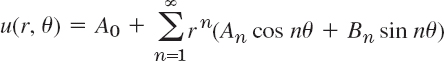
with arbitary A0 and
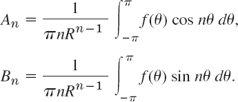
- Compatibility condition. Show that (9), Sec. 10.4, imposes on in f(θ) in (d) the “compatibility condition”

- Neumann problem. Solve
 in the annulus 1 < r < 2 if ur(1, θ) = sin θ, ur(2, θ) = 0.
- Show that un = rncos nθ, un = rn sin nθ, n = 0, 1, …, are solutions of Laplace's equation
5.8 ELECTROSTATIC POTENTIAL. STEADY-STATE HEAT PROBLEMS
The electrostatic potential satisfies Laplace's equation ![]() in any region free of charges. Also the heat equation
in any region free of charges. Also the heat equation ![]() (Sec. 12.5) reduces to Laplace's equation if the temperature u is time-independent (“steady-state case”). Using (20), find the potential (equivalently: the steady-state temperature) in the disk r < 1 if the boundary values are (sketch them, to see what is going on).
(Sec. 12.5) reduces to Laplace's equation if the temperature u is time-independent (“steady-state case”). Using (20), find the potential (equivalently: the steady-state temperature) in the disk r < 1 if the boundary values are (sketch them, to see what is going on).
- 5. u(1, θ) = 220
 and 0 otherwise
 - 6. u(1, θ) = 400 cos3θ
- 7. u(1, θ) = 110|θ| if −π < θ < π
- 8. u(1, θ) = θ
 and 0 otherwise
 - 9. CAS EXPERIMENT. Equipotential Lines. Guess what the equipotential lines u(r, θ) = const in Probs. 5 and 7 may look like. Then graph some of them, using partial sums of the series.
- 10. Semidisk. Find the electrostatic potential in the semi-disk r < 1, 0 < θ < π which equals 110θ(π − θ) on the semicircle r = 1 and 0 on the segment −1 < x < 1.
- 11. Semidisk. Find the steady-state temperature in a semicircular thin plate r < a, 0 < θ < π with the semicircle r = a kept at constant temperature u0 and the segment −a < x < a at 0.
CIRCULAR MEMBRANE
- 12. CAS PROJECT. Normal Modes.
- Graph the normal modes as in Fig. 306. u4, u5, u6 as in Fig. 306.
- Write a program for calculating the Am's in Example 1 and extend the table to m = 15. Verify numerically that
 and compute the error for m = 1, …, 10.
 - Graph the initial deflection f(r) in Example 1 as well as the first three partial sums of the series. Comment on accuracy.
- Compute the radii of the nodal lines of u2, u3, u4 when R = 1. How do these values compare to those of the nodes of the vibrating string of length 1? Can you establish any empirical laws by experimentation with further um?
- 13. Frequency. What happens to the frequency of an eigenfunction of a drum if you double the tension?
- 14. Size of a drum. A small drum should have a higher fundamental frequency than a large one, tension and density being the same. How does this follow from our formulas?
- 15. Tension. Find a formula for the tension required to produce a desired fundamental frequency f1 of a drum.
- 16. Why is A1 + A2 + … = 1 in Example 1? Compute the first few partial sums until you get 3-digit accuracy. What does this problem mean in the field of music?
- 17. Nodal lines. Is it possible that for fixed c and R two or more um [see (16)] with different nodal lines correspond to the same eigenvalue? (Give a reason.)
- 18. Nonzero initial velocity is more of theoretical interest because it is difficult to obtain experimentally. Show that for (17) to satisfy (9b) we must have

where

VIBRATIONS OF A CIRCULAR MEMBRANE DEPENDING ON BOTH r AND θ
- 19. (Separations) Show that substitution of u = F(r, θ)G(t) into the wave equation (6), that is,

gives an ODE and a PDE

Show that the PDE can now be separated by substituting F = W(r)Q(θ), giving


- 20 Periodicity. Show that Q(θ) must be periodic with period 2π and, therefore, n = 0, 1, 2, … in (25) and (26). Show that this yields the solutions Qn = cos nθ,
 , Wn = Jn(kr), n = 0, 1, ….
 - 21. Boundary condition. Show that the boundary condition

leads to k = kmn = αmn/R, where s = αnm is the mth positive zero of Jn(s).
- 22. Solutions depending on both r and θ. Show that solutions of (22) satisfying (27) are (see Fig. 310)


- 23. Initial condition. Show that ut(r, θ, 0) = 0 gives Bnm = 0,
 = 0 in (28).
 - 24. Show that
 and u0m is identical with (16) in this section.
 - 25. Semicircular membrane. Show that u11 represents the fundamental mode of a semicircular membrane and find the corresponding frequency when c2 = 1 and R = 1.
12.11 Laplace's Equation in Cylindrical and Spherical Coordinates. Potential
One of the most important PDEs in physics and engineering applications is Laplace's equation, given by
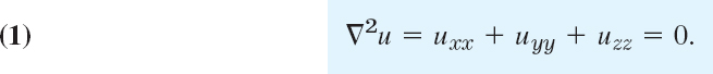
Here, x, y, z are Cartesian coordinates in space (Fig. 167 in Sec. 9.1), etc. uxx = ∂2u = ∂x2, etc. The expression ![]() is called the Laplacian of u. The theory of the solutions of (1) is called potential theory. Solutions of (1) that have continuous second partial derivatives are known as harmonic functions.
is called the Laplacian of u. The theory of the solutions of (1) is called potential theory. Solutions of (1) that have continuous second partial derivatives are known as harmonic functions.
Laplace's equation occurs mainly in gravitation, electrostatics (see Theorem 3, Sec. 9.7), steady-state heat flow (Sec. 12.5), and fluid flow (to be discussed in Sec. 18.4).
Recall from Sec. 9.7 that the gravitational potential u(x, y, z) at a point (x, y, z) resulting from a single mass located at a point (X, Y, Z) is

and u satisfies (1). Similarly, if mass is distributed in a region T in space with density ρ(X, Y, Z), its potential at a point (x, y, z) not occupied by mass is

It satisfies (1) because ![]() (Sec. 9.7) and ρ is not a function of x, y, z.
(Sec. 9.7) and ρ is not a function of x, y, z.
Practical problems involving Laplace's equation are boundary value problems in a region T in space with boundary surface S. Such problems can be grouped into three types (see also Sec. 12.6 for the two-dimensional case):
- First boundary value problem or Dirichlet problem if u is prescribed on S.
- Second boundary value problem or Neumann problem if the normal derivative un = ∂u/∂n is prescribed on S.
- Third or mixed boundary value problem or Robin problem if u is prescribed on a portion of S and un on the remaining portion of S.
In general, when we want to solve a boundary value problem, we have to first select the appropriate coordinates in which the boundary surface S has a simple representation. Here are some examples followed by some applications.
Laplacian in Cylindrical Coordinates
The first step in solving a boundary value problem is generally the introduction of coordinates in which the boundary surface S has a simple representation. Cylindrical symmetry (a cylinder as a region T) calls for cylindrical coordinates r, θ, z related to x, y, z by
![]()

Fig. 311. Cylindrical coordinates (r ![]() 0, 0
0, 0 ![]() θ
θ ![]() 2π)
2π)
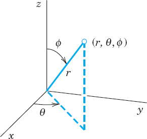
Fig. 312. Spherical coordinates (r ![]() 0, 0
0, 0 ![]() θ
θ ![]() 2π, 0
2π, 0 ![]() φ
φ ![]() π)
π)
For these we get ![]() immediately by adding uzz to (5) in Sec. 12.10; thus,
immediately by adding uzz to (5) in Sec. 12.10; thus,

Laplacian in Spherical Coordinates
Spherical symmetry (a ball as region T bounded by a sphere S) requires spherical coordinates r, θ, φ related to x, y, z by
![]()
Using the chain rule (as in Sec. 12.10), we obtain ![]() in spherical coordinates
in spherical coordinates

We leave the details as an exercise. It is sometimes practical to write (7) in the form

Remark on Notation. Equation (6) is used in calculus and extends the familiar notation for polar coordinates. Unfortunately, some books use θ and φ interchanged, an extension of the notation x = r cos φ, y = r sin φ for polar coordinates (used in some European countries).
Boundary Value Problem in Spherical Coordinates
We shall solve the following Dirichlet problem in spherical coordinates:
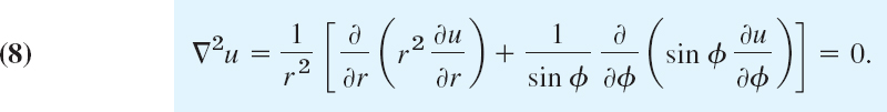
![]()
![]()
The PDE (8) follows from (7) or (7′) by assuming that the solution u will not depend on because the Dirichlet condition (9) is independent of θ. This may be an electrostatic potential (or a temperature) f(φ) at which the sphere S: r = R is kept. Condition (10) means that the potential at infinity will be zero.
Separating Variables by substituting u(r, φ) = G(r)H(φ) into (8). Multiplying (8) by r2, making the substitution and then dividing by GH, we obtain

By the usual argument both sides must be equal to a constant k. Thus we get the two ODEs

and

The solutions of (11) will take a simple form if we set k = n(n + 1). Then, writing G′ = dG/dr, etc., we obtain
![]()
This is an Euler–Cauchy equation. From Sec. 2.5 we know that it has solutions G = ra. Substituting this and dropping the common factor ra gives
![]()
Hence solutions are

We now solve (12). Setting cos φ = w we have sin2φ = 1 − w2 and

Consequently, (12) with k = n(n + 1) takes the form

This is Legendre's equation (see Sec. 5.3), written out
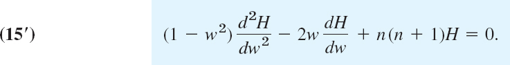
For integer n = 0, 1, … the Legendre polynomials
![]()
are solutions of Legendre's equation (15). We thus obtain the following two sequences of solution u = GH of Laplace's equation (8), with constant An and Bn, where n = 0, 1, …,

Use of Fourier–Legendre Series
Interior Problem: Potential Within the Sphere S. We consider a series of terms from (16a),

Since S is given by r = R for (17) to satisfy the Dirichlet condition (9) on the sphere S, we must have

that is, (18) must be the Fourier–Legendre series of f(φ). From (7) in Sec. 5.8 we get the coefficients

where ![]() denotes f(φ) as a function of w = cosφ. Since dw = −sin φ dφ, and the limits of integration and −1 correspond to φ = π and φ = 0, respectively, we also obtain
denotes f(φ) as a function of w = cosφ. Since dw = −sin φ dφ, and the limits of integration and −1 correspond to φ = π and φ = 0, respectively, we also obtain
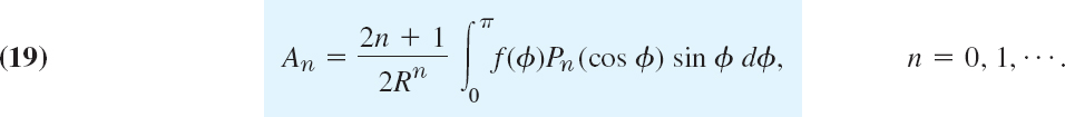
If f(φ) and f′(φ) are piecewise continuous on the interval 0 ![]() φ
φ ![]() π, then the series (17) with coefficients (19) solves our problem for points inside the sphere because it can be shown that under these continuity assumptions the series (17) with coefficients (19) gives the derivatives occurring in (8) by termwise differentiation, thus justifying our derivation.
π, then the series (17) with coefficients (19) solves our problem for points inside the sphere because it can be shown that under these continuity assumptions the series (17) with coefficients (19) gives the derivatives occurring in (8) by termwise differentiation, thus justifying our derivation.
Exterior Problem: Potential Outside the Sphere S. Outside the sphere we cannot use the functions un in (16a) because they do not satisfy (10). But we can use the ![]() in (16b), which do satisfy (10) (but could not be used inside S; why?). Proceeding as before leads to the solution of the exterior problem
in (16b), which do satisfy (10) (but could not be used inside S; why?). Proceeding as before leads to the solution of the exterior problem
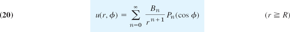
satisfying (8), (9), (10), with coefficients
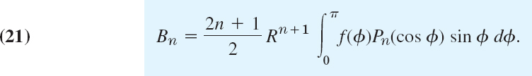
The next example illustrates all this for a sphere of radius 1 consisting of two hemispheres that are separated by a small strip of insulating material along the equator, so that these hemispheres can be kept at different potentials (110 V and 0 V).
Find the potential inside and outside a spherical capacitor consisting of two metallic hemispheres of radius 1 ft separated by a small slit for reasons of insulation, if the upper hemisphere is kept at 110 V and the lower is grounded (Fig. 313).
Solution. The given boundary condition is (recall Fig. 312)

Since R = 1, we thus obtain from (19)

where w = cosφ. Hence Pn(cos φ)sin φ dφ = −Pn(w) we integrate from 1 to 0, and we finally get rid of the minus by integrating from 0 to 1. You can evaluate this integral by your CAS or continue by using (11) in Sec. 5.2, obtaining
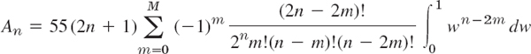
where M = n/2 for even n and M = (n − 1)/2 for odd n. The integral equals 1/(n − 2m + 1). Thus

Fig. 313. Spherical capacitor in Example 1

Taking n = 0, we get A0 = 55 (since 0! = 1). For n = 1, 2, 3, … we get

Hence the potential (17) inside the sphere is (since P0 = 1)
![]()
with P1, P3, … given by (11′), Sec. 5.21. Since R = 1, we see from (19) and (21) in this section that Bn = An and (20) thus gives the potential outside the sphere

Partial sums of these series can now be used for computing approximate values of the inner and outer potential. Also, it is interesting to see that far away from the sphere the potential is approximately that of a point charge, namely, 55/r. (Compare with Theorem 3 in Sec. 9.7.)

Fig. 314. Partial sums of the first 4, 6, and 11 nonzero terms of (23) for r = R = 1
EXAMPLE 2 Simpler Cases. Help with Problems
The technicalities encountered in cases that are similar to the one shown in Example 1 can often be avoided. For instance, find the potential inside the sphere S: r = R = 1 when S is kept at the potential f(φ) = cos 2φ. (Can you see the potential on S? What is it at the North Pole? The equator? The South Pole?)
Solution. ![]() . Hence the potential in the interior of the sphere is
. Hence the potential in the interior of the sphere is
![]()
- Spherical coordinates. Derive (7) from
 in spherical coordinates.
 - Cylindrical coordinates. Verify (5) by transforming
 back into Cartesian coordinates.
 - Sketch Pn(cos θ), 0 θ 2π, for n = 0, 1, 2. (Use (11′) in Sec. 5.2.)
- Zero surfaces. Find the surfaces on which u1, u2, u3 in (16) are zero.
- CAS PROBLEM. Partial Sums. In Example 1 in the text verify the values of A1, A2, A3 and compute A4, … A10. Try to find out graphically how well the corresponding partial sums of (23) approximate the given boundary function.
- CAS EXPERIMENT. Gibbs Phenomenon. Study the Gibbs phenomenon in Example 1 (Fig. 314) graphically.
- Verify that un and
 in (16) are solutions of (8).
8.15 POTENTIALS DEPENDING ONLY ON r
- 8. Dimension 3. Verify that the potential u = c/r, r =
 satisfies Laplace's equation in spherical coordinates.
 - 9. Spherical symmetry. Show that the only solution of Laplace's equation depending only on r =
 is u = c/r + k with constant c and k.
 - 10. Cylindrical symmetry. Show that the only solution of Laplace's equation depending only on
 is u = c ln r + k.
 - 11. Verification. Substituting u(r) with r as in Prob. 9 into uxx + uyy + uzz = 0, verify that u″ + 2u′/r = 0, in agreement with (7).
- 12. Dirichlet problem. Find the electrostatic potential between coaxial cylinders of radii r1 = 2 cm and r2 = 4 cm kept at the potentials U1 = 220 V and U2 = 140 V, respectively.
- 13. Dirichlet problem. Find the electrostatic potential between two concentric spheres of radii r1 = 2 cm and r2 = 4 cm kept at the potentials U1 = 220 V and U2 = 140 V, respectively. Sketch and compare the equipotential lines in Probs. 12 and 13. Comment.
- 14. Heat problem. If the surface of the ball r2 = x2 + y2 + z2 R2 is kept at temperature zero and the initial temperature in the ball is f(r), show that the temperature u(r, t) in the ball is a solution of ut = c2(urr + 2ur/r) satisfying the conditions u(R, t) = 0, u(r, 0) = f(r). Show that setting v = ru gives vt = c2vrr, v(R, t) = 0, v(r, 0) = rf(r). Include the condition v(0, t) = 0 (which holds because u must be bounded at r = 0), and solve the resulting problem by separating variables.
- 15. What are the analogs of Probs. 12 and 13 in heat conduction?
16.20 BOUNDARY VALUE PROBLEMS IN SPHERICAL COORDINATES r, θ, φ,
Find the potential in the interior of the sphere r = R = 1 if the interior is free of charges and the potential on the sphere is
- 16. f(φ) = cos φ
- 17. f(φ) = 1
- 18. f(φ) = 1 − cos2
- 19. f(φ) = cos 2φ
- 20. f(φ) = 10 cos3 φ − 3 cos2 φ − 5 cos φ − 1
- 21. Point charge. Show that in Prob. 17 the potential exterior to the sphere is the same as that of a point charge at the origin.
- 22. Exterior potential. Find the potentials exterior to the sphere in Probs. 16 and 19.
- 23. Plane intersections. Sketch the intersections of the equipotential surfaces in Prob. 16 with xz-plane.
- 24. TEAM PROJECT. Transmission Line and Related PDEs. Consider a long cable or telephone wire (Fig. 315) that is imperfectly insulated, so that leaks occur along the entire length of the cable. The source S of the current i(x, t) in the cable is at x = 0, the receiving end T at x = l. The current flows from S to T and through the load, and returns to the ground. Let the constants R, L, C, and G denote the resistance, inductance, capacitance to ground, and conductance to ground, respectively, of the cable per unit length.

- Show that (“first transmission line equation”)

where u(x, t) is the potential in the cable. Hint: Apply Kirchhoff's voltage law to a small portion of the cable between x and x + Δx (difference of the potentials at x and x + Δx = resistive drop + inductive drop).
- Show that for the cable in (a) (“second transmission line equation”),

Hint: Use Kirchhoff's current law (difference of the currents at x and x + Δx = loss due to leakage to ground + capacitive loss).
- Second-order PDEs. Show that elimination of i or u from the transmission line equations leads to

- Telegraph equations. For a submarine cable, G is negligible and the frequencies are low. Show that this leads to the so-called submarine cable equations or telegraph equations

Find the potential in a submarine cable with ends (x = 0, x = l) grounded and initial voltage distribution U0 = const.
- High-frequency line equations. Show that in the case of alternating currents of high frequencies the equations in (c) can be approximated by the so-called high-frequency line equations

Solve the first of them, assuming that the initial potential is
and ut(x, 0) = 0 and u = 0 at the ends x = 0 and x = l for all t.
- Show that (“first transmission line equation”)
- 25. Reflection in a sphere. Let r, θ, φ be spherical coordinates. If u(r, θ, φ) satisfies
 , show that v(r, θ, φ) = u(1/r, θ, φ)/r satisfies
  .
.
12.12 Solution of PDEs by Laplace Transforms
Readers familiar with Chap. 6 may wonder whether Laplace transforms can also be used for solving partial differential equations. The answer is yes, particularly if one of the independent variables ranges over the positive axis. The steps to obtain a solution are similar to those in Chap. 6. For a PDE in two variables they are as follows.
- Take the Laplace transform with respect to one of the two variables, usually t. This gives an ODE for the transform of the unknown function. This is so since the derivatives of this function with respect to the other variable slip into the transformed equation. The latter also incorporates the given boundary and initial conditions.
- Solving that ODE, obtain the transform of the unknown function.
- Taking the inverse transform, obtain the solution of the given problem.
If the coefficients of the given equation do not depend on t, the use of Laplace transforms will simplify the problem.
We explain the method in terms of a typical example.
EXAMPLE 1 Semi-Infinite String
Find the displacement w(x, t) of an elastic string subject to the following conditions. (We write w since we need u to denote the unit step function.)
- The string is initially at rest on the x-axis from x = 0 to ∞ (“semi-infinite string”).
- For t > 0 the left end of the string (x = 0) is moved in a given fashion, namely, according to a single sine wave

- Furthermore,
 .
.

Fig. 316. Motion of the left end of the string in Example 1 as a function of time t
Of course there is no infinite string, but our model describes a long string or rope (of negligible weight) with its right end fixed far out on the x-axis.
Solution. We have to solve the wave equation (Sec. 12.2)

for positive x and t, subject to the “boundary conditions”
![]()
with f as given above, and the initial conditions
![]()
We take the Laplace transform with respect to t. By (2) in Sec. 6.2,
The expression −sw(x, 0) − wt(x, 0) drops out because of (3). On the right we assume that we may interchange integration and differentiation. Then

Writing W(x, s) = ![]() {w(x, t)}, we thus obtain
{w(x, t)}, we thus obtain
Since this equation contains only a derivative with respect to x, it may be regarded as an ordinary differential equation W(x, s) for considered as a function of x. A general solution is
![]()
From (2) we obtain, writing F(s) = ![]() [f(t)],
[f(t)],
![]()
Assuming that we can interchange integration and taking the limit, we have

This implies A(s) = 0 in (4) because c > 0, so that for every fixed positive s the function esx/e increases as x increases. Note that we may assume s > 0 since a Laplace transform generally exists for all s greater than some fixed k (Sec. 6.2). Hence we have
![]()
so that (4) becomes
![]()
From the second shifting theorem (Sec. 6.3) with we obtain the inverse transform

![]()
and zero otherwise. This is a single sine wave traveling to the right with speed c. Note that a point x remains at rest until t = x/c, the time needed to reach that x if one starts at t = 0 (start of the motion of the left end) and travels with speed c. The result agrees with our physical intuition. Since we proceeded formally, we must verify that (5) satisfies the given conditions. We leave this to the student.

Fig. 317. Traveling wave in Example 1
We have reached the end of Chapter 12, in which we concentrated on the most important partial differential equations (PDEs) in physics and engineering. We have also reached the end of Part C on Fourier Analysis and PDEs.
Outlook
We have seen that PDEs underlie the modeling process of various important engineering application. Indeed, PDEs are the subject of many ongoing research projects.
Numerics for PDEs follows in Secs. 21.4–21.7, which, by design for greater flexibility in teaching, are independent of the other sections in Part E on numerics.
In the next part, that is, Part D on complex analysis, we turn to an area of a different nature that is also highly important to the engineer. The rich vein of examples and problems will signify this. It is of note that Part D includes another approach to the two-dimensional Laplace equation with applications, as shown in Chap. 18.
- Verify the solution in Example 1. What traveling wave do we obtain in Example 1 for a nonterminating sinusoidal motion of the left end starting at t = 2π?
- Sketch a figure similar to Fig. 317 when c = 1 and f(x) is “triangular,” say,
 =
=  and 0 otherwise.
 - How does the speed of the wave in Example 1 of the text depend on the tension and on the mass of the string?
4.8 SOLVE BY LAPLACE TRANSFORMS
- 4.
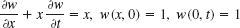
- 5.

- 6.
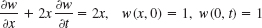
- 7. Solve Prob. 5 by separating variables.
- 8.

Find the temperature w(x, t) in a semi-infinite laterally insulated bar extending from x = 0 along the x-axis to infinity, assuming that the initial temperature is 0, w(x, t)→0 as x→∞ for every fixed t ![]() 0, and w(0, t) = f(t). Proceed as follows.
0, and w(0, t) = f(t). Proceed as follows.
- 9. Set up the model and show that the Laplace transform leads to
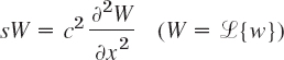
and

- 10. Applying the convolution theorem, show that in Prob. 9,
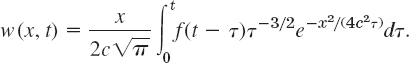
- 11. Let w(0, t) = f(t) = u(t) (Sec. 6.3). Denote the corresponding w, W, and F by w0, W0, and F0. Show that then in Prob. 10,

with the error function erf as defined in Problem Set 12.7.
- 12. Duhamel's formula.4 Show that in Prob. 11,
and the convolution theorem gives Duhamel's formula
CHAPTER 12 REVIEW QUESTIONS AND PROBLEMS
- For what kinds of problems will modeling lead to an ODE? To a PDE?
- Mention some of the basic physical principles or laws that will give a PDE in modeling.
- State three or four of the most important PDEs and their main applications.
- What is “separating variables” in a PDE? When did we apply it twice in succession?
- What is d'Alembert's solution method? To what PDE does it apply?
- What role did Fourier series play in this chapter? Fourier integrals?
- When and why did Legendre's equation occur? Bessel's equation?
- What are the eigenfunctions and their frequencies of the vibrating string? Of the vibrating membrane?
- What do you remember about types of PDEs? Normal forms? Why is this important?
- When did we use polar coordinates? Cylindrical coordinates? Spherical coordinates?
- Explain mathematically (not physically) why we got exponential functions in separating the heat equation, but not for the wave equation.
- Why and where did the error function occur?
- How do problems for the wave equation and the heat equation differ regarding additional conditions?
- Name and explain the three kinds of boundary conditions for Laplace's equation.
- Explain how the Laplace transform applies to PDEs.
16.18 Solve for u = u(x, y):
- 16. uxx + 25u = 0
- 17. uyy + uy − 6u = 18
- 18. uxx + ux = 0, u(0, y) = f(y), ux(0, y) = g(y)
19.21 NORMAL FORM
Transform to normal form and solve:
- 19. uxy = uyy
- 20. uxx + 6uxy + 9uyy = 0
- 21. uxx − 4uyy = 0
22.24 VIBRATING STRING
Find and sketch or graph (as in Fig. 288 in Sec. 12.3) the deflection u(x, t) of a vibrating string of length π, extending from to x = 0 to x = π, and c2 = T/ρ = 4 starting with velocity zero and deflection:
- 22. sin 4x
- 23. sin3x
- 24.

Find the temperature distribution in a laterally insulated thin copper bar c2 = K/(σρ = 1.158 cm2/sec) of length 100 cm and constant cross section with endpoints at x = 0 and 100 kept at 0°C and initial temperature:
- 25. sin 0.01 πx
- 26. 50 − |50 − x|
- 27. sin3 0.1πx
28.30 ADIABATIC CONDITIONS
Find the temperature distribution in a laterally insulated bar of length π with c2 = 1 for the adiabatic boundary condition (see Problem Set 12.6) and initial temperature:
- 28. 3x2
- 29. 100 cos 2x
- 30.

31.32 TEMPERATURE IN A PLATE
- 31. Let f(x, y) = u(x, y, 0) be the initial temperature in a thin square plate of side π with edges kept 0°C at and faces perfectly insulated. Separating variables, obtain from
 the solution
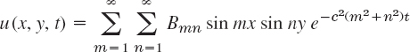
where
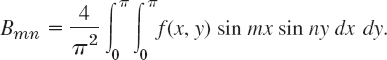
- 32. Find the temperature in Prob. 31 if

33.37 MEMBRANES
Show that the following membranes of area 1 with c2 = 1 have the frequencies of the fundamental mode as given (4-decimal values). Compare.
- 33. Circle:

- 34. Square:

- 35. Rectangle with sides

- 36. Semicircle:

- 37. Quadrant of circle: of circle:
 (α21 = 5.13562 = first positive zero of J2)
38.40 ELECTROSTATIC POTENTIAL
Find the potential in the following charge-free regions.
- 38. Between two concentric spheres of radii r0 and r1 kept at potentials u0 and u1, respectively.
- 39. Between two coaxial circular cylinders of radii r0 and r1 kept at the potentials and u0 and u1, respectively. Compare with Prob. 38.
- 40. In the interior of a sphere of radius 1 kept at the potential f(φ) = cos 3φ + 3 cos φ (referred to our usual spherical coordinates).
SUMMARY OF CHAPTER 12 Partial Differential Equations (PDEs)
Whereas ODEs (Chaps. 1–6) serve as models of problems involving only one independent variable, problems involving two or more independent variables (space variables or time t and one or several space variables) lead to PDEs. This accounts for the enormous importance of PDEs to the engineer and physicist. Most important are:
![]()
![]()
![]()
![]()
![]()
Equations (1) and (2) are hyperbolic, (3) is parabolic, (4) and (5) are elliptic.
In practice, one is interested in obtaining the solution of such an equation in a given region satisfying given additional conditions, such as initial conditions (conditions at time t = 0) or boundary conditions (prescribed values of the solution u or some of its derivatives on the boundary surface S, or boundary curve C, of the region) or both. For (1) and (2) one prescribes two initial conditions (initial displacement and initial velocity). For (3) one prescribes the initial temperature distribution. For (4) and (5) one prescribes a boundary condition and calls the resulting problem a (see Sec. 12.6)
Dirichlet problem if u is prescribed on S,
Neumann problem if un = ∂/∂n is prescribed on S,
Mixed problem if u is prescribed on one part of S and un on the other.
A general method for solving such problems is the method of separating variables or product method, in which one assumes solutions in the form of products of functions each depending on one variable only. Thus equation (1) is solved by setting u(x, t) = F(x)G(t); see Sec. 12.3; similarly for (3) (see Sec. 12.6). Substitution into the given equation yields ordinary differential equations for F and G, and from these one gets infinitely many solutions F = Fn and G = Gn such that the corresponding functions
![]()
are solutions of the PDE satisfying the given boundary conditions. These are the eigenfunctions of the problem, and the corresponding eigenvalues determine the frequency of the vibration (or the rapidity of the decrease of temperature in the case of the heat equation, etc.). To satisfy also the initial condition (or conditions), one must consider infinite series of the un, whose coefficients turn out to be the Fourier coefficients of the functions f and g representing the given initial conditions (Secs. 12.3, 12.6). Hence Fourier series (and Fourier integrals) are of basic importance here (Secs. 12.3, 12.6, 12.7, 12.9).
Steady-state problems are problems in which the solution does not depend on time t. For these, the heat equation ![]() becomes the Laplace equation.
becomes the Laplace equation.
Before solving an initial or boundary value problem, one often transforms the PDE into coordinates in which the boundary of the region considered is given by simple formulas. Thus in polar coordinates given by x = r cos θ, y = r sin θ, the Laplacian becomes (Sec. 12.11)

for spherical coordinates see Sec. 12.10. If one now separates the variables, one gets Bessel's equation from (2) and (6) (vibrating circular membrane, Sec. 12.10) and Legendre's equation from (5) transformed into spherical coordinates (Sec. 12.11).
1 JEAN LE ROND D'ALEMBERT (1717–1783), French mathematician, also known for his important work in mechanics.
We mention that the general theory of PDEs provides a systematic way for finding the transformation (2) that simplifies (1). See Ref. [C8] in App. 1.
2Sir GEORGE BIDELL AIRY (1801–1892), English mathematician, known for his work in elasticity. FRANCESCO TRICOMI (1897–1978), Italian mathematician, who worked in integral equations and functional analysis.
3HERMANN VON HELMHOLTZ (1821–1894), German physicist, known for his fundamental work in thermodynamics, fluid flow, and acoustics.
4JEAN–MARIE CONSTANT DUHAMEL (1797–1872), French mathematician.