
CHAPTER 17
Conformal Mapping

Conformal mappings are invaluable to the engineer and physicist as an aid in solving problems in potential theory. They are a standard method for solving boundary value problems in two-dimensional potential theory and yield rich applications in electrostatics, heat flow, and fluid flow, as we shall see in Chapter 18.
The main feature of conformal mappings is that they are angle-preserving (except at some critical points) and allow a geometric approach to complex analysis. More details are as follows. Consider a complex w = f(z) function defined in a domain D of the z–plane; then to each point in D there corresponds a point in the w-plane. In this way we obtain a mapping of D onto the range of values of f (z) in the w- plane. In Sec. 17.1 we show that if f(z) is an analytic function, then the mapping given by w = f(z) is a conformal mapping, that is, it preserves angles, except at points where the derivative f′(z) is zero. (Such points are called critical points.)
Conformality appeared early in the history of construction of maps of the globe. Such maps can be either “conformal,” that is, give directions correctly, or “equiareal,” that is, give areas correctly except for a scale factor. However, the maps will always be distorted because they cannot have both properties, as can be proven, see [GenRef8] in App. 1. The designer of accurate maps then has to select which distortion to take into account.
Our study of conformality is similar to the approach used in calculus where we study properties of real functions y = f(x) and graph them. Here we study the properties of conformal mappings (Secs. 17.1–17.4) to get a deeper understanding of the properties of functions, most notably the ones discussed in Chap. 13. Chapter 17 ends with an introduction to Riemann surfaces, an ingenious geometric way of dealing with multivalued complex functions such as w = sqrt (z) and w = ln z.
So far we have covered two main approaches to solving problems in complex analysis. The first one was solving complex integrals by Cauchy's integral formula and was broadly covered by material in Chaps. 13 and 14. The second approach was to use Laurent series and solve complex integrals by residue integration in Chaps. 15 and 16. Now, in Chaps. 17 and 18, we develop a third approach, that is, the geometric approach of conformal mapping to solve boundary value problems in complex analysis.
Prerequisite: Chap. 13.
Sections that may be omitted in a shorter course:17.3 and 17.5.
References and Answers to Problems: App. 1 Part D, App. 2.
17.1 Geometry of Analytic Functions: Conformal Mapping
We shall see that conformal mappings are those mappings that preserve angles, except at critical points, and that these mappings are defined by analytic functions. A critical point occurs wherever the derivative of such a function is zero. To arrive at these results, we have to define terms more precisely.
A complex function
![]()
of a complex variable z gives a mapping of its domain of definition D in the complex z-plane into the complex w-plane or onto its range of values in that plane.1 For any point z0 in D the point w0 = f(z0) is called the image of z0 with respect to f. More generally, for the points of a curve C in D the image points form the image of C; similarly for other point sets in D. Also, instead of the mapping by a function w = f(z) we shall say more briefly the mapping. w = f(z).
EXAMPLE 1 Mapping w = f(x) = z2
Using polar forms z = reiθ and w = Reiø, we have w = z2 = r2e2iθ. Comparing moduli and arguments gives R = r2 and ø = 2θ. Hence circles r = r0 are mapped onto circles ![]() and rays θ = θ0 onto rays ø = 2θ0. Figure 378 shows this for the region
and rays θ = θ0 onto rays ø = 2θ0. Figure 378 shows this for the region ![]() π/6
π/6 ![]() θ
θ ![]() π/3, which is mapped onto the region
π/3, which is mapped onto the region ![]() , π/3
, π/3 ![]() θ
θ ![]() 2π/3.
2π/3.
In Cartesian coordinates we have z = x + iy and
![]()
Hence vertical lines x = c = const are mapped onto u = c2 − y2, v = 2cy. From this we can eliminate y. We obtain y2 = c2 − u and v2 = 4c2y2. Together,
![]()
These parabolas open to the left. Similarly, horizontal lines y = k = const are mapped onto parabolas opening to the right,
![]()

Fig. 378. Mapping w = z2. Lines |z| = const, arg z = const and their images in the w-plane

Fig. 379. Images of x = const, y = const under w = z2
Conformal Mapping
A mapping w = f(z) is called conformal if it preserves angles between oriented curves in magnitude as well as in sense. Figure 380 shows what this means. The angle α (0 ![]() α
α ![]() π) between two intersecting curves C1 and C2 is defined to be the angle between their oriented tangents at the intersection point z0. And conformality means that the images
π) between two intersecting curves C1 and C2 is defined to be the angle between their oriented tangents at the intersection point z0. And conformality means that the images ![]() and
and ![]() of C1 and C2 make the same angle as the curves themselves in both magnitude and direction.
of C1 and C2 make the same angle as the curves themselves in both magnitude and direction.
THEOREM 1 Conformality of Mapping by Analytic Functions
The mapping w = f(z) by an analytic function f is conformal, except at critical points, that is, points at which the derivative f′ is zero.
PROOF
w = z2 has a critical point at z = 0, where f′(z) = 2z = 0 and the angles are doubled (see Fig. 378), so that conformality fails.
The idea of proof is to consider a curve
![]()
in the domain of f(z) and to show that w = f(z) rotates all tangents at a point z0 (where f′(z0) ≠ 0) through the same angle. Now ![]() is tangent to C in (2) because this is the limit of (z1 − z0)/Δt (which has the direction of the secant z1 −z0 in Fig. 381) as z1 approaches z0 along C. The image C* of C is w = f(z(t)). By the chain rule,
is tangent to C in (2) because this is the limit of (z1 − z0)/Δt (which has the direction of the secant z1 −z0 in Fig. 381) as z1 approaches z0 along C. The image C* of C is w = f(z(t)). By the chain rule, ![]() Hence the tangent direction of C* is given by the argument (use (9) in Sec. 13.2)
Hence the tangent direction of C* is given by the argument (use (9) in Sec. 13.2)
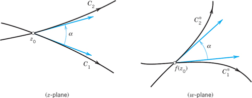
Fig. 380. Curves C1 and C2 and their respective images ![]() and
and ![]() under a conformal mapping w = f(z)
under a conformal mapping w = f(z)
where arg ![]() gives the tangent direction of C. This shows that the mapping rotates all directions at a point z0 in the domain of analyticity of f through the same angle arg f′(z0), which exists as long as f′(z0) ≠ 0. But this means conformality, as Fig. 381 illustrates for an angle α between two curves, whose images
gives the tangent direction of C. This shows that the mapping rotates all directions at a point z0 in the domain of analyticity of f through the same angle arg f′(z0), which exists as long as f′(z0) ≠ 0. But this means conformality, as Fig. 381 illustrates for an angle α between two curves, whose images ![]() and
and ![]() make the same angle (because of the rotation).
make the same angle (because of the rotation).

Fig. 381. Secant and tangent of the curve C
In the remainder of this section and in the next ones we shall consider various conformal mappings that are of practical interest, for instance, in modeling potential problems.
EXAMPLE 2 Conformality of w = zn
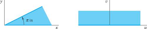
The mapping w = zn, n = 2, 3, …, is conformal, except at z = 0, where w′ = nzn−1 = 0. For n = 0 this is shown in Fig. 378; we see that at 0 the angles are doubled. For general n the angles at 0 are multiplied by a factor n under the mapping. Hence the sector 0 ![]() θ
θ ![]() π/n is mapped by zn onto the upper half-plane v
π/n is mapped by zn onto the upper half-plane v ![]() 0 (Fig. 382).
0 (Fig. 382).
EXAMPLE 3 Mapping w = z + 1/z. Joukowski Airfoil
In terms of polar coordinates this mapping is
![]()
By separating the real and imaginary parts we thus obtain
![]()
Hence circles |z| = r = const ≠ 1 are mapped onto ellipses x2/a2 + y2/b2 = 1. The circle r = 1 is mapped onto the segment −2 ![]() u
u ![]() 2 of the u-axis. See Fig. 383.
2 of the u-axis. See Fig. 383.
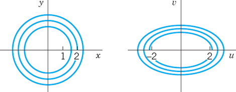
Fig. 383. Example 3
Now the derivative of w is
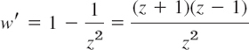
which is 0 at z = ±1. These are the points at which the mapping is not conformal. The two circles in Fig. 384 pass through z = −1. The larger is mapped onto a Joukowski airfoil. The dashed circle passes through both −1 and 1 and is mapped onto a curved segment.
Another interesting application of w = z + 1/z (the flow around a cylinder) will be considered in Sec. 18.4.

EXAMPLE 4 Conformality of w = ez
From (10) in Sec. 13.5 we have |ez| = ex and Arg z = y. Hence ez maps a vertical straight line x = x0 = const onto the circle |w| = ex0 and a horizontal straight line y = y0 = const onto the ray arg w = y0. The rectangle in Fig. 385 is mapped onto a region bounded by circles and rays as shown.
The fundamental region −π < Arg z ![]() π of ez in the z-plane is mapped bijectively and conformally onto the entire w-plane without the origin w = 0 (because ez = 0 for no z). Figure 386 shows that the upper half 0 < y
π of ez in the z-plane is mapped bijectively and conformally onto the entire w-plane without the origin w = 0 (because ez = 0 for no z). Figure 386 shows that the upper half 0 < y ![]() π of the fundamental region is mapped onto the upper half-plane 0 < arg w
π of the fundamental region is mapped onto the upper half-plane 0 < arg w ![]() π, the left half being mapped inside the unit disk |w|
π, the left half being mapped inside the unit disk |w| ![]() 1 and the right half outside (why?).
1 and the right half outside (why?).

EXAMPLE 5 Principle of Inverse Mapping. Mapping w = Ln z
Principle. The mapping by the inverse z = f−1(w) of w = f(z) is obtained by interchanging the roles of the z-plane and the w-plane in the mapping by w = f(z).
Now the principal value w = f(z) = Ln z of the natural logarithm has the inverse z = f−1(w) = ew. From Example 4 (with the notations z and w interchanged!) we know that f−1(w) = ew maps the fundamental region of the exponential function onto the z-plane without z = 0 (because ew ≠ 0 for every w). Hence w = f(z) = Ln z maps the z-plane without the origin and cut along the negative real axis (where θ = Im Ln z jumps by 2π) conformally onto the horizontal strip −π < v ![]() π of the w-plane, where w = u + iv.
π of the w-plane, where w = u + iv.
Since the mapping w = Ln z + 2πi differs from w = Ln z by the translation 2πi (vertically upward), this function maps the z-plane (cut as before and 0 omitted) onto the strip π < v ![]() 3π. Similarly for each of the infinitely many mappings w = ln z = Ln z ± 2nπi (n = 0, 1, 2, …). The corresponding horizontal strips of width 2π (images of the z-plane under these mappings) together cover the whole w-plane without overlapping.
3π. Similarly for each of the infinitely many mappings w = ln z = Ln z ± 2nπi (n = 0, 1, 2, …). The corresponding horizontal strips of width 2π (images of the z-plane under these mappings) together cover the whole w-plane without overlapping.
Magnification Ratio. By the definition of the derivative we have
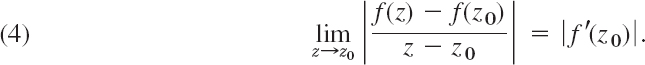
Therefore, the mapping w = f(z) magnifies (or shortens) the lengths of short lines by approximately the factor |f′(z0)|. The image of a small figure conforms to the original figure in the sense that it has approximately the same shape. However, since f′(z) varies from point to point, a large figure may have an image whose shape is quite different from that of the original figure.
More on the Condition f′(z) ≠ 0. From (4) in Sec. 13.4 and the Cauchy–Riemann equations we obtain

that is,
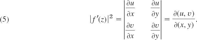
This determinant is the so-called Jacobian (Sec. 10.3) of the transformation w = f(z) written in real form u = u(x, y), v = v(x, y). Hence f′(z0) ≠ 0 implies that the Jacobian is not 0 at z0. This condition is sufficient that the mapping w = f(z) in a sufficiently small neighborhood of z0 is one-to-one or injective (different points have different images). See Ref. [GenRef4] in App. 1.
- On Fig. 378. One “rectangle” and its image are colored. Identify the images for the other “rectangles.”
- On Example 1. Verify all calculations.
- Mapping w = z3. Draw an analog of Fig. 378 for w = z3.
- Conformality. Why do the images of the straight lines x = const and y = const under a mapping by an analytic function intersect at right angles? Same question for the curves |z| = const and arg z = const. Are there exceptional points?
- Experiment on w =
 . Find out whether w = preserves angles in size as well as in sense. Try to prove your result.
6–9 MAPPING OF CURVES
Find and sketch or graph the images of the given curves under the given mapping.
- 6. x = 1, 2, 3, 4, y = 1, 2, 3, 4, w = z2
- 7. Rotation. Curves as in Prob. 6, w = iz
- 8. Reflection in the unit circle.
 Arg z = 0, ±π/4, ±π/2, ±3π/2
 - 9. Translation. Curves as in Prob. 6, w = z + 2 + i
- 10. CAS EXPERIMENT. Orthogonal Nets. Graph the orthogonal net of the two families of level curves Re f(z) = const and Im f(z) = const, where (a) f(z) = z4, (b) f(z) = 1/z, (c) f(z) = 1/z2, (d) f(z) = (z + i)/(1 + iz). Why do these curves generally intersect at right angles? In your work, experiment to get the best possible graphs. Also do the same for other functions of your own choice. Observe and record shortcomings of your CAS and means to overcome such deficiencies.
11–20 MAPPING OF REGIONS
Sketch or graph the given region and its image under the given mapping.
- 11.
 −π/8 < Arg z < π/8, w = z2
 - 12. 1 < |z| < 3, 0 < Arg z < π/2, w = z3
- 13. 2
 Im z 5, w = iz
 - 14. x
 1, w = 1/z
 - 15.
 w = 1/z
 - 16.
 Im z > 0, w = 1/z
 - 17. − Ln 2 x 4, w = ez
- 18. −1 x 2, −π < y < π, w = ez
- 19. 1 < |z| < 4, π/4 < θ 3π/4, w = Ln z
- 20.
 0 θ < π/2, w = Ln z
21–26 FAILURE OF CONFORMALITY
Find all points at which the mapping is not conformal. Give reason.
- 21. A cubic polynomial
- 22. z2 + 1/z2
- 23.

- 24. exp (z5 − 80z)
- 25. cosh z
- 26. sin π z
- 27. Magnification of Angles. Let f(z) be analytic at z0. Suppose that f′(z0) = 0, …, f(k−1)(z0) = 0. Then the mapping w = f(z) magnifies angles with vertex at z0 by a factor k. Illustrate this with examples for k = 2, 3, 4.
- 28. Prove the statement in Prob. 27 for general k = 1, 2, …. Hint. Use the Taylor series.
29–35 MAGNIFICATION RATIO, JACOBIAN
Find the magnification ratio M. Describe what it tells you about the mapping. Where is M = 1? Find the Jacobian J.
- 29.

- 30. w = z3
- 31. w = 1/z
- 32. w = 1/z2
- 33. w = ez
- 34.

- 35. w = Ln z
17.2 Linear Fractional Transformations (Möbius Transformations)
Conformal mappings can help in modeling and solving boundary value problems by first mapping regions conformally onto another. We shall explain this for standard regions (disks, half-planes, strips) in the next section. For this it is useful to know properties of special basic mappings. Accordingly, let us begin with the following very important class.
The next two sections discuss linear fractional transformations. The reason for our thorough study is that such transformations are useful in modeling and solving boundary value problems, as we shall see in Chapter 18. The task is to get a good grasp of which conformal mappings map certain regions conformally onto each other, such as, say mapping a disk onto a half-plane (Sec. 17.3) and so forth. Indeed, the first step in the modeling process of solving boundary value problems is to identify the correct conformal mapping that is related to the “geometry” of the boundary value problem.
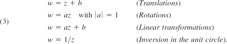
The following class of conformal mappings is very important. Linear fractional transformations (or Möbius transformations) are mappings

where a, b, c, d are complex or real numbers. Differentiation gives

This motivates our requirement ad − bc ≠ 0. It implies conformality for all z and excludes the totally uninteresting case w′ ≡ 0 once and for all. Special cases of (1) are
EXAMPLE 1 Properties of the Inversion w = 1/z(Fig. 387)
In polar forms z = reiθ and w = Reiø the inversion w = 1/z is
![]()
Hence the unit circle |z| = r = 1 is mapped onto the unit circle |w| = R = 1; w = eiø = e−iθ. For a general z the image w = 1/z can be found geometrically by marking |w| = R = 1/r on the segment from 0 to z and then reflecting the mark in the real axis. (Make a sketch.)
Figure 387 shows that w = 1/z maps horizontal and vertical straight lines onto circles or straight lines. Even the following is true.
![]()

Fig. 387. Mapping (Inversion) w = 1/z
Proof. Every straight line or circle in the z-plane can be written
![]()
A = 0 gives a straight line and A ≠ 0 a circle. In terms of z and ![]() this equation becomes
this equation becomes
![]()
Now w = 1/z. Substitution of z = 1/w and multiplication by ![]() gives the equation
gives the equation
![]()
or, in terms of u and v,
![]()
This represents a circle (if D ≠ 0 or a straight line (if D = 0 in the w-plane.
The proof in this example suggests the use of z and ![]() instead of x and y, a general principle that is often quite useful in practice.
instead of x and y, a general principle that is often quite useful in practice.
Surprisingly, every linear fractional transformation has the property just proved:
THEOREM 1 Circles and Straight Lines
Every linear fractional transformation (1) maps the totality of circles and straight lines in the z-plane onto the totality of circles and straight lines in the w-plane.
PROOF
This is trivial for a translation or rotation, fairly obvious for a uniform expansion or contraction, and true for w = 1/z, as just proved. Hence it also holds for composites of these special mappings. Now comes the key idea of the proof: represent (1) in terms of these special mappings. When c = 0, this is easy. When c ≠ 0, the representation is
![]()
This can be verified by substituting K, taking the common denominator and simplifying; this yields (1). We can now set
![]()
and see from the previous formula that then w = w4 + a/c. This tells us that (1) is indeed a composite of those special mappings and completes the proof.
Extended Complex Plane
The extended complex plane (the complex plane together with the point ∞ in Sec. 16.2) can now be motivated even more naturally by linear fractional transformations as follows.
To each z for which cz + d ≠ 0 there corresponds a unique w in (1). Now let c ≠ 0. Then for z = −d/c we have cz + d = 0, so that no w corresponds to this z. This suggests that we let w = ∞ be the image of z = −d/c.
Also, the inverse mapping of (1) is obtained by solving (1) for z; this gives again a linear fractional transformation

When c ≠ 0, then cw − a = 0 for w = a/c, and we let a/c be the image of z = ∞. With these settings, the linear fractional transformation (1) is now a one-to-one mapping of the extended z-plane onto the extended w-plane. We also say that every linear fractional transformation maps “the extended complex plane in a one-to-one manner onto itself.”
Our discussion suggests the following.
General Remark. If z = ∞, then the right side of (1) becomes the meaningless expression (a · ∞ + b)/(c · ∞ + d). We assign to it the value w = a/c if c ≠ 0 and w = ∞ if c = 0.
Fixed Points
Fixed points of a mapping w = f(z) are points that are mapped onto themselves, are “kept fixed” under the mapping. Thus they are obtained from
![]()
The identity mapping w = z has every point as a fixed point. The mapping w = ![]() has infinitely many fixed points, w = 1/z has two, a rotation has one, and a translation none in the finite plane. (Find them in each case.) For (1), the fixed-point condition w = z is
has infinitely many fixed points, w = 1/z has two, a rotation has one, and a translation none in the finite plane. (Find them in each case.) For (1), the fixed-point condition w = z is

For c ≠ 0 this is a quadratic equation in z whose coefficients all vanish if and only if the mapping is the identity mapping w = z (in this case, a = d ≠ 0, b = c = 0). Hence we have
A linear fractional transformation, not the identity, has at most two fixed points. If a linear fractional transformation is known to have three or more fixed points, it must be the identity mapping w = z.
To make our present general discussion of linear fractional transformations even more useful from a practical point of view, we extend it by further facts and typical examples, in the problem set as well as in the next section.
- Verify the calculations in the proof of Theorem 1, including those for the case c = 0.
- Composition of LFTs. Show that substituting a linear fractional transformation (LFT) into an LFT gives an LFT.
- Matrices. If you are familiar with 2 × 2 matrices, prove that the coefficient matrices of (1) and (4) are inverses of each other, provided that ad − bc = 1, and that the composition of LFTs corresponds to the multiplication of the coefficient matrices.
- Fig. 387. Find the image of x = k = const under w = 1/z. Hint. Use formulas similar to those in Example 1.
- Inverse. Derive (4) from (1) and conversely.
- Fixed points. Find the fixed points mentioned in the text before formula (5).
7–10 INVERSE
Find the inverse z = z(w). Check by solving z(w) for w.
- 7.

- 8.

- 9.

- 10.

11–16 FIXED POINTS
Find the fixed points.
- 11. w = (a + ib)z2
- 12. w = z − 3i
- 13. w = 16z5
- 14. w = az + b
- 15.

- 16.
 a ≠ 1
a ≠ 1
17–20 FIXED POINTS
Find all LFTs with fixed point (s).
- 17. z = 0
- 18. z = ±1
- 19. z = ±i
- 20. Without any fixed points
17.3 Special Linear Fractional Transformations
We continue our study of linear fractional transformations. We shall identify linear fractional transformations

that map certain standard domains onto others. Theorem 1 (below) will give us a tool for constructing desired linear fractional transformations.
A mapping (1) is determined by a, b, c, d, actually by the ratios of three of these constants to the fourth because we can drop or introduce a common factor. This makes it plausible that three conditions determine a unique mapping (1):
THEOREM 1 Three Points and Their Images Given
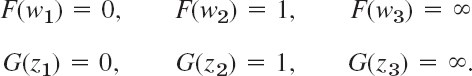
Three given distinct points z1, z2, z3 can always be mapped onto three prescribed distinct points w1, w2, w3 by one, and only one, linear fractional transformation w = f(z). This mapping is given implicitly by the equation

(If one of these points is the point ∞, the quotient of the two differences containing this point must be replaced by 1.)
PROOF
Equation (2) is of the form F(w) = G(z) with linear fractional F and G. Hence w = F−1(G(z)) = f(z), where F−1 is the inverse of F and is linear fractional (see (4) in Sec. 17.2) and so is the composite F−1(G(z)) (by Prob. 2 in Sec. 17.2), that is, w = f(z) is linear fractional. Now if in (2) we set w = w1, w2, w3 on the left and z = z1, z2, z3 on the right, we see that
From the first column, F(w1) = G(z1), thus w1 = F−1(G(z1)) = f(z1). Similarly, w2 = f(z2), w2 = f(z3). This proves the existence of the desired linear fractional transformation.
To prove uniqueness, let w = g(z) be a linear fractional transformation, which also maps zj onto wj, j = 1, 2, 3. Thus wj = g(zj). Hence g−1(wj) = zj, where wj = f(zj). Together, g−1(f(zj)) = zj, a mapping with the three fixed points z1, z2, z3. By Theorem 2 in Sec. 17.2, this is the identity mapping, g−1(f(z)) = z for all z. Thus f(z) = g(z) for all z, the uniqueness.
The last statement of Theorem 1 follows from the General Remark in Sec. 17.2.
Mapping of Standard Domains by Theorem 1
Using Theorem 1, we can now find linear fractional transformations of some practically useful domains (here called “standard domains”) according to the following principle.
Principle. Prescribe three boundary points z1, z2, z3 of the domain D in the z-plane. Choose their images w1, w2, w3 on the boundary of the image D* of D in the w-plane. Obtain the mapping from (2). Make sure that D is mapped onto not D*, onto its complement. In the latter case, interchange two w-points. (Why does this help?)

Fig. 388. Linear fractional transformation in Example 1
EXAMPLE 1 Mapping of a Half-Plane onto a Disk (Fig. 388)
Find the linear fractional transformation (1) that maps z1 = −1, z2 = 0, z3 = 1 onto w1 = −1, w2 = −i w3 = 1, respectively.
Solution. From (2) we obtain

Let us show that we can determine the specific properties of such a mapping without much calculation. For z = x we have w = (x − i)/(−ix + 1), thus |w| = 1, so that the x-axis maps onto the unit circle. Since z = i gives w = 0, the upper half-plane maps onto the interior of that circle and the lower half-plane onto the exterior. z = 0, i, ∞ go onto w = −i, 0, i, so that the positive imaginary axis maps onto the segment S: u = 0, −1 ![]() v
v ![]() 1. The vertical lines x = const map onto circles (by Theorem 1, Sec. 17.2) through w = i (the image of z = ∞) and perpendicular to |w| = 1 (by conformality; see Fig. 388). Similarly, the horizontal lines y = const map onto circles through w = i and perpendicular to S (by conformality). Figure 388 gives these circles for y
1. The vertical lines x = const map onto circles (by Theorem 1, Sec. 17.2) through w = i (the image of z = ∞) and perpendicular to |w| = 1 (by conformality; see Fig. 388). Similarly, the horizontal lines y = const map onto circles through w = i and perpendicular to S (by conformality). Figure 388 gives these circles for y ![]() 0, and for y < 0 they lie outside the unit disk shown.
0, and for y < 0 they lie outside the unit disk shown.
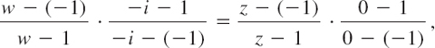
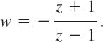
Determine the linear fractional transformation that maps z1 = 0, z2 = 1, z3 = ∞ onto w1 = −1, w2 = −i, w3 = 1, respectively.
Solution. From (2) we obtain the desired mapping

This is sometimes called the Cayley transformation.2 In this case, (2) gave at first the quotient (1 − ∞)/(z − ∞), which we had to replace by 1.
EXAMPLE 3 Mapping of a Disk onto a Half-Plane
Find the linear fractional transformation that maps z1 = −1, z2 = i, z3 = 1 onto w1 = 0, w2 = i, w3 = ∞, respectively, such that the unit disk is mapped onto the right half-plane. (Sketch disk and half-plane.)
Solution. From (2) we obtain, after replacing (i − ∞)/(w − ∞) by 1,
Mapping half-planes onto half-planes is another task of practical interest. For instance, we may wish to map the upper half-plane y ![]() 0 onto the upper half-plane v
0 onto the upper half-plane v ![]() 0. Then the x-axis must be mapped onto the u-axis.
0. Then the x-axis must be mapped onto the u-axis.
EXAMPLE 4 Mapping of a Half-Plane onto a Half-Plane
Find the linear fractional transformation that maps z1 = −2, z2 = 0, z3 = 2 onto w1 = ∞, ![]() respectively.
respectively.
Solution. You may verify that (2) gives the mapping function
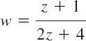
What is the image of the x-axis? Of the y-axis?
Mappings of disks onto disks is a third class of practical problems. We may readily verify that the unit disk in the z-plane is mapped onto the unit disk in the w-plane by the following function, which maps z0 onto the center w = 0.
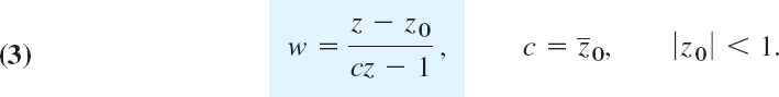
To see this, take |z| = 1, obtaining, with c = ![]() 0 as in (3),
0 as in (3),

Hence
![]()
from (3), so that |z| = 1 maps onto |w| = 1, as claimed, with z0 going onto 0, as the numerator in (3) shows.
Formula (3) is illustrated by the following example. Another interesting case will be given in Prob. 17 of Sec. 18.2.
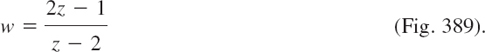

Fig. 389. Mapping in Example 5
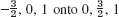
EXAMPLE 6 Mapping of an Angular Region onto the Unit Disk
Certain mapping problems can be solved by combining linear fractional transformations with others. For instance, to map the angular region D: −π/6 ![]() arg z
arg z ![]() π/6 (Fig. 390) onto the unit disk |w|
π/6 (Fig. 390) onto the unit disk |w| ![]() 1, we may map D by Z = z3 onto the right Z-half-plane and then the latter onto the disk |w|
1, we may map D by Z = z3 onto the right Z-half-plane and then the latter onto the disk |w| ![]() 1 by
1 by

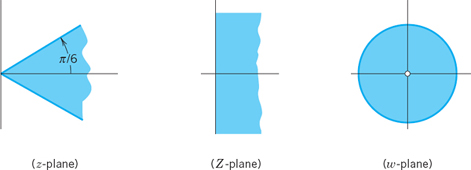
Fig. 390. Mapping in Example 6
This is the end of our discussion of linear fractional transformations. In the next section we turn to conformal mappings by other analytic functions (sine, cosine, etc.).
- CAS EXPERIMENT. Linear Fractional Transformations (LFTs). (a) Graph typical regions (squares, disks, etc.) and their images under the LFTs in Examples 1–5 of the text.
- (b) Make an experimental study of the continuous dependence of LFTs on their coefficients. For instance, change the LFT in Example 4 continuously and graph the changing image of a fixed region (applying animation if available).
- Inverse. Find the inverse of the mapping in Example 1. Show that under that inverse the lines x = const are the images of circles in the w-plane with centers on the line v = 1.
- Inverse. If w = f(z) is any transformation that has an inverse, prove the (trivial!) fact that f and its inverse have the same fixed points.
- Obtain the mapping in Example 1 of this section from Prob. 18 in Problem Set 17.2.
- Derive the mapping in Example 2 from (2).
- Derive the mapping in Example 4 from (2). Find its inverse and the fixed points.
- Verify the formula for disks.
8–16 LFTs FROM THREE POINTS AND IMAGES
Find the LFT that maps the given three points onto the three given points in the respective order.
- 8. 0, 1, 2 onto

- 9. 1, i, −1 onto i, −1, −i
- 10. 0, −i, i onto −1, 0, ∞
- 11. −1, 0, 1 onto −i, −1, i
- 12. 0, 2i, −2i onto −1, 0, ∞
- 13. 0, 1, ∞ onto ∞, 1, 0
- 14. −1, 0, 1 onto 1, 1 + i, 1 + 2i
- 15. 1, i, 2 onto 0, −i, − 1, −

- 16.
- 17. Find an LFT that maps |z| 1 onto |w| 1 so that z = i/2 is mapped onto w = 0. Sketch the images of the lines x = const and y = const.
- 18. Find all LFTs w(z) that map the x-axis onto the u-axis.
- 19. Find an analytic function w = f(z) that maps the region 0 arg z π/4 onto the unit disk |w| 1.
- 20. Find an analytic function that maps the second quadrant of the z-plane onto the interior of the unit circle in the w-plane.
17.4 Conformal Mapping by Other Functions
We shall now cover mappings by trigonometric and hyperbolic analytic functions. So far we have covered the mappings by zn and ez (Sec. 17.1) as well as linear fractional transformations (Secs. 17.2 and 17.3).
Sine Function. Figure 391 shows the mapping by
![]()
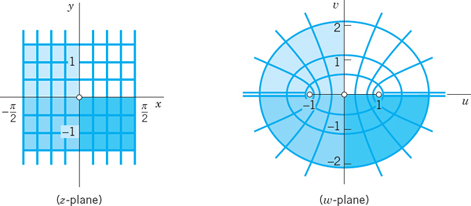
Fig. 391. Mapping w = u + iv = sin z
Hence
![]()
Since sin z is periodic with period 2π, the mapping is certainly not one-to-one if we consider it in the full z-plane. We restrict z to the vertical strip ![]() in Fig. 391. Since f′(z) = cos z = 0 at
in Fig. 391. Since f′(z) = cos z = 0 at ![]() the mapping is not conformal at these two critical points. We claim that the rectangular net of straight lines x = const and y = const in Fig. 391 is mapped onto a net in the w-plane consisting of hyperbolas (the images of the vertical lines x = const) and ellipses (the images of the horizontal lines y = const) intersecting the hyperbolas at right angles (conformality!). Corresponding calculations are simple. From (2) and the relations sin2 x + cos2 x = 1 and cosh2 y − sinh2 y = 1 we obtain
the mapping is not conformal at these two critical points. We claim that the rectangular net of straight lines x = const and y = const in Fig. 391 is mapped onto a net in the w-plane consisting of hyperbolas (the images of the vertical lines x = const) and ellipses (the images of the horizontal lines y = const) intersecting the hyperbolas at right angles (conformality!). Corresponding calculations are simple. From (2) and the relations sin2 x + cos2 x = 1 and cosh2 y − sinh2 y = 1 we obtain
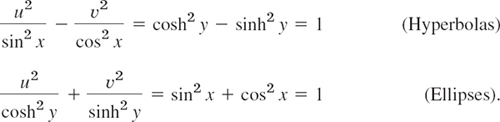
Exceptions are the vertical lines ![]() which are “folded” onto u
which are “folded” onto u ![]() −1 and u
−1 and u ![]() 1 (v = 0), respectively.
1 (v = 0), respectively.
Figure 392 illustrates this further. The upper and lower sides of the rectangle are mapped onto semi-ellipses and the vertical sides onto −cosh 1 ![]() u
u ![]() −1 and 1
−1 and 1 ![]() u
u ![]() cosh 1 (v = 0), respectively. An application to a potential problem will be given in Prob. 3 of Sec. 18.2.
cosh 1 (v = 0), respectively. An application to a potential problem will be given in Prob. 3 of Sec. 18.2.
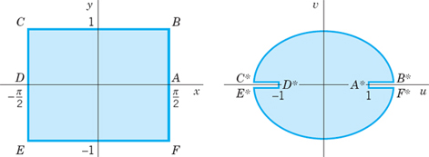
Fig. 392. Mapping by w = sin z
Cosine Function. The mapping w = cos z could be discussed independently, but since
![]()
we see at once that this is the same mapping as sin z preceded by a translation to the right through ![]() π units.
π units.
Hyperbolic Sine. Since
![]()
the mapping is a counterclockwise rotation Z = iz through ![]() π (i.e., 90°), followed by the sine mapping Z* = sin Z, followed by a clockwise 90°-rotation w = −iZ*.
π (i.e., 90°), followed by the sine mapping Z* = sin Z, followed by a clockwise 90°-rotation w = −iZ*.
Hyperbolic Cosine. This function
![]()
defines a mapping that is a rotation Z = iz followed by the mapping w = cos Z.
Figure 393 shows the mapping of a semi-infinite strip onto a half-plane by w = cosh z. Since cosh 0 = 1, the point z = 0 is mapped onto w = 1. For real z = x ![]() 0, cosh z is real and increases with increasing x in a monotone fashion, starting from 1. Hence the positive x-axis is mapped onto the portion u
0, cosh z is real and increases with increasing x in a monotone fashion, starting from 1. Hence the positive x-axis is mapped onto the portion u ![]() 1 of the u-axis.
1 of the u-axis.
For pure imaginary z = iy we have cosh iy = cos y. Hence the left boundary of the strip is mapped onto the segment 1 ![]() u
u ![]() −1 of the u-axis, the point z = πi corresponding to
−1 of the u-axis, the point z = πi corresponding to
![]()
On the upper boundary of the strip, y = π, and since sin π = 0 and cos π = −1, it follows that this part of the boundary is mapped onto the portion u ![]() −1 of the u-axis. Hence the boundary of the strip is mapped onto the u-axis. It is not difficult to see that the interior of the strip is mapped onto the upper half of the w-plane, and the mapping is one-to-one.
−1 of the u-axis. Hence the boundary of the strip is mapped onto the u-axis. It is not difficult to see that the interior of the strip is mapped onto the upper half of the w-plane, and the mapping is one-to-one.
This mapping in Fig. 393 has applications in potential theory, as we shall see in Prob. 12 of Sec. 18.3.
Fig. 393. Mapping by w = cosh z
Tangent Function. Figure 394 shows the mapping of a vertical infinite strip onto the unit circle by w = tan z, accomplished in three steps as suggested by the representation (Sec. 13.6)
![]()
Hence if we set Z = e2iz and use 1/i = −i, we have

We now see that w = tan z is a linear fractional transformation preceded by an exponential mapping (see Sec. 17.1) and followed by a clockwise rotation through an angle ![]() π(90°).
π(90°).
The strip is ![]() and we show that it is mapped onto the unit disk in the w-plane. Since Z = e2iz = e−2y + 2ix, we see from (10) in Sec. 13.5 that |Z| = e−2y, Arg Z = 2x. Hence the vertical lines x = −π/4, 0, π/4 are mapped onto the rays Arg Z = −π/2, 0, π/2 respectively. Hence S is mapped onto the right Z-half-plane. Also |Z| = e−2y < 1 if y > 0 and |Z| > 1 if y < 0. Hence the upper half of S is mapped inside the unit circle |Z| = 1 and the lower half of S outside |z| = 1, as shown in Fig. 394.
and we show that it is mapped onto the unit disk in the w-plane. Since Z = e2iz = e−2y + 2ix, we see from (10) in Sec. 13.5 that |Z| = e−2y, Arg Z = 2x. Hence the vertical lines x = −π/4, 0, π/4 are mapped onto the rays Arg Z = −π/2, 0, π/2 respectively. Hence S is mapped onto the right Z-half-plane. Also |Z| = e−2y < 1 if y > 0 and |Z| > 1 if y < 0. Hence the upper half of S is mapped inside the unit circle |Z| = 1 and the lower half of S outside |z| = 1, as shown in Fig. 394.
Now comes the linear fractional transformation in (6), which we denote by g(Z):

For real Z this is real. Hence the real Z-axis is mapped onto the real W-axis. Furthermore, the imaginary Z-axis is mapped onto the unit circle |W| = 1 because for pure imaginary Z = iY we get from (7)
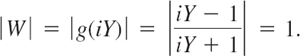
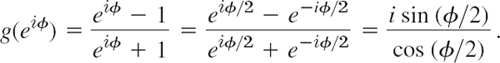
The right Z-half-plane is mapped inside this unit circle |W| = 1, not outside, because Z = 1 has its image g(1) = 0 inside that circle. Finally, the unit circle |z| = 1 is mapped onto the imaginary W-axis, because this circle is Z = eiø, so that (7) gives a pure imaginary expression, namely,
From the W-plane we get to the w-plane simply by a clockwise rotation through π/2; see (6).
Together we have shown that w = tan z maps S: −π/4 < Re z < π/4 onto the unit disk |w| < 1, with the four quarters of S mapped as indicated in Fig. 394. This mapping is conformal and one-to-one.
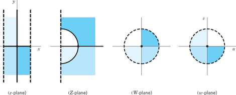
Fig. 394. Mapping by w = tan z
CONFORMAL MAPPING w = ez
- Find the image of x = c = const, −π < y π, under w = ez.
- Find the image of y = k = const, −∞ < x ∞, under w = ez.
3–7 Find and sketch the image of the given region under w = ez.
- 3.
 −π y π
 - 4. 0 < x < 1, < y < 1
- 5. −∞ < x < ∞, 0 y 2π
- 6. 0 < x < ∞, 0 < y < π/2
- 7. 0 < x < 1, 0 < y < π
- 8. CAS EXPERIMENT. Conformal Mapping. If your CAS can do conformal mapping, use it to solve Prob. 7. Then increase y beyond π, say, to 50π or 100π. State what you expected. See what you get as the image. Explain.
CONFORMAL MAPPING w = sin z
- 9. Find the points at which w = sin z is not conformal.
- 10. Sketch or graph the images of the lines x = 0, ±π/6, ±π/3, ±π/2 under the mapping w = sin z.
11–14 Find and sketch or graph the image of the given region under w = sin z.
- 11. 0 < x < π/2, 0 < y < 2
- 12. −π/4 < x < π/4, 0 < y < 1
- 13. 0 < x < 2π, 1 < y < 3
- 14. 0 < x < π/6, −∞ < y < ∞
- 15. Describe the mapping w = cosh z in terms of the mapping w = sin z and rotations and translations.
- 16. Find all points at which the mapping w = cosh 2πz is not conformal.
- 17. Find an analytic function that maps the region R bounded by the positive x- and y-semi-axes and the hyperbola xy = π in the first quadrant onto the upper half-plane. Hint. First map R onto a horizontal strip.
CONFORMAL MAPPING w = cos z
- 18. Find the images of the lines y = k = const under the mapping w = cos z.
- 19. Find the images of the lines x = c = const under the mapping w = cos z.
20–23 Find and sketch or graph the image of the given region under the mapping w = cos z.
- 20. 0 < x < 2π, < y < 1
- 21. 0 < x < π/2, 0 < y < 2 directly and from Prob. 11
- 22. −1 < x < 1, 0 y 1
- 23. π < x < 2π, y < 0
- 24. Find and sketch the image of the region 2 |z| 3, π/4 θ π/2 under the mapping w = Ln z.
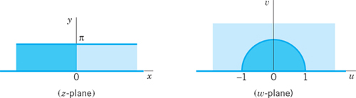
- 25. Show that
 maps the upper half-plane onto the horizontal strip 0 Im w π as shown in the figure.
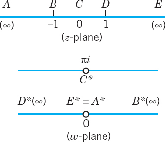
Problem 25
17.5 Riemann Surfaces. Optional
One of the simplest but most ingeneous ideas in complex analysis is that of Riemann surfaces. They allow multivalued relations, such as ![]() or w = ln z, to become single-valued and therefore functions in the usual sense. This works because the Riemann surfaces consist of several sheets that are connected at certain points (called branch points). Thus
or w = ln z, to become single-valued and therefore functions in the usual sense. This works because the Riemann surfaces consist of several sheets that are connected at certain points (called branch points). Thus ![]() will need two sheets, being single-valued on each sheet. How many sheets do you think w = ln z needs? Can you guess, by recalling Sec. 13.7? (The answer will be given at the end of this section). Let us start our systematic discussion.
will need two sheets, being single-valued on each sheet. How many sheets do you think w = ln z needs? Can you guess, by recalling Sec. 13.7? (The answer will be given at the end of this section). Let us start our systematic discussion.
The mapping given by
![]()
is conformal, except at z = 0, where w′ = 2z = 0. At z = 0, angles are doubled under the mapping. Thus the right z-half-plane (including the positive y-axis) is mapped onto the full w-plane, cut along the negative half of the u-axis; this mapping is one-to-one. Similarly for the left z-half-plane (including the negative y-axis). Hence the image of the full z-plane under w = z2 “covers the w-plane twice” in the sense that every w ≠ 0 is the image of two z-points; if z1 is one, the other is −z1. For example, z = i and −i are both mapped onto w = −1.
Now comes the crucial idea. We place those two copies of the cut w-plane upon each other so that the upper sheet is the image of the right half z-plane R and the lower sheet is the image of the left half z-plane L. We join the two sheets crosswise along the cuts (along the negative u-axis) so that if z moves from R to L, its image can move from the upper to the lower sheet. The two origins are fastened together because w = 0 is the image of just one z-point, z = 0. The surface obtained is called a Riemann surface (Fig. 395a). w = 0 is called a “winding point” or branch point. w = z2 maps the full z-plane onto this surface in a one-to-one manner.
By interchanging the roles of the variables z and w it follows that the double-valued relation
![]()
becomes single-valued on the Riemann surface in Fig. 395a, that is, a function in the usual sense. We can let the upper sheet correspond to the principal value of ![]() Its image is the right w-half-plane. The other sheet is then mapped onto the left w-half-plane.
Its image is the right w-half-plane. The other sheet is then mapped onto the left w-half-plane.
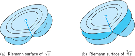
Similarly, the triple-valued relation ![]() becomes single-valued on the three-sheeted Riemann surface in Fig. 395b, which also has a branch point at z = 0.
becomes single-valued on the three-sheeted Riemann surface in Fig. 395b, which also has a branch point at z = 0.
The infinitely many-valued natural logarithm (Sec. 13.7)
![]()
becomes single-valued on a Riemann surface consisting of infinitely many sheets, w = Ln z corresponds to one of them. This sheet is cut along the negative x-axis and the upper edge of the slit is joined to the lower edge of the next sheet, which corresponds to the argument π < θ ![]() 3π, that is, to
3π, that is, to
![]()
The principal value Ln z maps its sheet onto the horizontal strip −π < v ![]() π. The function w = Ln z + 2πi maps its sheet onto the neighboring strip π < v
π. The function w = Ln z + 2πi maps its sheet onto the neighboring strip π < v ![]() 3π, and so on. The mapping of the points z ≠ 0 of the Riemann surface onto the points of the w-plane is one-to-one. See also Example 5 in Sec. 17.1.
3π, and so on. The mapping of the points z ≠ 0 of the Riemann surface onto the points of the w-plane is one-to-one. See also Example 5 in Sec. 17.1.
- If z moves from
 twice around the circle
  what does
  do?
do? - Show that the Riemann surface of w =
 has branch points at 1 and 2 sheets, which we may cut and join crosswise from 1 to 2. Hint. Introduce polar coordinates
  and
and  so that
- Make a sketch, similar to Fig. 395, of the Riemann surface of

4–10 RIEMANN SURFACES
Find the branch points and the number of sheets of the Riemann surface.
- 4.

- 5.

- 6. ln (6z − 2i)
- 7.

- 8.

- 9.

- 10.

CHAPTER 17 REVIEW QUESTIONS AND PROBLEMS
- What is a conformal mapping? Why does it occur in complex analysis?
- At what points are w = z5 − z and w = cos (πz2) not conformal?
- What happens to angles at z0 under a mapping w = f(z) if f′(z0) = 0, f″(z0) = 0, f′″(z0) ≠ 0?
- What is a linear fractional transformation? What can you do with it? List special cases.
- What is the extended complex plane? Ways of introducing it?
- What is a fixed point of a mapping? Its role in this chapter? Give examples.
- How would you find the image of x = Re z = 1 under w = iz, z2, ez, 1/z?
- Can you remember mapping properties of w = ln z?
- What mapping gave the Joukowski airfoil? Explain details.
- What is a Riemann surface? Its motivation? Its simplest example.
11–16 MAPPING w = z2
Find and sketch the image of the given region or curve under w = z2.
- 11. 1 < |z| < 2, |arg z| < π/8
- 12.

- 13. −4 < xy < 4
- 14. 0 < y < 2
- 15. x = −1, 1
- 16. y = −2, 2
17–22 MAPPING w = 1/z
Find and sketch the image of the given region or curve under w = 1/z.
- 17. |z| < 1
- 18. |z| < 1, 0 < arg z < π/2
- 19. 2 < |z| < 3, y > 0
- 20. 0 arg z π/4
- 21.
- 22. z = 1 + iy (−∞ < y < ∞)
23–38 LINEAR FRACTIONAL TRANSFORMATIONS (LFTs)
Find the LFT that maps
- 23. −1, 0, 1 onto 4 + 3i, 5i/2, 4 − 3i, respectively
- 24. 0, 2, 4 onto
 respectively
 - 25. 1, i, −i onto i, −1, 1, respectively
- 26. 0, 1, 2 onto 2i, 1 + 2i, 2 + 2i, respectively
- 27. 0, 1, ∞ onto ∞, 1, 0, respectively
- 28. −1, −i, i onto 1 −i, 2, 0, respectively
29–34 FIXED POINTS
Find the fixed points of the mapping
- 29. w = (2 + i)z
- 30. w = z4 + z − 64
- 31. w = (3z + 2)/(z − 1)
- 32. (2iz − 1)/(z + 2i)
- 33. w = z5 + 10z3 + 10z
- 34. w = (iz + 5)/(5z + i)
35–40 GIVEN REGIONS
Find an analytic function w = f(z) that maps
- 35. The infinite strip 0 < y < π/4 onto the upper half-plane v > 0.
- 36. The quarter-disk |z| < 1, x > 0, y > 0 onto the exterior of the unit circle |w| = 1.
- 37. The sector 0 < arg z < π/2 onto the region u < 1.
- 38. The interior of the unit circle |z| = 1 onto the exterior of the circle |w + 2| = 2.
- 39. The region x > 0, y > 0, xy < c onto the strip 0 < v < 1.
- 40. The semi-disk |z| < 2, y > 0 onto the exterior of the circle |w − π| = π.
SUMMARY OF CHAPTER 17 Conformal Mapping
A complex function w = f(z) gives a mapping of its domain of definition in the complex z-plane onto its range of values in the complex w-plane. If f(z) is analytic, this mapping is conformal, that is, angle-preserving: the images of any two intersecting curves make the same angle of intersection, in both magnitude and sense, as the curves themselves (Sec. 17.1). Exceptions are the points at which f′(z) = 0 (“critical points,” e.g. z = 0 for w = z2).
For mapping properties of ez, cos z, sin z etc. see Secs. 17.1 and 17.4.
Linear fractional transformations, also called Möbius transformations

(ad − bc ≠ 0) map the extended complex plane (Sec. 17.2) onto itself. They solve the problems of mapping half-planes onto half-planes or disks, and disks onto disks or half-planes. Prescribing the images of three points determines (1) uniquely.
Riemann surfaces (Sec. 17.5) consist of several sheets connected at certain points called branch points. On them, multivalued relations become single-valued, that is, functions in the usual sense. Examples. For ![]() we need two sheets (with branch point 0) since this relation is doubly-valued. For w = ln z we need infinitely many sheets since this relation is infinitely many-valued (see Sec. 13.7).
we need two sheets (with branch point 0) since this relation is doubly-valued. For w = ln z we need infinitely many sheets since this relation is infinitely many-valued (see Sec. 13.7).
1The general terminology is as follows. A mapping of a set A into a set B is called surjective or a mapping of A onto B if every element of B is the image of at least one element of A. It is called injective or one-to-one if different elements of A have different images in B. Finally, it is called bijective if it is both surjective and injective.
2ARTHUR CAYLEY (1821–1895), English mathematician and professor at Cambridge, is known for his important work in algebra, matrix theory, and differential equations.