Chapter 9. Beams on Elastic Foundations
9.1 Introduction
In the problems involving beams that we previously considered, support was provided at a number of discrete locations, and the beam was usually assumed to suffer no deflection at these points of support. We now explore the case of a prismatic beam supported continuously along its length by a foundation, which itself is assumed to experience elastic deformation. We shall take the reaction forces of the elastic foundation to be linearly proportional to the beam deflection at any point. This simple analytical model of a continuous elastic foundation is often referred to as the Winkler model.
The foregoing assumption not only leads to equations amenable to solution, but also represents an idealization closely approximating many real-world situations. Examples include a railroad track, where the elastic support consists of the cross ties, the ballast, and the subgrade; concrete footings on an earth foundation; long steel pipes resting on earth or on a series of elastic springs; ship hulls; and a bridgedeck or floor structure consisting of a network of closely spaced bars.
9.2 General Theory
Let us consider a beam on elastic foundation subject to a variable loading, as depicted in Fig. 9.1. The force q per unit length, resisting the displacement of the beam, is equal to −kυ. Here, υ is the beam deflection positive downward, as shown in the figure. The quantity k represents a constant, usually referred to as the modulus of the foundation, possessing the dimensions of force per unit length of beam per unit of deflection (for example, newtons per square meter or pascals).

Figure 9.1. Beam on an elastic (Winkler) foundation.
The analysis of a beam whose length is very much greater than its depth and width serves as the basis of the treatment of all beams on elastic foundations. Referring again to Fig. 9.1, which shows a beam of constant section supported by an elastic foundation, the x axis passes through the centroid, and the y axis is a principal axis of the cross section. The deflection υ, subject to reaction q and applied load per unit length p, for a condition of small slope, must satisfy the beam equation. Thus the first of Eqs. (5.32) becomes
EId4υdx4+kυ =p (9.1)
For those parts of the beam on which no distributed load acts, p = 0, and Eq. (9.1) takes the form
EId4υdx4+kυ =0(9.2)
We will consider only the general solution of Eq. (9.2), which requires the addition of a particular integral to satisfy Eq. (9.1) as well. Selecting υ=eax as a trial solution, we find that Eq. (9.2) is satisfied if
(α4+kEI)υ=0
This requires that
α=±β(1±i)
where
β=(k4EI)1/4(9.3)
The general solution of Eq. (9.2) may now be written as
υ=eβx[Acos βx+B sin βx]+e−βx[C cos βx+D sin βx](9.4)
where A, B, C, and D are the constants of integration.
In the discussion that follows, we first consider the case of a single load acting on an infinitely long beam. The solution of problems involving a variety of loading combinations will then rely on the principle of superposition.
9.3 Infinite Beams
Consider an infinitely long beam resting on a continuous elastic foundation, loaded by a concentrated force P (Fig. 9.2). As a real-world example, this situation might involve a train wheel exerting load P on the rail. The rail is supported by ties, ballast, and a road bed, which together are taken to act as an elastic foundation with modulus k. The variation of the reaction kυ is unknown, and the equations of static equilibrium are not sufficient for its determination. The problem is therefore statically indeterminate and requires additional formulation, which is available from the equation of the deflection curve of the beam.

Figure 9.2. Infinite beam on an elastic foundation carries a load at the origin: (a–e) loading, deflection, slope, bending moment, and shear diagrams, respectively.
Due to beam symmetry, only that portion to the right of the load P needs to be considered. The two boundary conditions for this segment are deduced from the fact that as x→ ∞, the deflection and all derivatives of υ with respect to x must vanish. On this basis, it is clear that the constants A and B in Eq. (9.4) must equal zero. What remains is
υ=e−βx(C cos βx+D sin βx)(9.5)
The conditions applicable at a very small distance to the right of P are
υ′(0)=0, V=−EIυ‴(0)=−P2(a)
where the minus sign is consistent with the general convention adopted in Section 1.3. Substitution of Eq. (a) into Eq. (9.5) yields
C=D=P8β3EI=Pβ2K
Introduction of the expressions for the constants into Eq. (9.5) provides the following equation, which is applicable to an infinite beam subject to a concentrated force P at midlength:
υ=Pβ2ke−βx(cos βx+sin βx)(9.6a)
or
υ=Pβ2ke−βx[√2sin(βx+π4)](9.6b)
As Equation (9.6b) clearly indicates, the characteristic of the deflection is an exponential decay of a sine wave of wavelength
λ=2πβ=2π(4EIk)1/4
To simplify the equations for deflection, rotation, moment, and shear, we introduce the following notations and relations:
f1(βx)=e−βx(cos βx+sin βx)f2(βx)=e−βxsin βx=−12βf′1f3(βx)=e−βx(cos βx−sin βx)=1βf′2=−12β2f″1f4(βx)=e−βxcos βx=−12βf′3=−12β2f′2=14β3f‴1f1(βx)=−1βf′4(9.7)
Table 9.1 lists numerical values of these functions for various values of the argument βx. The solution of Eq. (9.5) for specific problems is facilitated by this table and the graphs of the functions of βx [Ref. 9.1].
Table 9.1 Selected Values of the Functions Defined by Eqs. (9.7)
βx |
f1(βx) |
f2(βx) |
f3(βx) |
f4(βx) |
|---|---|---|---|---|
0 |
1 |
0 |
1 |
1 |
0.02 |
0.9996 |
0.0196 |
0.9604 |
0.9800 |
0.04 |
0.9984 |
0.0384 |
0.9216 |
0.9600 |
0.05 |
0.9976 |
0.0476 |
0.9025 |
0.9501 |
0.10 |
0.9907 |
0.0903 |
0.8100 |
0.9003 |
0.20 |
0.9651 |
0.1627 |
0.6398 |
0.8024 |
0.30 |
0.9267 |
0.2189 |
0.4888 |
0.7077 |
0.40 |
0.8784 |
0.2610 |
0.3564 |
0.6174 |
0.50 |
0.8231 |
0.2908 |
0.2415 |
0.5323 |
0.60 |
0.7628 |
0.3099 |
0.1431 |
0.4530 |
|
|
|
|
|
0.70 |
0.6997 |
0.3199 |
0.0599 |
0.3798 |
π/4 |
0.6448 |
0.3224 |
0 |
0.3224 |
0.80 |
0.6354 |
0.3223 |
−0.0093 |
0.3131 |
0.90 |
0.5712 |
0.3185 |
−0.0657 |
0.2527 |
1.00 |
0.5083 |
0.3096 |
−0.1108 |
0.1988 |
1.10 |
0.4476 |
0.2967 |
−0.1457 |
0.1510 |
1.20 |
0.3899 |
0.2807 |
−0.1716 |
0.1091 |
1.30 |
0.3355 |
0.2626 |
−0.1897 |
0.0729 |
1.40 |
0.2849 |
0.2430 |
−0.2011 |
0.0419 |
1.50 |
0.2384 |
0.2226 |
−0.2068 |
0.0158 |
|
|
|
|
|
π/2 |
0.2079 |
0.2079 |
−0.2079 |
0 |
1.60 |
0.1959 |
0.2018 |
−0.2077 |
−0.0059 |
1.70 |
0.1576 |
0.1812 |
−0.2047 |
−0.0235 |
1.80 |
0.1234 |
0.1610 |
−0.1985 |
−0.0376 |
1.90 |
0.0932 |
0.1415 |
−0.1899 |
−0.0484 |
2.00 |
0.0667 |
0.1231 |
−0.1794 |
−0.0563 |
2.20 |
0.0244 |
0.0896 |
−0.1548 |
−0.0652 |
3π/4 |
0 |
0.0670 |
−0.1340 |
.0.0670 |
2.40 |
−0.0056 |
0.0613 |
−0.1282 |
−0.0669 |
2.60 |
−0.0254 |
0.0383 |
−0.1019 |
−0.0636 |
|
|
|
|
|
2.80 |
−0.0369 |
0.0204 |
−0.0777 |
−0.0573 |
3.00 |
−0.0423 |
0.0070 |
−0.0563 |
−0.0493 |
π |
−0.0432 |
0 |
−0.0432 |
−0.0432 |
3.20 |
−0.0431 |
−0.0024 |
−0.0383 |
−0.0407 |
3.40 |
−0.0408 |
−0.0085 |
−0.0237 |
−0.0323 |
3.60 |
−0.0366 |
−0.0121 |
−0.0124 |
−0.0245 |
3.80 |
−0.0314 |
−0.0137 |
−0.0040 |
−0.0177 |
5π/4 |
.0.0279 |
.0.0139 |
0 |
.0.0139 |
4.00 |
−0.0258 |
−0.0139 |
0.0019 |
−0.0120 |
4.50 |
−0.0132 |
−0.0108 |
0.0085 |
−0.0023 |
|
|
|
|
|
3π/2 |
.0.0090 |
.0.0090 |
.00090 |
0 |
5.00 |
−0.0046 |
−0.0065 |
0.0084 |
0.0019 |
7π/4 |
0 |
.0.0029 |
0.0058 |
0.0029 |
6.00 |
0.0017 |
−0.0007 |
0.0031 |
0.0024 |
2π |
0.0019 |
0 |
0.0019 |
0.0019 |
6.50 |
0.0018 |
0.0003 |
0.0012 |
0.0018 |
7.00 |
0.0013 |
0.0006 |
0.0001 |
0.0007 |
9π/4 |
0.0012 |
0.0006 |
0 |
0.0006 |
7.50 |
0.0007 |
0.0005 |
−0.0003 |
0.0002 |
5π/2 |
0.0004 |
0.0004 |
.0.0004 |
0 |
Equation (9.6) and its derivatives, together with Eq. (9.7), yield the following expressions for deflection, slope, moment, and shearing force:
υ=Pβ2kf1θ=υ′=−Pβ2kf2M=EIυ″=−P4βf3V=−EIυ‴=−P2f4(9.8)
These expressions are valid for x ≥ 0. Based on the symmetry conditions:υ(–x) = υ(x), θ(–x) = –θ(x), M(–x) = M(x), and V(–x) = –V(x), the foregoing quantities are sketched versus βx in Figs. 9.2b–e.
From Fig. 9.2 (and Table 9.1), it is clear that the deflection, slope, moment, and shear all approach zero as β x becomes large. The beam deflection is zero at a distance 3π/(4β) from the load. The preceding results may thus be employed as approximations for beams of finite length
L=3π2β(b)
when loaded at the center. Equations (9.8) also give reasonable approximate results for very long beams for any location of the concentrated load inasmuch as the distance from the load to either end of the beam is equal or greater than 3π/(4β).
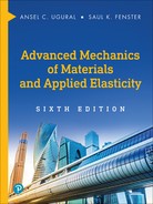
Example 9.1 Long Beam with a Partial Uniform Load
A very long rectangular beam of width 0.1 m and depth 0.15 m (Fig. 9.3) is subject to a uniform loading over 4 m of its length of p = 175 kN/m. The beam is supported on an elastic foundation having a modulus k = 14 MPa. Derive an expression for the deflection at an arbitrary point Q within length L. Find: the maximum deflection and the maximum force per unit length between beam and foundation. Use E = 200 GPa.
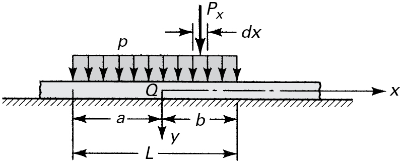
Figure 9.3. Example 9.1. Uniformly distributed load segment on an infinite beam on an elastic foundation.
Solution The deflection Δυ at point Q due to the load Px = p dx is, from Eq. (9.8),
Δυ=p dx2kβe−βx(cosβx+sinβx)
The deflection at point Q resulting from the entire distributed load is then
υQ=∫a0p dx2kβe−βx(cosβx+sinβx)+∫p dx2kβe−βx(cosβx+sinβx)b0 =p2k(2−e−βacosβa−e−βbcosβb)
or
υQ=p2k[2−f4(βa)−f4(βb)](c)
Although the algebraic sign of the distance a in Eq. (c) is negative, in accordance with the placement of the origin in Fig. 9.3, we will treat it as a positive number because Eq. (9.8) gives the deflection for positive x only. This approach is justified on the basis that the beam deflection under a concentrated load is the same at equal distances from the load, whether these distances are positive or negative. By the use of Eq. (9.3),
β=(k4EI)1/4 =(14×1064×200×109×0.1×0.153/12)1/4=0.888 m−1
From this value of β, βL = (0.888)(4) = 3.552 = β(a+b). We are interested in the maximum deflection, so we locate the origin at point Q, the center of the distributed loading. Now a and b represent equal lengths, so βa = βb = 1.776, and Eq. (b) gives
υmax=1752(14,000)[2−(−0.0345)−(−0.0345)]=0.0129 m
The maximum force per unit of length between beam and foundation is then kυmax = 14×106(0.0129) = 180.6 kN/m.
Example 9.2 Long Beam with a Moment
A very long beam is supported on an elastic foundation and is subjected to a concentrated moment Mo (Fig. 9.4). Determine the equations describing the deflection, slope, moment, and shear.

Figure 9.4. Example 9.2. Infinite beam resting on an elastic foundation subjected to Mo.
Solution Observe that the couple P · e is equivalent to Mo for the case in which e approaches zero (indicated by the dashed lines in the figure). Applying Eq. (9.8), we therefore have
υ=Pβ2k{f1(βx)−f1[β(x+e)]}=−Moβ2kf1[β(x+e)]−f1(βx)e =−Moβ2klime→0f1[β(x+e)]−f1(βx)e=−Moβ2kdf1(βx)dx=−Moβ2kf2(βx)
Successive differentiation yields
υ=Mokβ2f2(βx)θ=Mokβ3f3(βx)M=EIυ″=−Mo2f4(βx)V=−EIυ‴=−Moβ2f1(βx)(9.9)
which are the deflection, slope, moment, and shear, respectively.
9.4 Semi-Infinite Beams
In this section, we apply the theory developed in Section 9.3 to a semi-infinite beam, having one end at the origin and the other end extending indefinitely in a positive x direction, as depicted in Fig. 9.5. At x = 0, the beam is subjected to a concentrated load P and a moment MA. The constants C and D of Eq. (9.5) can be ascertained by applying the following conditions at the left end of the beam:
EIυ″=MA, EIυ‴=−V=P

Figure 9.5. Semi-infinite end-loaded beam on an elastic foundation.
The results are
C=P+βMA2β3EI, D=−MA2β2EI
The deflection is now found by substituting C and D into Eq. (9.5) as follows:
υ=e−βx2β3EI[Pcosβx+βMA(cosβx−sinβx)](9.10)
At x = 0,
δ=υ(0)=2βk(P+βMA)(9.11)
Finally, successively differentiating Eq. (9.10) yields expressions for slope, moment, and shear:
υ=2βk[Pf4(βx)+βMAf3(βx)]θ=−2β2k[Pf1(βx)+2βMAf4(βx)]M=Pβf2(βx)+MAf1(βx)V=−Pf3(βx)+2βMAf2(βx)(9.12)
Application of these equations together with the principle of superposition permits the solution of more complex problems, as illustrated next.
Example 9.3 Semi-Infinite Beam with a Concentrated Load Near Its End
Determine the equation of the deflection curve of a semi-infinite beam on an elastic foundation loaded by concentrated force P a distance c from the free end (Fig. 9.6a).
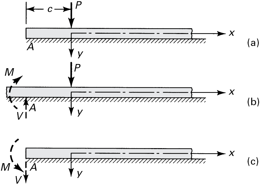
Figure 9.6. Example 9.3. Semi-infinite beam on an elastic foundation under load P.
Solution The problem may be restated as the sum of the cases shown in Figs. 9.6b and c. Applying Eqs. (9.8) and the conditions of symmetry, the reactions appropriate to the infinite beam of Fig. 9.6b are
M=−P4βf3(βc)V=−P2f4(βc)(a)
Superposition of the deflections of Fig. 9.6b and c [see Eqs. (9.8) and (9.12)] results in
υ=υinf+υsemi−inf=Pβ2kf1(βx)+2βk{−Vf4[β(x+c)]+βMf3[β(x+c)]}
Introducing Eqs. (a) into this equation, we obtain the following expression for deflection, which is applicable for positive x:
υ=Pβ2kf1(βx)+Pβk{f4(βc)f4[β(x+c)]−12f3(βc)f3[β(x+c)]}
This is clearly applicable for negative x as well, provided that x is replaced by |x|.
Example 9.4 Semi-Infinite Beam Loaded at Its End
A 2-m-long steel bar (E = 210 GPa) of 75-mm by 75-mm square cross section rests with a side on a rubber foundation (k = 24 MPa). If a concentrated load P = 20 kN is applied at the left end of the beam (Fig. 9.5), find: (a) the maximum deflection and (b) the maximum bending stress.
Solution Applying Eq. (9.3), we have
β=(k4EI)1/4=[24(106)4(210×109)(0.075)4 / 12]1/4=1.814 m−1
Given that βL = 1.814(2) = 3.638 > 3, the beam can be considered to be a long beam (see Section 9.5). Thus, Eqs. (9.12) with MA = 0 apply.
a. The maximum deflection occurs at the left end, for which f4(βx) is a maximum or βx = 0. The first of Eqs. (9.12) is therefore
υmax=2Pβk=2(20×103)(1.814)24(106)=3.02 mm
b. Referring to Table 9.1, f2(βx) has its maximum of 0.3224 at βx = π/4. Using the third of Eqs. (9.12),
Mmax=Pf2β=20(103)(0.3224)1.814=3.55 kN⋅m
The maximum stress in the beam is obtained from the flexure formula:
σmax=MmaxcI=3.55(103)(0.0375)(0.075)4 / 12=50.49 MPa
The location of this stress is at x = π/4β = 433 mm from the left end.
9.5 Finite Beams
Problems involving the bending of a finite beam on an elastic foundation may also be treated by applying the general solution, Eq. (9.4). In this instance, four constants of integration must be evaluated. To accomplish this, two boundary conditions at each end may be applied, which usually leads to rather lengthy formulations. Results have been obtained and tabulated for numerous cases using this approach.*
*For a detailed presentation of a number of practical problems, see Refs. 9.1 through 9.3.
An alternative approach to the solution of problems of finite beams with simply supported and clamped ends employs equations derived for infinite and semi-infinite beams, together with the principle of superposition. The use of this method was demonstrated in connection with semi-inverse beams in Example 9.3. Energy methods can also be employed in the analysis of beams whose ends are subjected to any type of support conditions. Solution by trigonometric series results in formulas that are particularly simple, as will be seen in Examples 10.13 and 11.6. Design tables for short beams with free ends on elastic foundation have been provided by Iyengar and Ramu [Ref. 9.4].
Let us consider a finite beam on an elastic foundation, centrally loaded by a concentrated force P (Fig. 9.7). We will compare the deflections occurring at the center and end of the beam. Note that the beam deflection is symmetrical with respect to C. The appropriate boundary conditions are, for x ≥ 0, υ′(L/2) = 0, EIυ‴(L/2) = P/2, EIυ″(0) = 0, and EIυ‴(0)=0. Substituting these conditions into the proper derivatives of Eq. (9.4) leads to four equations with unknown constants A, B, C, and D.
Figure 9.7. Comparison of the center and end deflections of a finite beam on an elastic foundation subjected to a concentrated center load.
After routine but somewhat lengthy algebraic manipulation, the following expressions are determined:
υC=2Pβ2k2+ cos βL+cosh βL / 2sin βL+sinh βL(9.13)
υE=2Pβkcos(βL / 2)cosh(βL / 2)sin βL+sinh βL(9.14)
From Eqs. (9.13) and (9.14), we have
υEυC=4cos(βL / 2)cosh(βL / 2)2+ cos βL+ cosh βL(9.15)
This result is sketched in Fig. 9.7.
9.6 Classification of Beams
The plot of Eq. (9.15) permits the establishment of a stiffness criterion for beams resting on an elastic foundation. It also helps us readily discern a rationale for the classification of beams on an elastic foundation. Referring to Fig. 9.7, the following groupings are possible:
Short beams, βL < 1: Inasmuch as the end deflection is essentially equal to that at the center, the deflection of the foundation can be determined to good accuracy by regarding the beam as infinitely rigid.
Intermediate beams, 1 < βL < 3: In this region, the influence of the central force at the ends of the beam is substantial, and the beam must be treated as finite in length.
Long beams, βL > 3: It is clear from the figure that the ends are not affected appreciably by the central loading. Therefore, if we are concerned with one end of the beam, the other end or the middle may be regarded as being an infinite distance away; that is, the beam may be treated as infinite in length.
These conditions do not relate only to the special case of loading shown in Fig. 9.7, but rather are quite general. Should greater accuracy be required, the upper limit of group 1 may be placed at βL = 0.6 and the lower limit of group 3 at βL = 5.
9.7 Beams Supported by Equally Spaced Elastic Elements
If a long beam is supported by individual elastic elements, as shown in Fig. 9.8a, the problem becomes simplified if the separate supports are replaced by an equivalent continuous elastic foundation. To accomplish this, it is assumed that the distance a between each support and the next support is small, and that the concentrated reactions Ri = Kυi are replaced by equivalent uniform or stepped distributed forces shown by the dashed lines of Fig. 9.8b, where K represents a spring constant (for example, newtons per meter).
For practical calculations, the usual limitation of the spring spacing is
a≤π4β(a)
The average continuous reaction force distribution is shown by the solid line in Fig. 9.8b. The intensity of the latter distribution is ascertained as follows:
Ra=Kaυ=q
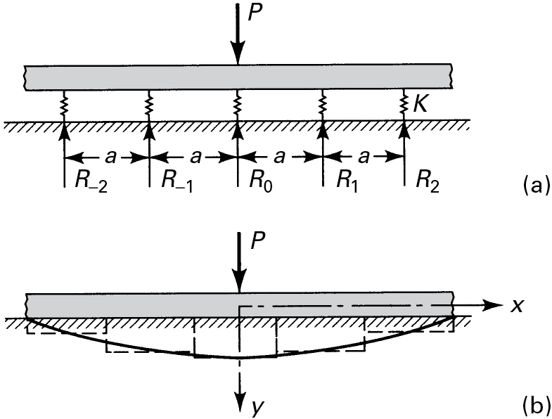
Figure 9.8. Infinite beam supported by equally spaced elastic springs. Loading diagram: (a) with concentrated reactions; (b) with average continuous reaction force distribution.
or
q=kυ(b)
where the foundation modulus of the equivalent continuous elastic support is
k=Ka(9.16)
The solution for the case of a beam on individual elastic support is then obtained through the use of Eq. 9.2, in which the value of k is that given by Eq. (9.16).
Example 9.5 Finite-Length Beam with a Concentrated Load
Supported by Springs
A series of springs, spaced so that a = 1.5 m, supports a long thin-walled steel tube having E = 206.8 GPa. A weight of 6.7 kN acts down the midlength of the tube. The average diameter of the tube is 0.1 m, and the moment of inertia of its section is 6 × 10⁻⁶ m4. Take the spring constant of each support to be K = 10 kN/m.
Find: The maximum moment and the maximum deflection, assuming negligible tube weight.
Solution Applying Eqs. (9.3) and (9.16), we obtain
k=Ka=10,0001.5=6667 Paβ=(66674×206.8×109×6×10−6)1/4=0.1914 m−1
The spacing of the springs, a < π/4β = 4.103 m, is correct. From Eq. (9.8), we have
σmax=McI=Pc4βI=6700×0.054×0.1914×6×10−6=72.93 MPaυmax=Pβ2k=6700×0.19142×6667=96.2 mm
9.8 Simplified Solutions for Relatively Stiff Beams
Examination of the analyses of the previous sections and of Fig. 9.7 leads us to conclude that the distribution of force acting on the beam by the foundation is, in general, a nonlinear function of the beam length coordinate. This distribution approaches linearity as the beam length decreases or as the beam becomes stiffer. Reasonably good results can be expected, therefore, by assuming a linearized elastic foundation pressure for stiff beams. The foundation pressure is then predicated on beam displacement in the manner of a rigid body [Ref. 9.5], and the reaction is, as a consequence, statically determinate.
To illustrate the approach, consider once more the beam of Fig. 9.7, this time with a linearized foundation pressure (Fig. 9.9). Because of loading symmetry, the foundation pressure is, in this case, not only linear but also constant. We will compare the results obtained in this case with those found earlier.
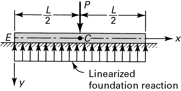
Figure 9.9. Relatively stiff finite beam on an elastic foundation and loaded at the center.
The exact theory states that points E and C deflect in accordance with Eqs. (9.13) and (9.14). The relative deflection of these points is simply
υ=υC−υE(a)
For the simplified load configuration shown in Fig. 9.9, the relative beam deflection may be determined by considering the elementary solution for a beam subjected to a uniformly distributed loading and a concentrated force. For this case, we label the relative deflection υ1 as follows:
υ1=PL348EI−5(P / L)L4384EI=PL3128EI(b)
The ratio of the relative deflections obtained by the exact and approximate analyses now serves to indicate the validity of the approximations. Consider
υυ1=32(βL)312cosh βL+ 12cosh βL+ 1−2 cosh 12 β Lcos12βLsinh βL+sin βL(c)
where υ and υ1 are given by Eqs. (a) and (b). The trigonometric and hyperbolic functions may be expanded as follows:
sin βL=βL−(βL)33!+(βL)55!−(βL)77!+⋯cos βL=1−(βL)22!+(βL)44!−(βL)66!+⋯sin βL=βL+(βL)33!+(βL)55!+⋯cosh βL=1+(βL)22!+(βL)44!+⋯(d)
Introducing these expressions into Eq. (c), we obtain
υυ1=1−23120(βL)44!+5120(βL)38!+⋯(e)
Substituting various values of βL into Eq. (e) discloses that, for βL < 1.0, υ/υ1 differs from unity by no more than 1%, and the linearization is seen to yield good results. It can be shown that for values of βL < 1, the ratio of the moment (or slope) obtained by the linearized analysis to that obtained from the exact analysis differs from unity by less than 1%.
Analysis of a finite beam, centrally loaded by a concentrated moment, also reveals results similar to those given here. We conclude that when βL is small (less than 1.0) no significant error is introduced by assuming a linear distribution of foundation pressure.
9.9 Solution by Finite Differences
Because of the considerable time and effort required in the analytical solution of practical problems involving beams on elastic foundations, approximate methods employing numerical analysis are frequently applied. A solution utilizing the method of finite differences is illustrated in the next example.
Example 9.6 Finite Beam Under Uniform Loading
Determine the deflection of the built-in beam on an elastic foundation, shown in Fig. 9.10a. The beam is subjected to a uniformly distributed loading p and is simply supported at x = L.

Figure 9.10. Example 9.6. (a) Uniformly loaded beam on an elastic foundation; (b) deflection curve for m = 2; (c) deflection curve for m = 3.
Solution The deflection is governed by Eq. (9.1), for which the applicable boundary conditions are
υ(0)=υ(L)=0, υ′(0)=0, υ″(L)=0(a)
The solution will be obtained by replacing Eqs. (9.1) and (a) by a system of finite difference equations. It is convenient to first transform Eq. (9.1) into dimensionless form through the introduction of the following quantities:
z=xL, ddx=1Lddz, at x=0, z=0; x=L, z=1
The deflection equation is therefore
EId4υdz4+kL4υ=pL4(b)
We next divide the interval of z(0, 1) into n equal parts of length h = 1/m, where m represents an integer. Multiplying Eq. (b) by h4 = 1/m4, we have
h4d4υdz4+kL4m4EIυ=pL4m4EI(c)
When we employ Eq. (7.23), Eq. (c) assumes the following finite difference form:
υn−2−4υn−1+6υn−4υn+1+υn+2+kL4m4EIυn=pL4m4EI(d)
Upon setting C = kL4/EI, this becomes
υn−2−4υn−1+[Cm4+6]υn−4υn+1+υn+2=pL4m4EI(e)
The boundary conditions, Eqs. (a), are transformed into difference conditions by employing Eq. (7.4):
υ0=0, υ−1=υ1, υn=0, υn−1=−υn+1(f)
Equations (e) and (f) represent the set required for a solution, where the degree of accuracy increases as the magnitude of m increases. Any desired accuracy can thus be attained.
For purposes of illustration, let k = 2.1 MPa, E = 200 GPa, I = 3.5 × 10⁻⁴ m4, L = 3.8 m, and p = 540 kN/m. Determine the deflections for m = 2, m = 3, and m = 4. Equation (e) becomes
υn−2−4υn−1+6(m4+1m4)υn−4υn+1+υn+2=1.6m4(g)
For m = 2, the deflection curve satisfying Eq. (f) is sketched in Fig. 9.10b. At z = ½, we have υn = υ1. Equation (g) then yields
υ1−4(0)+624+124υ1−4(0)−υ1=1.624
from which υ1 = 16 mm.
For m = 3, the deflection curve satisfying Eq. (f) is now that depicted in Fig. 9.10c. Hence, Eq. (g) at z=13 (by setting υn = υ1) and at z=23 (by setting υn = υ2) leads to
υ1+634+134υ1−4υ2=1.634−4υ1+634+134υ2−υ2=1.634
Solving, υ1 = 9 mm and υ2 = 11 mm.
For m = 4, a similar procedure yields υ1 = 5.3 mm, υ2 = 9.7 mm, and υ3 = 7.5 mm.
9.10 Applications
The theory developed for beams on an elastic foundation is applicable to many problems of practical importance, including that discussed in Section 9.10.1. The concept of a beam on an elastic foundation may also be employed to approximate stress and deflection in axisymmetrically loaded cylindrical shells (to be discussed in Chapter 13). The governing equations of the two problems are of the same form, which means that solutions of one problem become solutions of the other problem through a simple change of constants [Ref. 9.6].
9.10.1 Grid Configurations of Beams
The ability of a floor to sustain extreme loads without undue deflection, as in a machine shop, is significantly enhanced by combining the floor beams in a particular array or grid configuration. Usually, this configuration consists of two systems of equally spaced perpendicular beams, mutually perpendicular and attached rigidly at the point of intersection.
Such a design is illustrated in Case Study 9.1. Interestingly, similarly grid configuration of curved beams forms a typical flight structure.
Case Study 9.1 Analysis of Machine Room Floor
A single concentrated load P acts at the center of a machine room floor composed of 79 transverse beams (spaced a = 0.3 m apart) and one longitudinal beam, as shown in Fig. 9.11. If all beams have the same modulus of rigidity EI, determine the deflection and the distribution of load over the various transverse beams supporting the longitudinal beam. Assume that the transverse and longitudinal beams are attached so that they deform together.
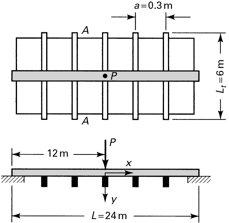
Figure 9.11. Case Study 9.1. Long beam supported by several identical and equally spaced crossbeams. All beams are simply supported at their ends.
Solution The spring constant K of an individual elastic support such as beam AA is
K=RCυC=RCRCL3t / 48EI=48EIL3t
where υc the central deflection of a simply supported beam of length Lt carrying a center load RC. From Eq. (9.16), the modulus k of the equivalent continuous elastic foundation is found to be
k=Ka=48EIaL3t
Thus,
β=4√k4EI=4√12aL3t=3.936Lt
and
βL=3.936Lt(4Lt)=15.744, βa=3.936LtLt20=0.1968
In accordance with the criteria discussed in Sections 9.4 and 9.5, the longitudinal beam may be classified as a long beam resting on a continuous elastic support of modulus k. Consequently, from Eqs. (9.8), the deflection at midspan is
υP=Pβ2k(1)=3.936P2LtaL3t48EI=1.968PL2ta48EI(a)
The deflection of a transverse beam depends on its distance x from the center of the longitudinal beam, as shown in the following table:
x |
0 |
2a |
4a |
6a |
8a |
10a |
12a |
16a |
20a |
24a |
|---|---|---|---|---|---|---|---|---|---|---|
f1(βx) |
1 |
0.881 |
0.643 |
0.401 |
0.207 |
0.084 |
−0.0002 |
−0.043 |
−0.028 |
−0.009 |
υ |
υp |
0.88 υp |
0.643υp |
0.401υp |
0.20υp |
0.084υp |
−0.0002υp |
−0.043υp |
−0.028υp |
−0.009υp |
We are now in a position to calculate the load RCC supported by the central transverse beam. Since the midspan deflection υM of the central transverse beam is equal to υP. Hence,
υM=RCCL3t48EI=1.968PL2ta48EI
and
RCC=1.968PaLt=0.0984P(b)
The remaining transverse beam loads are now readily calculated on the basis of the deflections in the table, recalling that the loads are linearly proportional to the deflections.
Comments Beginning with beam 12, it is possible for a transverse beam to be pulled up as a result of the central loading, as indicated by the negative value of the deflection. The longitudinal beam thus serves to decrease transverse beam deflection only if it is sufficiently rigid.
References
9.1. FLUGGE, W., ed. Handbook of Engineering Mechanics. New York: McGraw-Hill, 1968
9.2. HETENYI, M. Beams on Elastic Foundations. New York: McGraw-Hill, 1960.
9.3. TING, B. Y. Finite beams on elastic foundation with restraints. J. Struct. Div., Proc. Am. Soc. Civil Eng. 108(ST 3):611–621. March 1982.
9.4. IYENGAR, K. T., SUNDARA, R., and RAMU, S. A. Design Tables for Beams on Elastic Foundation and Related Problems. London: Applied Science Publications, 1979.
9.5. SHAFFER, B. W. Some simplified solutions for relatively simple stiff beams on elastic foundations. Trans. ASME J. Eng. Industry. 1–5, February 1963.
9.6. UGURAL, A. C. Plates and Shells: Theory and Analysis, 4th ed. Boca Raton, FL: CRC Press, Taylor & Francis Group, 2018.
Problems
Sections 9.1 through 9.4
9.1. A very long steel I-beam, 0.127 m deep, resting on a foundation for which k = 1.4 MPa, is subjected to a concentrated load at midlength. The flange is 0.0762 m wide, and the cross-sectional moment of inertia is 5.04 × 10⁻⁶ m4. What is the maximum load that can be applied to the beam without causing the elastic limit to be exceeded? Assume that E = 200 GPa and σyp = 210 MPa.
9.2. A long steel beam (E = 200 GPa) of depth 2.5b and width b is to rest on an elastic foundation (k = 20 MPa) and support a 40-kN load at its center (Fig. 9.2). Design the beam (compute b) if the bending stress is not to exceed 250 MPa.
9.3. Calculate the maximum deflection, maximum bending moment, and maximum stress in the steel (E = 210 GPa) I-beam of moment of inertia I = 40(106) mm4 subjected to a load P (Fig. 9.2). The distance from the top of the beam to its centroid is 100 mm. Given: P = 150 kN, k = 15 MPa.
9.4. A long wooden b × h rectangular beam rests on elastic foundation and carries a uniform load p over a region L (Fig. 9.3). Given: b = 90 mm, h = 180 mm, p = 40 kN/m, k = 5 MPa, L = 4 m, E = 12 GPa. Taking the origin of the coordinates at the center of the beam (a = b = L/2), calculate the maximum deflection.
9.5. A long beam on an elastic foundation is subjected to a sinusoidal loading p = p1 sin(2πx/L), where p1 and L are the peak intensity and wavelength of loading, respectively. Determine the equation of the elastic deflection curve in terms of k and β.
9.6. If point Q is taken to the right of the loaded portion of the beam shown in Fig. 9.3, what is the deflection at this point?
9.7. A single train wheel exerts a load of 135 kN on a rail assumed to be supported by an elastic foundation. For a modulus of foundation k = 16.8 MPa, find: the maximum deflection and maximum bending stress in the rail. The respective values of the section modulus and modulus of rigidity are S = 3.9 × 10⁻⁴ m3 and EI = 8.437 MN ⋅ m2.
9.8. Re-solve Prob. 9.1 based on a safety factor of n = 2.5 with respect to yielding of the beam and using the modulus of foundation of k = 12 MPa.
9.9. An infinite 6061-T6 aluminum alloy beam of b × b square cross section resting on an elastic foundation of k carries a concentrated load P at its center (Fig. 9.2). Using a factor of safety of n with respect to yielding of the beam, compute the allowable value of b. Given: E = 70 GPa, σyp = 260 MPa (Table D.1), k = 7 MPa, P = 50 kN, and n = 1.8.
9.10. Re-solve Prob. 9.7 for the case in which a single train wheel exerts a concentrated load of P = 250 kN on a rail resting on an elastic foundation having k = 15 MPa.
9.11. A long rail is subjected to a concentrated load at its center (Fig. 9.2). Determine the effect on maximum deflection and maximum stress of overestimating the modulus of foundation k by (a) 25% and (b) 40%.
9.12. Calculate the maximum resultant bending moment and deflection in the rail of Prob. 9.7 if two wheel loads spaced 1.66 m apart act on the rail. The remaining conditions of the problem are unchanged.
9.13. Determine the deflection at any point Q under the triangular loading acting on an infinite beam on an elastic foundation (Fig. P9.13).
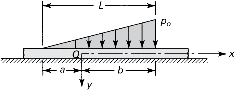
Figure P9.13.
9.14. What are the reactions acting on a semi-infinite beam built in at the left end and subjected to a uniformly distributed loading p? Use the method of superposition. (Hint: At a large distance from the left end, the deflection is p/k.)
9.15. A semi-infinite beam on an elastic foundation is subjected to a moment MA at its end (Fig. 9.5 with P = 0). Find: (a) the ratio of the maximum upward and maximum downward deflections and (b) the ratio of the maximum and minimum moments.
9.16. A semi-infinite beam on an elastic foundation is hinged at the left end and subjected to a moment ML at that end. Determine the equation of the deflection curve, slope, moment, and shear force.
Sections 9.5 through 9.10
9.17. A machine base consists partly of a 5.4-m-long steel I-beam supported by coil springs spaced a = 0.625 m apart. The constant for each spring is K = 180 kN/m. The moment of inertia of the I-section is 5.4 × 10⁻⁶ m4, the depth is 0.127 m, and the flange width is 0.0762 m. Assuming that a concentrated force of 6.75 kN transmitted from the machine acts at midspan, determine the maximum deflection, maximum bending moment, and maximum stress in the beam.
9.18. An aluminum alloy, I-beam (depth h = 120 mm, I = 2.5 × 106 mm4, E = 70 GPa) of length L = 8.5 m is supported by 7 springs (K = 120 kN/m) spaced at a distance a = 1.2 m along the beam, as depicted in Fig. P9.18. Find the maximum deflection and maximum stress if the beam is under a concentrated center load P = 15 kN.
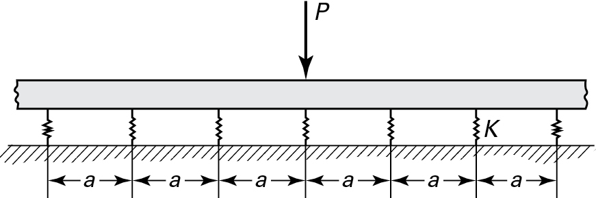
Figure P9.18.
9.19. A steel beam of 0.75-m length and 0.05-m square cross section is supported on three coil springs spaced a = 0.375 m apart. For each spring, K = 18 kN/m. Determine (a) the deflection of the beam if a load P = 540 N is applied at midspan and (b) the deflection at the ends of the beam if a load P = 540 N acts 0.25 m
from the left end.
9.20. A finite beam with EI = 8.4 MN ⋅ m2 rests on an elastic foundation for which k = 14 MPa. The length L of the beam is 0.6 m. If the beam is subjected to a concentrated load P = 4.5 kN at its midpoint, determine the maximum deflection.
9.21. A finite beam is subjected to a concentrated force P = 9 kN at its midlength and a uniform loading p = 7.5 kN/m. Find: the maximum deflection and slope if L = 0.15 m, EI = 8.4 MN ⋅ m2, and k = 14 MPa.
9.22. A finite beam of length L = 0.8 m and EI = 10 MN m resting on an elastic foundation (k = 8 MPa) is under a concentrated load P = 15 kN at its midlength. What is the maximum deflection?
9.23. A finite cast-iron beam of width b, depth h, and length L, resting on an elastic foundation of modulus k, is subjected to a concentrated load P at midlength and a uniform load of intensity p. Calculate the maximum deflection and the slope. Given: E = 70 GPa (Table D.1), b = 100 mm, h = 180 mm, L = 400 mm, P = 8 kN, p = 7 kN/m, and k = 20 MPa.
9.24. Re-solve Example 9.6 for the case in which both ends of the beam are simply supported.
9.25. Assume that all the data of Case Study 9.1 are unchanged except that a uniformly distributed load p replaces the concentrated force on the longitudinal beam. Compute the load RCC supported by the central transverse beam.