
4
DIGITAL CONTROL-SYSTEM ANALYSIS AND DESIGN
4.1. INTRODUCTION
This chapter is concerned with a class of feedback control systems in which the signal at one or more points appears as a train of pulses rather than as a continuous function. Such a system is known as a digital control system, in contrast to a continuous control system, where the signal is continuous everywhere. The controlling information, determined by the amplitude of the pulses, is present only at discrete instants of time, which in this chapter, are assumed to be equally spaced. Because of the inherent time delay introduced by the sampling operation, stabilization of the digital control system becomes a more complex problem than with continuous systems requiring special techniques for analysis and design.
Digital control systems are used in a wide variety of applications. The impetus for the use of this class of control systems has been the ready availability of digital computers, and the improvement in cost and reliability of digital computers. Digital control systems are very common today and are used in controlling robots [1], navigation systems for aircraft and ships, aircraft autopilots, mass transit vehicles, chemical process control systems, and automation systems for various applications.
There are several excellent books avail able on digital control systems that are dedicated to this subject only [2–5]. The purpose of this chapter is to present digital control systems to the student and the practicing engineer to a level permitting the analysis and design of digital control systems. We will extend the concepts developed in this book for the analysis and design of continuous control systems to digital control systems. We will focus attention in this chapter on that class of digital control systems where the digital computer is connected to the control elements and controlled system by means of analog-to-digital (A/D) and digital-to-analog (D/A) converters as illustrated in Figure 4.1. Therefore, this system contains both discrete signals [r(kT), e(kT), b(kT)], and continuous signals [u(t), m(t), c(t)]. A system having both discrete and continuous signals is defined as a sampled-data system [2].

Figure 4.1 A sampled-data system.
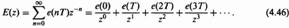
The sampling operation can best be described by considering a variable of interest, e(t), which is shown in Figure 4.2a. Let us assume that this function is sampled at equal intervals of time T, so that a sampled function can be described by the sequence of numbers given by
![]()
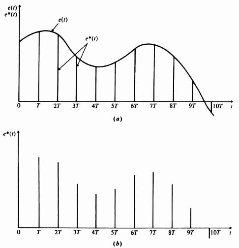
Figure 4.2 (a) Sampling a variable, e(t). (b) Sampled function, e*(t) = e(kT).
This resultant series of numbers, e(kT) gives a limited description of the function e(t). Specifically, the value of e(t) at times 0, T, 2T, 3T, 4T, and nT seconds are known. Its value at other times can only be approximated by means of interpolation techniques.
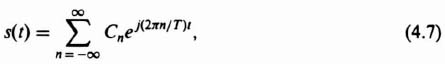
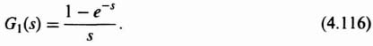
In practical control systems, it is necessary that the discrete data be reconstructed during the intervals between samples, because the controlled elements and controlled system components are continuous, or analog, type of devices. Data extrapolators, or predictors, are usually quite simple devices which predict values during sampling intervals based upon either the last one, two, or three pieces of data. Very rarely are more than three pieces of information used. Figure 4.2b illustrates the sampled information which will be designated as e*(t) or e(kT). It is common practice in sampled-data theory to denote the sampled version of time with an asterisk. Figure 4.3 illustrates the information after it is reconstructed by means of a simple holding device, which simply remembers the last piece of information until a new sample is obtained. This type of holding circuit is known as a zero-order hold. The reconstructed function is designated as eR(t).
This chapter discusses the basic concepts and characteristics of sampled-data systems and illustrates the techniques for analyzing and designing such systems. An analysis of the sampling process, data extrapolators, stability, and compensation techniques will be presented. In addition, the relations between variables of the control system will be obtained by use of a new transformation which is denoted as the z transformation. The use of the Laplace transformation in sampled-data control systems is quite cumbersome, because we are working with difference equations [2], rather than differential equations as in continuous systems. The transformation is very useful in the analysis and design of sampled-data control systems. Several practical design problems are presented for illustrative purposes wherever appropriate.
4.2. CHARACTERISTICS OF SAMPLING
We will analyze in this section the operation of an ideal sampler which produces a discrete-time signal from a continuous-time signal. For purposes of this analysis, let us consider the following sampler, which samples the continuous signal e(t) and produces the discrete-time signal e*(t):

Figure 4.3 Reconstruction of e*(t) by means of a zero-order hold.

We shall further assume that the closure of the switch is of very short duration as compared to the time between closures. Therefore, the value of the function at the output of the switch is the instantaneous values of the function e(t) when the switch is closed.
In order to obtain a clearer mathematical picture of the sampling process, we can think of the sampler as a device which multiplies some input intelligence signal e(t) by a sampling function s(t). This is mathematically equivalent to a modulation process where the sampling function represents the carrier that is being modulated by the input intelligence signal. This can be expressed as
From the viewpoint of mathematical simplicity, it is very desirable to define the sampling function as a series of unit impulses that are characterized by having an infinitely narrow width and an infinite amplitude. Its total area is defined as unity. However, practical samplers remain closed for a finite length of time and may result in an actual sampling pulse whose area may be a finite number A. For this case, the only modification that is necessary to the unit-impulse approximation is to replace the unit area impulse with one whose area is A. In practice, the only real requirement for using the unit-impulse approximation is that the sampling duration be small compared to the time constant of the system. This is usually the case, because feedback control systems generally represent low-pass filters. In the succeeding discussion, we shall assume that the sampling function is a series of unit impulses that can be expressed as

where δ(t − nT) represents an impulse having unit area at time t = nT.
The Laplace transform of the unit-impulse modulated function e*(t) can be easily determined. Assuming that the function e(t) is zero for negative time, then e*(t) can be expressed as

where e(nT) is the value of e(t) at the sampling instant nT, and δ(t − nT) represents a unit impulse occurring at the instant nT. The Laplsee transform of Eq. (4.3) can be written as

The Laplace transform for a sampler having equal sampling intervals and whose switching can be represented by a series of unit impulses is an infinite summation which can be expressed in closed form, This is easily demonstrated by considering the case where the function e(t) is a simple unit step, U(t). For this case, all values of e(nT) are equal to unity for positive time and zero for negative times. The Laplace transform of e*(t), given by Eq. (4.3), can be expressed as

Equation (4.5) is recognizable as a geometric progression in e−Ts, which can be expressed as

The Laplace transform for the unit-impulse sampling device can be obtained in another form, which makes use of the fact that the sampling function s(t) is periodic and can be expressed as a Fourier series. (Fourier series were reviewed in Section 2.3‡, and will also be used in Section 5.8 when we derive describing functions.) Expanding s(t) into a Fourier series, we get
where Cn represents the Fourier coefficients of the exponential series. These coefficients can be easily determined for the unit-impulse series from the integral

Because the area of any impulse equals unity, the integral also equals unity, and all of the Fourier coefficients can be expressed by
Substituting Eq. (4.9) into (4.7), we obtain the expression for the Fourier series of the sampling function:
The expression for the Fourier series of the sampled function, e*(t), can easily be obtained by substituting Eq. (4.10) into Eq. (4.1). The result is
Notice that the term 2π/T in the exponent of Eq. (4.11) represents the radian frequency of sampling and will be defined as ωs. Therefore e*(t) can be expressed as
The Laplace transform of Eq. (4.12) is given by [use was made of the frequency shifting theorem given by Eq. (2.72)‡]:
Let us now utilize Eq. (4.13) in order to determine E*(s) for the case where e(t) is a unit step. The result will then be compared with that obtained previously, given by Eq. (4.6). Because the Laplace transform of a unit step is 1/s, the Laplace transform of the sampled function is given by

Notice that Eq. (4.14) is an infinite summation and cannot be expressed in closed form as was Eq. (4.6). However, Eq. (4.14) does show very clearly the periodic properties of the Laplace transform of the sampled function. From Eq. (4.14), the frequency spectrum can be expressed as
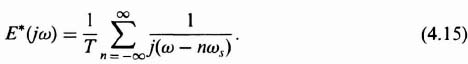
It appears that the spectrum is not band limited and exact reproduction of the sampled signal is not possible.
In general, the frequency spectrum of a sampled function can be expressed as
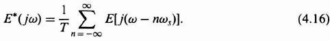
Notice that the frequency spectrum is periodic in ωs. If the input intelligence signal e(t) has a spectral distribution as shown in Figure 4.4, then the output of the sampler will have a frequency spectrum as shown in Figure 4.5. The bandwidth of the input signal is designated ωc.
At this point in our development of sampled data theory, the relation between ωc and ωs, will be considered. Referring to Figure 4.5, it can be seen that the function e(t) can be recovered if the sampled function, e*(t), is passed through an ideal low-pass filter as shown by the dashed line. Shannon [6] has shown that if the highest input frequency is ωc, then the sampling frequency must be at least 2ωc in order that the input function e(t) can be recovered undistorted. If the sampling frequency is less than 2ωc, then the spectral distribution from 0 to ωc would overlap partly the region from ωs to ωs − ωc. This would result in the filter recovering the input signal distorted by the overlapped portion of the first sideband (alias frequency), and aliasing occurs. Practical considerations often dictate a sampling frequency much higher than twice the highest input frequency. In addition, because signals generally do not have finite frequency spectrums and filters do not have ideal frequency response characteristics as shown by the dashed line in Figure 4.5, the recovered signal always has a certain amount of distortion. This distortion is referred to as ripple. It occurs at the sampling frequency and its harmonics should be treated as noise of the sampled-data control system.
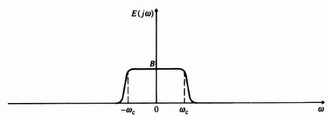
Figure 4.4 Input function frequency spectrum.
4.3. DATA EXTRAPOLATORS
A data extrapolator is a device that reconstructs a sampled function into a continuous signal based upon a knowledge of past samples. This device, which is also referred to as a data hold, follows the sampler in practical feedback control systems. Figure 4.6 illustrates a simple system having a sampler, data hold, and a process which is to be controlled. The reconstructed signal, eR(t), is piecewise continuous and is applied to the process.
Data extrapolators are classified according to the number of prior samples that are required for predicting the sampled function during waiting intervals. As was illustrated in Figure 4.3, an extrapolator which only depends on the value of the sampled function at the beginning of a sampling interval is known as a zero-order hold. It is similar in operation to an electronic clamping circuit that maintains its output level equal to the magnitude of an input pulse and then resets itself when a new pulse is applied. An extrapolator that depends on two prior samples is known as a first-order hold. Figure 4.7 illustrates a reconstructed time function eR(t) produced by such an extrapolation from a signal e(t). Practical systems usually do not use data extrapolators that are higher than first order, because they introduce an excessive phase lag into the feedback control system. In addition, they usually increase the effects of noise and are more complex and costly.
The transfer function of a zero-order hold can be easily determined from the impulsive response. This can be obtained from the superposition of a positive unit step at zero time and a negative unit step T seconds later, where T is the sampling period. This is illustrated in Figure 4.8. The impulsive response can be expressed in the time domain as
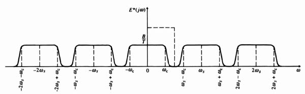
Figure 4.5 Sampled function frequency spectrum.

Figure 4.6 Simple sampled-data feedback control system.
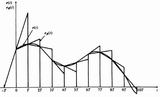
Figure 4.7 Reconstruction of a signal by means of a first-order hold.
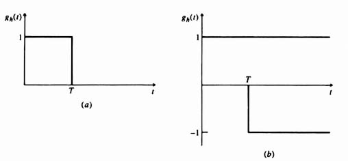
Figure 4.8 (a) Zero-order hold impulsive response. (b) Equivalent step-function components.
The Laplace transform of Eq. (4.17) is
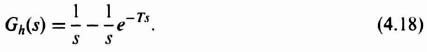
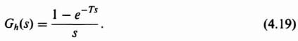
Equation (4.19) is quite useful for studying the effects of a zero-order hold in a feedback control system.
The frequency response of the zero-order hold can be expressed as

In order to obtain an expression for the amplitude and phase characteristics of a zero-order hold, Eq. (4.20) is rearranged successively as follows:
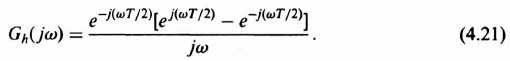
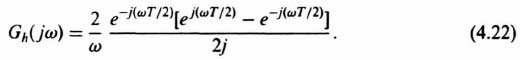
Observing that ![]() is equal to sin(ωT/2), Eq. (4.22) can be simplified to
is equal to sin(ωT/2), Eq. (4.22) can be simplified to
Multiplying numerator and denominator by T, a familiar sin x/x term results:

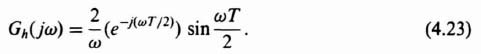
The amplitude and phase of Gh(jω) are sketched in Figure 4.9. The frequency characteristics of this extrapolating device are similar to that of a low-pass filter where full cutoff occurs at 2πn/T rad/sec, where n is an integer. Of primary concern to the control engineer is the phase shift introduced by the zero-order hold. This appreciable phase lag may cause a feedback system, which might ordinarily be stable in its continuous form, to become unstable.
Let us next determine the characteristics of a first-order holding device. Figure 4.7 shows that the extrapolated function of a first-order hold is linear and has a slope determined by the last two samples. The transfer function of such an extrapolating device can be obtained in a manner similar to that used for the zero-order hold. The impulsive response of a first-order hold is shown in Figure 4.10a. Its equivalent step and ramp function components are sketched in Figure 4.10b. By superposition the Laplace transform of the impulsive response can be expressed as


Figure 4.9 Amplitude and phase response of a zero-order hold.

Figure 4.10 (a) First-order hold impulsive response. (b) Equivalent step-and-ramp-function components.
This can be simplified to
Equation (4.26) is quite useful for studying the effects of a first-order hold in a feedback control system.
The frequency characteristics of the first-order hold can be expressed as
In order to obtain the amplitude and phase characteristics, Eq. (4.27) is rearranged as follows:

Observing that ![]() equals sin2(ωT/2), Eq. (4.28) can be simplfied to
equals sin2(ωT/2), Eq. (4.28) can be simplfied to

The amplitude and phase of Gh(jω) are sketched in Figure 4.11.
Observe that the amplitude response of this extrapolating device is similar to that of the zero-order hold. However, the phase shift introduced by the first-order hold is almost twice that of the zero-order hold. For example, at ω = 2π/T, the first-order hold introduces a phase shift of −2π + tan−1 2π(−279.04°), and the zero-order hold introduces a phase shift of −180°. This greatly affects the stability and is a serious disadvantage of the more complex extrapolator. In addition, the higher-order extrapolator transmits a greater amount of the higher-frequency components with a resultant higher noise level in the system. For these reasons, higher-order holding devices are not usually included in practical feedback control systems. Their only advantage is that they are capable of perfectly reproducing functions (in the steady state) which are higher-order derivatives of time. For example, a zero-order hold is only capable of reproducing a step function perfectly, while a first-order hold can reproduce a ramp function perfectly. However, the zero-order hold is adequate for most practical applications.
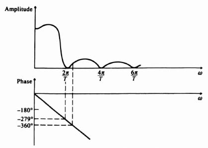
Figure 4.11 Amplitude and phase response of a first-order hold.
4.4. z-TRANSFORM THEORY
The analysis of continuous feedback control systems is considerably simplified by the use of the Laplace transform. The transfer function of simple networks and complicated processes can be represented by an algebraic function that is a ratio of two polynomials in s. A sampler, however, produces an equivalent transfer function which is the ratio of two polynomials in eTs. In Section 4.2, Eq. (4.4) showed this effect for the Laplace transform of e(t). This result stems from the fact that we are working with difference equations in sampled-data control systems instead of differential equations as in continuous systems. It is possible to obtain an algebraic relationship, similar in form to the Laplace transform, if eTs is replaced by some arbitrary symbol such as z. This is the basis of the z-transform theory [2–5]. The analysis of sampled-data control systems is very similar to that of continuous systems when the z-transform is employed.
The z transform of a sampler can be simply obtained by substituting z = eTs into Eq. (4.4). This results in a power series of 1/z as follows:
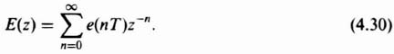
This definition of the z transform is denoted as the one-sided z transform, which assumes that e(t) = 0 for t < 0, or e(nT) = 0 for n < 0. Equation (4.30) results in terms that are negative powers of z−1, and it uniquely defines the z transform. For functions of e(t) that have values for −∞ < t < ∞, and for e(nT) that have values for n = 0, ±1, ±2, ±3,…, we use the two-sided z transform:
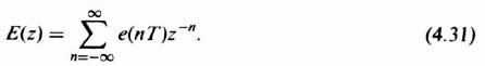
Equation (4.31) results in terms that contain both positive and negative powers of z. To uniquely define the z transform in this case, we must also define bounds on the magnitude of z for which Eq. (4.31) converges. Otherwise, it is possible for more than one sequence to have the same z transform. For example, let us consider the following two sequences:

Both of these sequences have the same z transform:
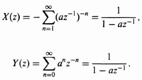
By also defining the region of convergence for X(z) to be

and the region of convergence for Y(z) to be
![]()
then the z transforms of X(z) and Y(z) converge and are unique definitions. As we are not interested in the practical world in functions which exist for negative times, we will only consider the one-sided z transform in this chapter.
Notice that the z transform describes the values of the time function at the sampling instants only. It offers no information on the behavior of the function between the sampled times.
In order to analyze or synthesize a feedback control system containing a sampler, it is also necessary to obtain the z transforms of all other elements in the closed loop. Stability can then be determined using the complex z-plane just as the complex s-plane (Nyquist diagram) was used in the case of continuous systems. For purposes of clarity, a brief comparison of the conditions for stability will next be made for these two planes.
We had concluded from Eqs. (4.14)–(4.16) that the frequency spectrum of a sampled function is periodic in s with period jωs. Therefore, it is important to recognize that if a function E(s) has a pole (zero) at s = sa, then E*(s) has poles (zeros) at s = sa + jnωs, where n = 0. ±1, ±2,…, ±∞. Therefore, for every pole (or zero) at s = sa in the s-plane, the sampled function E*(s) has the same value at all periodic frequency points sa + jnωs, where n is an integer. Figure 4.12 illustrates a periodic function E*(s), where E(s) has a pole (designated as X) at s = sa = −σa + jωa and the sampling operation generates a pole in E*(s) at −σa + j(ωa + nωs) where n is an integer. In practice, because the low-pass filter characteristics of the process and the zero-order hold (or first-order hold) greatly attenuate the response of the poles and zeros in the complementary strips, we will only consider the poles and zeros in the major strip for analysis and design in this chapter.
Let us focus attention on the primary strip of the s-plane shown in Figure 4.13a. We wish to map the contour S – T – U – V – W of the primary strip in the s-plane into the z-plane. Using the definition of the z transform, we can obtain the necessary relationship as follows:

Figure 4.12 Location of a complex pole E(s) at −σa + jωa (labeled X) in the primary strip, and the location of additional poles of E*(s), caused by sampling, in the complementary strips.
The results are shown in Figure 4.13b, and the corresponding sequence of points S–T–U–V–W–S in the s-plane and z-planes are illustrated. It is important to recognize that because the area of any complementary strip in the s-plane is mapped into the same unit circle in the z-plane, the correspondence between the s- and z-planes is not unique. Therefore, a single point on the z-plane corresponds to an infinite number of points in the s-plane. However, a single point in the s-plane corresponds to a single point in the z-plane.
We can now reach a very important conclusion regarding stability in the z-plane. Because we observe from Figure 4.13 that the left half of the s-plane is mapped into the unit circle of the z-plane, and the jω axis in the s-plane maps onto the unit circle in the z-plane, we conclude that all the closed-loop poles or roots of the characteristic equation of the sampled-data system must lie within the unit circle in the z-plane for stability. A pole located at z = 1 in the z-plane corresponds to a pole at s = 0 in the s-plane and is permissible for stability. Closed-loop zeros do not affect absolute stability and can be located anywhere in the z-plane. However, as the zeros approach z = 1, they tend to increase the percent overshoot and rise time [2].
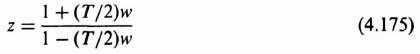
In order to use the Bode diagram and the simplicity of the logarithmic plots, which are based on the property that the stability boundary is the imaginary axis in the s-plane, we have to transform the z transform into the w-plane, where
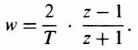

Figure 4.13 Mapping of the primary strip in the left half of the s-plane into the z-plane and from the z-plane to the w-plane. (a) Primary strip in the left half of the s-plane. (b) Mapping of the primary strip of the s-plane into the z-plane. (c) Mapping of the unit circle in the z-plane into the w-plane.
Using this transformation, the unit circle of the z-plane is transformed into the imaginary axis of the w-plane. This is illustrated in Figure 4.13c. Therefore, as ω varies from 0 to jωs/2 along the jω axis in the s-plane, w varies from 0 to infinity along the positive jν axis in the w-plane, where the fictitious frequency in the w-plane is defined to be ν where w = jν. The Bode diagram method in the w-plane is presented in detail in Section 4.9.
A. Techniques of z Transformation
The z transformation for various types of time functions will now be considered. These can be found through a direct application of Eq. (4.4) or (4.30). Attention will be focused on those types of functions which are common to feedback control systems. Several examples will be used to illustrate the techniques prior to tabulating several useful transform pairs:
1. The z Transform of a Unit Step

where r(nT) = 1, for n = 0, 1, 2,…,
This series is convergent for [z] > 1, and yields

2. The z Transform of a Unit Ramp
where r(nT) = 0, T, 2T, 3T, 4T, etc., for n = 0, 1, 2,…,
This series is convergent for [z] > T, and yields
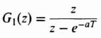
3. The z Transform of an Exponential Decay
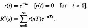
where r(nT) = e−anT, for n = 0, 1, 2,…,
This series is convergent for [z] > e−aT, and yields
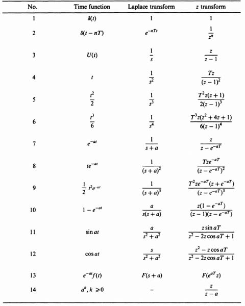
Once the z transform for any function is obtained and tabulated, it is not necessary that it be derived again. Tabulations of the foregoing results, and other transform pairs useful to the control engineer, appear in Table 4.1.
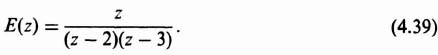
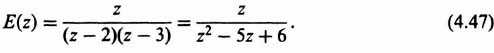
Because it is necessary for the control engineer to obtain the z transform for all of the elements of a feedback control system when analyzing a sampled-data system, it is a useful exercise to obtain the z transform for a typical transfer function that the process may have. Attention will be focused on the technique of application for the z transform of a third-order process whose transfer function is given by

By means of partial fraction expansion, this transfer function can be expressed as
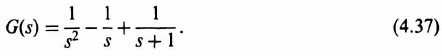
The z transform can be obtained, by inspection, from Table 4.1:

Table 4.1. Table of z Transform
B. Obtaining the Inverse z Transformation
In general, there are four methods for obtaining the inverse z transform. These are by means of partial fraction expansion, power-series expansion, the inversion integral, and the digital computer computational method. Each of these techniques is outlined as follows:
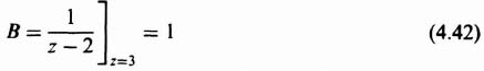
1. Partial Fraction Expansion. The z transform is factored into its components so that each term of the expansion can be obtained, by inspection, from Table 4.1 as was illustrated in the preceding example. The technique for partial fraction expansion is also applicable to the z transform. For example, consider the following transfer function:
The partial fraction expansion is obtained as follows:
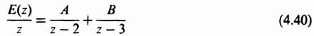
where

Therefore,
From Table 4.1, the inverse z transformation of E(z) is given by:
This can also be written in the following form:
2. Power-Series Expansion. The z transform can be expanded into an inverse power series in z by expanding Eq. (4.30). The result is
The coefficient of z−n, e(nT), is the value of the variable at the nth sensing instant, and the coefficients can be used directly to find the time function at the sampling instants. For example, let us reconsider Eq. (4.39) and obtain its inverse z transformation using the power series expansion as follows:
Dividing denominator into numerator, we obtain the following:
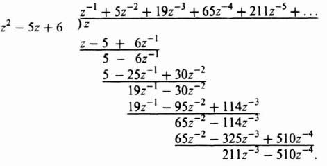
Therefore,
From Table 4.1, the inverse z transform of E(z) is given by:
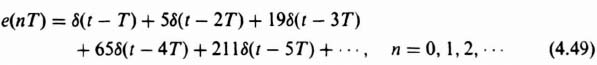
This can also be written in the following form:

Let us check our results from Eq. (4.50) with that of Eq. (4.45). For example, let us check the value of Eq. (4.45) at k = 3:
![]()
This result agrees with the value at k = 3 in Eq. (4.50). Let us also check the value of Eq. (4.45) at k = 5:
![]()
This result also agrees with the value at k = 5 in Eq. (4.50). We, therefore, conclude that Eq. (4.50) is the series form of the closed-form solution obtained in Eq. (4.45).
3. Computation using a Digital Computer. A digital computer can be a very powerful tool for obtaining the inverse z transform. The approach involves converting the z transform into a difference equation that can then be solved using a digital computer. For example, let us reconsider the transfer function which was evaluated in Eqs. (4.39) and (4.47):

We wish to obtain the impulsive response of such a system. From Table 4.1, we know that the z transform of a unit impulse is 1. Therefore, with R(z) representing a unit impulse whose z transform is 1, we obtain

from which
Using Table 4.1, the difference equation corresponding to this equation is
where the unit impulse implies that r(0) = 1 and r(n) = 0 for all other n. The solution to this difference equation depends on the initial conditions e(0) and e(1). The value of e(0) can be obtained by substituting n = −2 into the difference equation for e(n + 2); the result is e(0) = 0. Similarly, the value of e(1) can be obtained by substituting n = −1 into the difference equation; the result is e(1) = 1.
The problem of solving for e(n) reduces to solving the difference equation subject to the following initial conditions: e(0) = 0; e(1) = 1; r(0) = 1; r(n) = 0 for all other n. A program, written in Basic, for solving the difference equation subject to the initial conditions is shown in Table 4.2. The output obtained from the digital computer for this problem is shown in Table 4.3. The results were then checked with the solutions for this problem that were obtained using the previous inversion integral method. The results were identical. The program shown in Table 4.2 is a very useful program for solving difference equations, and can be modified for other problems by changing the initial conditions on line 100 (which is read in on line 10) and the elements of the difference equation on line 30.
C. Example of Simple, Open-Loop Sampled-Data System
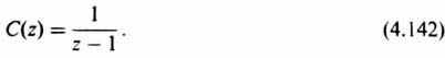
Let us now extend our development of z-transform theory to the case of a simple, open-loop, sampled-data system illustrated in Figure 4.14a. The input function r(t) is a unit step. The sampling rate T is 1 sec. The output c*(t) is to be assumed sampled by an imaginary sampler synchronized with the real one. Let us apply the techniques of z-transform theory in order to obtain R(z), C(z), and c*(t).
Table 4.2. Computer Program (in Basic) for Solving the Difference Equation e(n + 2) − 5e(n + 1) + 6e(n) = r(n + 1) having the Following Initial Conditions: e(0) = 0; e(1) = 1; r(0) = 1; r(n) = 0 for all other n
| 10 | READ E2, E1, R1, R0 |
| 20 | For N = 0 TO 14 |
| 30 | E0 = R1 + 5*E1 – 6*E2 |
| 40 | PRINT N,E0 |
| 50 | E2 = E1 |
| 60 | E1 = E0 |
| 70 | R1 = R0 |
| 80 | R0 = 0 |
| 90 | NEXT N |
| 100 | DATA 0, 0, 0, 1 |
Table 4.3. Output of Program in Table 4.2

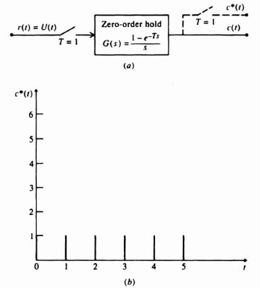
Figure 4.14 Analysis of a simple, open-loop, sampled-data system.
![]()
R(z) can be obtained from Table 4.1 (and our previous derivation):
2. Computation of C(z). The z transform of the output of a network is equal to the z transform of the input multiplied by the z-transfer function of the network. Therefore, for Figure 4.14a,
The z transform of the zero-order hold, shown in Figure 4.14a, is given by
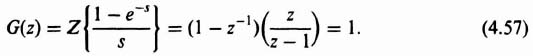
where Z indicates the z transform corresponding to the bracketed Laplace-transform term. Substituting Eqs. (4.55) and (4.57) into Eq. (4.56) we obtain the expression
Dividing denominator into numerator, we obtain the series given by
3. Computation of c*(t). The value of c*(t) can be obtained from the power-series expansion given by Eq. (4.5). Utilizing Table 4.1, we obtain
![]()
The output c*(t) is illustrated in Figure 4.14b.
D. Other Properties
There are certain other properties of the z transform that are worthy of mention. The initial- and final-value theorems relate the initial and final values of a time function to its associated z transform. They are given by
Applying the initial- and final-value theorems as given by Eqs. (4.60) and (4.61), respectively, to the problem illustrated in Figure 4.14, we obtain the following. (a) Initial value:
where C(z) is given by Eq. (4.59).
This result agrees with the sketch of Figure 4.14b. (b) Final value:
where C(z) is given by Eq. (4.58).
This result also agrees with the sketch of Figure 4.14b.
E. Advanced z-Transform Method
A very powerful tool that can be used to evaluate the response between sampling instants is the advanced z-transform method [7]. This technique essentially consists of modifying the ordinary z transform by inserting a fictitious time delay into the sampled-data control system. The resultant transform describes pulse sequences that are delayed from the time functions by nonintegral multiples of the sampling frequency. By varying the amount of delay, the information contained in the continuous signal between sampling instants can be studied.
The advanced z transform can best be understood by referring to the time function in Figure 4.15, which is delayed by αT sec:
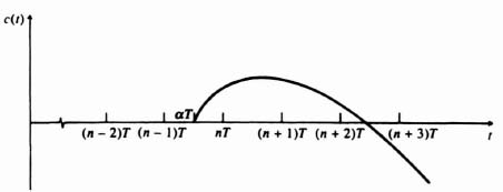
Figure 4.15 Time function delayed by αT sec.
If α is an integer, the result is redundant, because the z transform of the resulting function is merely z−αC(z). The value of n is chosen as the next highest integer after α, making it an advance. The difference of nT and αT is defined as Δ, where
or
Δ is assumed to be a positive number between zero and unity.
Assuming that C(s) is the Laplace transform of c(t), then the Laplace transform of the delayed function, C(s, α), is given by
Substituting Eq. (4.67) into Eq. (4.68), the following expression can be obtained:
The advanced z transform corresponding to Eq. (4.69) is given by
where Z indicates the z transform corresponding to the bracketed Laplace-transform term.
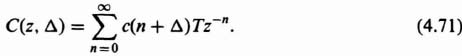
From the definition of the z transform, the advanced z transform can be expressed in the following general form:
As an example of the advanced z-transform derivation for a time function, the case of an exponential decay, eαT, that is advanced by 0.2T sec will be considered. For this problem,
Utilizing Eq. (4.72), the advanced z transform corresponding to this expression is given by
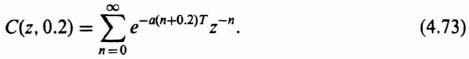
This can be simplified to

The infinite geometric progression corresponding to Eq. (4.74) can be expressed in closed form by

Utilizing this approach, a table of advanced z transforms for several functions can be derived. Table 9.4 lists the advanced z transforms for some commonly found functions.
The inverse of the advanced z transform enables the control-system engineer to evaluate the system's response between samples directly. For example, let us consider a system where G(s) = 1/(s + 1), and let us further assume that the input is a unit step. From Table 4.4, the corresponding advanced z transform corresponding to the input R(s) is given by

and that for the control element G(s) is given by
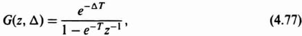
Table 4.4. Table of Advanced z Transforms

The advanced z transform of the output, C(z, Δ), is given by
or

By keeping Δ as a constant parameter, the inversion of Eq. (4.79) results in the following expression:
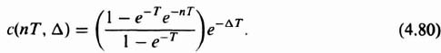
Therefore, if the response following the nth sampling interval is desired, the value of n is substituted into this expression and Δ is allowed to vary from zero to unity. As would be expected, the continuous function between any sampling interval is an exponential decaying term whose initial value is that in the parentheses.
4.5. z-TRANSFORM BLOCK-DIAGRAM ALGEBRA
The procedure for determining the z-transfer function of sampled-data systems is complicated by the absence of samplers between elements, and it is impossible to obtain a direct analogy with the rules governing the reduction of continuous systems.
Let us initially consider two elements in cascade separated by a sampler as is illustrated in Figure 4.16. The z transform of the output from the second sampler, C1(z), is
The z transform of the output from the last sampler, in terms of C1(z), is
Substituting Eq. (4.82) into Eq. (4.81), we obtain
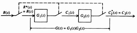
Figure 4.16 Cascaded elements separated by a synchronous sampler.
and conclude that the z transforms of cascaded elements separated by samplers equal the product of the z transforms of the individual cascaded elements.
Let us next consider the configuration where a sampler does not separate cascaded elements, as is illustrated in Figure 4.17. Notice that the second element is driven by the value c1(t) at the sampling instants, and also between the sampling instants. For this case, the z transform of the output is given by
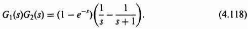
where G1G2(z) represents the z transform of the cascaded combination corresponding to the transfer function G1(s)G2(s). It is very important to emphasize here that G1G2(z) is very different from G1(z)G2(z). A very simple example will illustrate the difference implied by Eqs. (4.83) and (4.84). Consider that

and

For the system illustrated in Figure 4.16,
![]()
From Table 4.1, the individual z transforms are
and

Substituting these z transforms into Eq. (4.83), we obtain

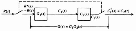
Figure 4.17 Cascaded continuous elements not separated by a sampler.
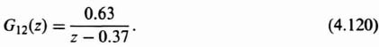
For the connection illustrated in Figure 4.17,
The term G1G2(z) corresponds to the z transform of G1(s)G2(s)a, where
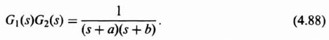
By means of partial fraction expansion, Eq. (4.88) can be written as

The z transform of Eq. (4.89), G1G2(z), can be obtained by inspection from Table 4.1 as follows:
Observe the great difference between Eqs. (4.90) and (4.86).
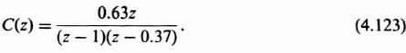
Let us next determine the z transform of the output for several versions of sampled-data feedback control systems. We shall specifically derive C(z) for the systems illustrated in Figures 4.18a, b, c, and d.
A. Sampler in Error Channel (Figure 4.18a)
The closed-loop transfer function can be derived in the following manner:
Because the sampler is a linear device and superposition is valid, we can write
Solving Eq. (4.92) for E*(s), we obtain
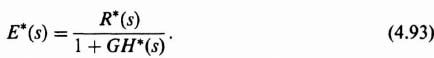
Because
we obtain the value of C(s) as
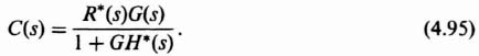
Taking the z transform of Eq. (4.95), the following results:
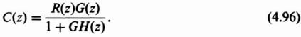
Equation (4.96) gives the value of the output at the sampling instants for the configuration of Figure 4.18a.

Figure 4.18 Various versions of sampled-data control systems. (a) Sampler in error channel. (b) Sampler in feedback loop. (c) Synchronous samplers in forward loop. (d) Synchronous samplers and cascaded elements in forward loop.
B. Sampler in Feedback Loop (Figure 4.18b)
The z transfer function of the output can be derived in the following manner:
and
Substituting Eq. (4.97) into Eq. (4.98), we obtain
Taking the z transform of Eq. (4.99) the following results:
Simplifying, we obtain

Equation (4.101) gives the value of the output at the sampling instants for the configuration of Figure 4.18b.
C. Synchronous Samplers in Forward Loop (Figure 4.18c)
The z transfer function of the output can be derived in the following manner:
Because the sampler is a linear device, and superposition is valid, we can write
Solving Eq. (4.103) for E*(s), we obtain
In addition, because
we obtain the relation between C*(s) and R*(s) as
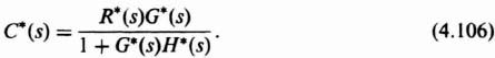
Taking the z transform of Eq. (4.106), the following results:
Equation (4.107) gives the value of the output at the sampling instants for the configuration of Figure 4.18c.
D. Synchronous Samplers and Cascaded Elements in Forward Loop (Figure 4.18d)
The z-transfer function of the output can be derived in the following manner:
Because the sampler is a linear device and superposition is valid, we can write
Solving Eq. (4.109) for E*(s), we obtain

In addition, because
we obtain the value of C(s) as

Taking the z transform of Eq. (4.112) the following results:
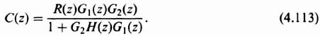
Equation (4.113) gives the value of the output at the sampling instants for the configuration of Figure 4.18d.
It is important to recognize that the concepts of signal-flow graphs developed in Sections 2.14–2.16‡ for continuous systems can be extended to discrete systems with some modifications. In particular, Mason's theorem stated in Eq. (2.135)‡ can be used for discrete systems with some modifications, based on the results shown in this section. The following rules should be used in adapting Mason's theorem for discrete systems:
- If the input R(s) is not separated from the first element in the forward part of the loop [e.g., G(s)] by a sampler, then the z transform of the input and the first element cannot be separated, and a term RG(z) will result. Therefore, a transfer function of output/input cannot be obtained (e.g., Figure 4.18b, Eq. [4.101]).
- For an element in the forward or feedback part of the loop to occur as a stand-alone transfer function in terms of z [e.g., G(z)], then that element must be separated from all other elements by a sampler at its input and output. For example, G(s) in Figure 4.18c and G1(s) in Figure 4.18d satisfied this requirement.
- If an element in the forward or feedback part of the loop is not separated from an adjacent element (or the input) by a sampler, then it is necessary to take the z transform of the combined transfer function of the two elements (or the element and the input). We saw examples of this in Figures 4.18a and b [G(s) and H(s)], G2(s) and H(s) in Figure 4.18d, and R(s) and G(s) in Figure 4.18b of this section.
It is left as an exercise to the reader to check the results of the four examples illustrated in this section with Mason's theorem using the three modifications stated.
4.6. CHARACTERISTIC RESPONSE OF A SAMPLER AND ZERO-ORDER HOLD COMBINATION
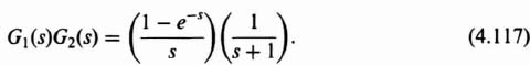
The tools developed so far have made it possible for us to determine the characteristic response of the sampler and zero-order hold combination illustrated in Figure 4.19 to various types of inputs. We shall apply the z-transform theory in order to determine its response to inputs of a unit step and ramp. We shall assume that the sampling time T is 1 sec and that the transfer function G2(s) is given by
The z-transfer function of this open-loop system, corresponding to the transfer function G1(s)G2(s), is denoted by G12(z). The zero-order hold transfer function G1(s) was derived previously, and is given by Eq. (4.19) as

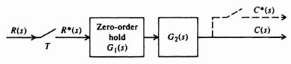
Figure 4.19 Sampler, zero-order hold and process G2(s) in cascade.
Because T = 1, Eq. (4.115) reduces to
Therefore,
By means of a partial fraction expansion, Eq. (4.117) can be written as
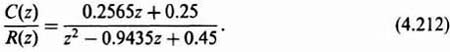
The z transform of Eq. (4.118) can be obtained from Table 4.1 by inspection. Its value is

This relation can be simplified to the following:
For a given input, whose z transform is R(z), the z transform of the output can be expressed as
The characteristic response to inputs of a unit step and ramp are computed as follows:
A. Unit Step Input
![]()
From Table 4.1,
Substituting Eqs. (4.120) and (4.122) into Eq. (4.121), we obtain

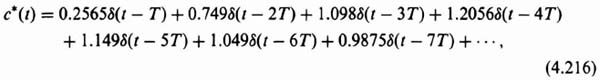
The inverse z transform can be obtained by expanding Eq. (4.124) into a power-series expansion in z and then taking the inverse z transform by utilizing Table 4.1. The expression for a power-series expansion in z is given by
By utilizing Table 4.1 the inverse z transform can be expressed as

The result is sketched in Figure 4.20.
B. Unit Ramp Input
![]()
From Table 4.1.

Because T = 1, Eq. (4.127) reduces to

Figure 4.20 Output response of the circuit shown in Figure 4.19 to a unit step input.
Substituting Eqs. (4.120) and (4.128) into Eq. (4.121), we obtain

This can also be expressed as
The inverse z transform can be obtained by expanding Eq. (4.130) into a power-series expansion in z and then taking the inverse z transform by utilizing Table 4.1. The expression for a power-series expansion in z is given by
By utilizing Table 4.1 the inverse z transform can be expressed as

The result is sketched in Figure 4.21.
From the results illustrated in Figures 4.20 and 4.21, we conclude that the zero-order hold can respond with zero steady-state error to a unit step input but not to higher-order inputs such as a ramp. This is to be expected from our previous discussion of data extrapolators in Section 4.3.
4.7. STABILITYANALYSIS USING THE NYQUIST DIAGRAM
The Nyquist stability criterion for continuous systems was described in Section 1.7. This section will show how to extend the Nyquist diagram for continuous systems to discrete systems. For the discrete case, we will show that the ideas are identical to the continuous case with the exception that the contours enclosing the unstable region of the z-plane are outside the unit circle as shown in Figure 4.22. This stability concept

Figure 4.21 Output response of the circuit shown in Figure 4.19 to a unit-ramp input.

Figure 4.22 Contour used to enclose poles in the z-plane outside the unit circle.
was introduced in Section 4.4 (see Figures 4.12 and 4.13). The corresponding Nyquist stability criterion of Eq. (6.63)‡ for continuous systems is modified for discrete systems to
where N is the number of clockwise encirclements of the −1 + j0 point for the GH(z) or G(z)H(z) contour for z taking values shown on Figure 4.22, P is the number of unstable poles of GH(z) or G(z)H(z), and Z is the number of unstable roots of the characteristic equation. Phase and gain margins defined for continuous systems in Eqs. (6.67)‡ and (6.69)‡ and Section 1.7 for the G(s)H(s) plane, respectively, are exactly the same for discrete systems in the GH(z) or the G(z)H(z) plane.
It is interesting to observe from Figure 4.18 that the system transfer functions for the various versions of sampled-data control systems generally can be written as

where N(z) = z transform of the open loop.
For the configuration of Figure 4.18a, where the sampler is in the error channel, M(z) = G(z) and N(z) corresponds to the z transform of the continuous Laplace transfer function G(s)H(s). Therefore,

For purposes of analyzing stability using the Nyquist diagram, we shall study the form given in Eq. (4.135). However, it should be emphasized that the technique used is applicable to any configuration of sampled-data control system.
The characteristic equation of a sampled-data control system, given by the denominator of Eq. (4.134) is
For the case of the sampled-data control system having a sampler in the error channel, the characteristic equation is given by
In accordance with the discussion of stability in Section 4.4, a closed contour having a radius of unity is examined in the z-plane. The area enclosed by the contour covers the entire region outside the unit circle. This is illustrated in Figure 4.22. The map of this contour, in the 1 + GH(z) plane, indicates by its enclosure of the origin the difference between the zeros and poles of this function in accordance with Cauchy's theorem. Specifically, the number of times the map of this contour encloses the origin equals the difference between the number of poles and zeros. This is the same as for the Nyquist diagrams applied to continuous systems which were discussed in Section 1.7.
It is important to realize that if GH(z) is a stable function, then 1 + GH(z) will also be stable. In sampled-data systems, it is convenient to shift the imaginary axis to the point (−1, 0) just as was done in the case of continuous systems. When the axis is shifted in this manner, it is necessary to consider only GH(z) and study the enclosure of the point (−1, 0) rather than the origin.
Practical sampled-data control systems usually contain one or more integrations among the continuous elements. From Table 4.1, it can be seen that the z transform of an integration results in a pole in the z-plane at the point (1, 0). This pole would cause a discontinuity if the contour being mapped were exactly the one shown in Figure 4.22. Therefore, it is necessary to generate a small semicircular detour around the pole at z = 1 in order to establish a connection between the segments of the contour. This is illustrated in Figure 4.23. The detour is conventionally oriented in order to include the pole inside the unit circle. Due to the fact that practical values of GH(z) vanish for infinite values of z, and because the segment of the contour along the real axis cancels itself in the limit, only the unit circle and its detours are usually mapped. This is illustrated in Figure 4.24.
We next apply the Nyquist stability criterion to the configuration illustrated in Figure 4.18a for two different values of the process, G2(s).
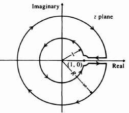
Figure 4.23 Contour used to enclose poles in the z-plane outside the unit circle when integrations are present.

Figure 4.24 Reduced contour for mapping practical values of GH(z).
A. System of Figure 4.25
The sampled-data control system illustrated in Figure 4.25 contains a sampler in the error channel followed by a zero-order circuit and a pure integrator. We wish to determine whether the system is stable when K = 1, the maximum value of K before the system becomes unstable, and the system's response to a unit-step input. The sampling time will be assumed to be 1 sec.
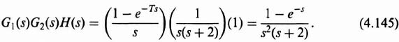
1. System Stability (K = 1). The system stability can be determined by examining the locus of GH(z) in the GH(z) plane. The Laplace transfer function corresponding to G1(s)G2(s)H(s) is
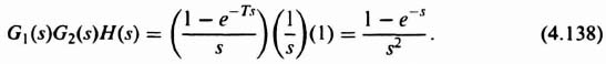
From Table 4.1, the z-transfer function GH(z) corresponding to Eq. (4.138) is
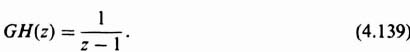
The locus of GH(z) is shown in Figure 4.26. Because the locus does not enclose the −1 + j0 point, the Nyquist criterion is satisfied and the system is stable.
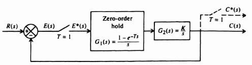
Figure 4.25 Sampled-data control system containing a zero-order hold and an integrator.

Figure 4.26 Locus in GH(z) plane of system shown in Figure 4.25.
2. Maximum Value of Gain. The maximum value of gain K that is theoretically possible before the system becomes unstable can also be found from the locus of GH(z) in the GH(z) plane. This is illustrated in Figure 4.26. It can easily be seen that if the gain were doubled, the locus would pass through the −1, 0 point. Therefore, the maximum value of K, before the system becomes unstable, is 2. Note that the gain margin is 6 dB.
3. System Response to a Unit Step. From Figure 4.18a, the z transform of the system output equals

From Table 4.1, the z transform of a unit step equals
Substituting Eqs. (4.139) and (4.141) into Eq. (4.140), we obtain
By expanding Eq. (4.142) into a power series in z, and then taking the inverse z transform, the output response can be plotted. The result is
and is plotted in Figure 4.27. Therefore, the system behaves as a critically damped system in its response to a unit step input.
B. System of Figure 4.28
Let us next consider the sampled-data control system illustrated in Figure 4.28. It contains a sampler in the error channel followed by a zero-order hold circuit and a second-order process. For this configuration, we wish to determine whether the system is stable when K = 1, the maximum value of K before the system becomes unstable, and the system's response to a unit step input. The sampling rate will be assumed to be 1 sec.
1. System Stability (K = 1). The solution to this problem is similar to the previous problem. The Laplace transformation function G1(s)G2(s)H(s) equals
By utilizing a partial fraction expansion of the denominator and Table 4.1, the z-transfer function GH(z) corresponding to Eq. (4.145) can be obtained. Its value is
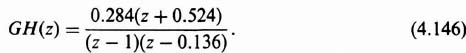
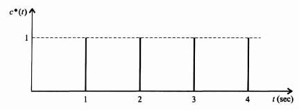
Figure 4.27 Output response of the system shown in Figure 4.25 to a unit step input.
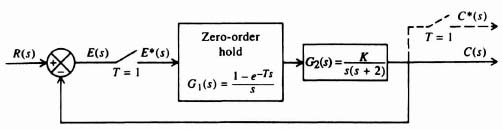
Figure 4.28 Sampled-data control system containing a zero-order hold and a second-order process.
The locus of GH(z) is shown in Figure 4.29. Because the locus does not enclose the −1 + j0 point, the Nyquist criterion is satisfied and the system is stable.
2. Maximum Value of Gain. The maximum value of gain K that is theoretically possible before the system becomes unstable can be found from the locus of GH(z) in the GH(z) plane. This is illustrated in Figure 4.29. It can easily be seen that if the gain were increased by a factor of 1/0.170 = 5.88, the locus would pass through the −1, 0 point. Therefore, the maximum value of K, before the system becomes unstable, is 5.88. Note that the gain margin is 15.39 dB.
3. System Response to a Unit Step. The system response to a unit step can easily be determined by substituting Eqs. (4.141) and (4.146) into Eq. (4.140). The result
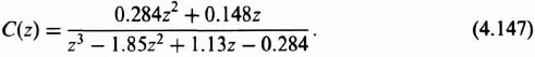
By expanding Eq. (4.147) into a power series in z and then taking the inverse z transform, the output response can be plotted. The result is


Figure 4.29 Locus in the GH(z) plane.
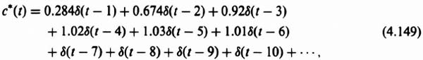
and is plotted in Figure 4.30. Therefore, the system has an overshoot of only 3% in its response to the unit step input, and has zero steady-state error.
4.8. STABILITY DETERMINATION USING MATHEMATICAL TESTS
Stability of sampled-data control systems can also be determined through the application of several mathematical tests. This section will present the modified Routh–Hurwitz criterion, the Schur–Cohn stability criterion, and Jury's stability criterion.
A. The Modified Routh–Hurwitz Criterion
Stability of sampled-data control systems cannot be determined by means of a direct application of the Routh–Hurwitz criterion. However, it is possible to apply a transformation to the characteristic equation z that will transform the region outside the unit circle in the z-plane to the right half of an auxiliary plane, and the region inside the unit circle to the left half of this plane. This transformation, known as the bilinear transformation, has been applied to discrete control systems [3–5, 8]. The auxiliary plane, denoted as the w-plane (see Figure 4.13), is defined by the following relationship:
or

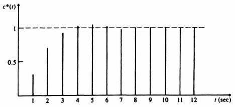
Figure 4.30 Output response of the system shown in Figure 4.28 to a unit step input.
If the Routh–Hurwitz critereon is applied to the characteristic equation, that is, subjected to the transformation of Eq. (4.150), conditions can be found that cause the roots of the transformed equation to lie in the left half of the w-plane. Therefore, it is possible to determine if the roots of the characteristic equation lie within the unit circle of the z-plane using this transformation. The procedure is illustrated next for the system having the form shown in Figure 4.18a.
As an example, let us consider the following closed-loop system transfer function:

whose characteristic equation is given by
Using the bilinear transformation of Eq. (4.150) on Eq. (4.153), we obtain
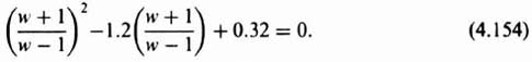
Simplifying this expression, we obtain
Application of the Routh–Hurwitz criterion to Eq. (4.155) yields the following array (see Section 6.3‡):
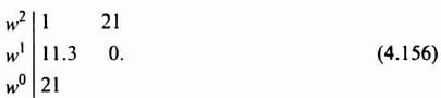
Because there are no sign inversions in the left column of the resulting array, this system has no poles in the right half of the w-plane, or outside the unit circle of the z-plane, and is stable. As a check, we can factor the second-order characteristic equation of Eq. (4.153) and determine that the closed-loop roots in the z-plane are located within the unit circle at z =0.4 and 0.8.
B. The Schur–Cohn Stability Criterion
Although the modified Routh–Hurwitz criterion is simple to apply in principle, it is quite laborious for higher-order systems. For these cases, the Schur–Cohn [9, 10] stability criterion and Jury's [2, 10, 11] stability criterion are quite useful.
The Schur–Cohn stability criterion states that a sampled data control system is stable if the sequence of Schur–Cohn determinants, 1, Δ1, Δ2,…, Δj,…, Δn, has n variations in sign. Another way of stating this particular stability criterion is that
in order for the system to be stable.
Assuming that the characteristic equation of the linear sampled data control system is given by
Then the jth Schur–Cohn determinant is defined as
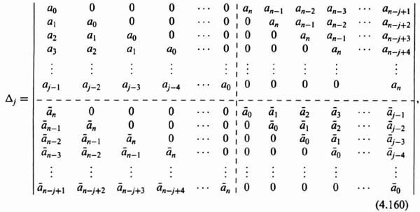
where j = 1, 2, 3, 4,…, n and ![]() is the conjugate of aj. Assuming that all of the coefficients of the characteristic equation are real, then the determinant Δj is symmetrical with respect to its principal diagonal.
is the conjugate of aj. Assuming that all of the coefficients of the characteristic equation are real, then the determinant Δj is symmetrical with respect to its principal diagonal.
It is interesting to observe that if the conditions of the Schur–Cohn stability criterion are not satisfied, then we merely know that the characteristic equation has at least one root which lies outside the unit circle in the z-plane. Unlike the Routh–Hurwitz criterion, this criterion does not indicate the number of roots which lie on or outside the unit circle.
The Schur–Cohn stability criterion will next be applied to a simple system of the form shown in Figure 4.18a, where

whose characteristic equation is given by
The Schur–Cohn determinant Δ1 of this equation is given by

Therefore, the sequence of Schur–Cohn determinants for this simple case is 1, 0.
Because Δ1 is not less than zero, this system is unstable based on the Schur–Cohn stability criterion. As a check, we can factor the second-order characteristic equation of Eq. (4.162) and determine that the closed-loop roots in the z-plane are located at z = 0.5 and 2. The root at 2 is outside the unit circle, and verifies that this system is unstable.
C. Jury's Stability Criterion
The stability criterion devised by Jury [2, 10, 11] is much simpler to apply than the Schur–Cohn stability criterion. The first step in Jury's stability criterion is the formation of the following table from the characteristic equation:
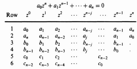
Note that the elements of even rows consist of the coefficients of odd rows written in reverse order. The values in the third row are formed from the second-order determinants using the first column of the first two rows with each of the other columns from these rows, and starting from the right and dividing by the coefficient a0. Therefore, the terms b0, b1, and bj, are given by

The fourth row is obtained by reversing the elements in the third row, and the process is repeated. The elements in the fifth row are given by
Jury's stability criterion requires that all the terms of the odd rows in the left column be positive for the system to be stable (has all roots inside the unit circle of the z plane). This is a sufficient and necessary condition for all the roots of the characteristic equation to lie inside the un it circle in the z-plane.
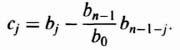
As an example for applying Jury's stability criterion, let us consider the following characteristic equation:
The resulting Jury array is given by
Because the terms in the left column of the odd rows are positive, the system having the characteristic equation of Eq. (4.164) is stable. As a check, we can determine that the roots of this third-order characteristic equation are at −0.4973 and 0.7987 ± 0.408j. Because all of the roots are inside the unit circle in the z-plane, the system is stable.
The Routh–Hurwitz criterion mathematical test does not show how to improve design. It merely tells the control-system engineer whether the system is stable or unstable. The same is true for the three mathematical tests presented in this section for discrete systems. The modified Routh–Hurwitz criterion, the Schur–Cohn stability criterion, and Jury's stability criterion tell the control-system engineer whether a discrete control system is stable or not, but give no information on the location of the roots in the z-plane, For example, if any of these three mathematical tests indicate that the system is stable, we do not know how close the roots are to the unit circle in the z-plane. If the mathematical tests indicate that the system is unstable, we do not know how distant the roots are from the unit circle in the z-plane. The main attributes of these mathematical tests are to serve as a check on other design methods and to give a quick answer to the question of stability.
4.9. STABILITY ANALYSIS AND DESIGN USING THE BODE DIAGRAM
The usefulness of the Bode diagram, as presented in Chapter 1 for continuous systems, is lost for discrete systems in the z-plane due to the relationship between z and s:
However, we can extend the usefulness of the Bode diagram for continuous systems to discrete systems by means of the bilinear transformation, which was presented in Section 4.8, Eq. (4.151),

and used for the modified Routh–Hurwitz criterion. Before we can use this transformation constructively for the Bode diagram, a modification must be made to Eq. (4.166), because this definition of the bilinear transformation lacks the desirable property that as the sampling time T approaches zero, we want w to approach s. This limitation can be overcome by defining a modified bilinear transformation [2–5], where

For example, with the definition of Eq. (4.167) the relationship between wand s, as T approaches zero, is given by

Therefore, the definition of Eq. (4.167) has the desirable property that w approaches s as T approaches zero. In this section on the extension of the Bode diagram to discrete systems, we will use the modified bilinear transformation defined by Eq. (4.167).
By means of the z transformation and the w transformation, the primary strip of the left half of the s-plane shown in Figure 4.13 is mapped inside of the z-plane's unit circle and then mapped into the left half of the w-plane. Therefore, as s varies from 0 to jws/2 along the jω axis in the s-plane, w varies from zero to infinity along the positive jν axis in the s-plane. We designate the fictitious frequency on the w-plane to be ν, where
After we make the transformation of G(z) to G(w), we can then treat G(w) as a conventional transfer function in w. By replacing w by jν, we can then use the conventional Bode diagram for analyzing the transfer function in terms of w. Therefore, all of the straight-line approximation magnitude plots we used to draw the Bode diagram for continuous systems in Chapter 1 and Chapter 2 are adaptable to discrete systems in the w-plane.
We will illustrate the approach through an example. Let us consider the system shown in Figure 4.31, which contains a zero-order hold and a process which is represented by a double integration. The resulting open-loop transfer function is given by
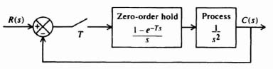
Figure 4.31 A sampled-data control system containing a zero-order hold and a process which is a double integration.
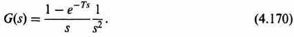
Its z transform is given by
From Table 4.1, we find that the z transform of 1/s3 is given by

Substituting Eq. (4.172) into Eq. (4.171), we obtain the following z transform:
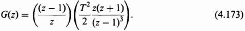
Simplification of Eq. (4.173) results in the following:
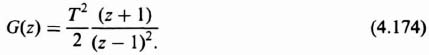
To find the w transform of Eq. (4.174) we solve Eq. (4.167) for z in terms of w
and substitute it into Eq. (4.174)
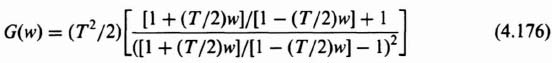
Simplifying Eq. (4.176), we obtain

For this example, let us assume that the sampling time T is 0.26 sec. Therefore, Eq. (4.177) reduces to
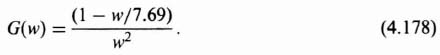
In terms of the frequency ν, where w = jν, Eq. (4.178) can be written as

There are several interesting things to observe In comparing Eq. (4.178) [or (4.179)] with the process to be controlled:
The gains of both transfer functions are the same and they will be in all cases. In addition, the denominators are identical in this case, although this may not be true in all cases. However, as T approaches zero, the denominators will be identical in all cases. The zero term in the numerator in the right half-plane is due to the sample and zero-order hold, and is a function of the sampling rate T. It is important to recognize that although this zero term provides a negative phase contribution (similar to a pole's effect) because it is in the right half-plane, it does contribute a + 20 dB/decade slope (at frequencies greater than its break frequency) to the magnitude plot.
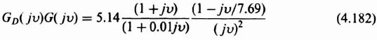
The resulting Bode diagram for Eq. (4.179) is shown in Figures 4.32a and b. It has a gain crossover frequency of 1.017 rad/sec and is unstable with a phase margin of −7.536 degrees. To stabilize this system, we add a phase-lead network GD(w), as shown in Figure 4.33. The design specifications for this system are a gain crossover frequency of 7 rad/sec, a phase margin of approximately 35 degrees, and a gain margin of approximately 3 dB. The design procedure is to add a zero at 1 rad/sec prior to the crossover frequency of 7 rad/sec, because the initial slope of the Bode diagram in Figure 4.31a is −40 dB decade. (Recall Bode's first theorem in Section 2.6). The pole due to the phase-lead network is placed at a frequency much greater than the crossover of 7 rad/sec, Analysis of Figure 4.32a, indicates that the gain is −31.18 dB at the desired crossover frequency of 7 rad/sec (see Figure 4.32a). Therefore, the gain of the system must be increased by 31.18 dB to achieve a crossover frequency of the compensated system at 7 rad/sec. Through trial and error, it was found that by placing the pole of the phase-lead network at 100 rad/sec, the resulting phase margin is 35.33 degrees, and the gain margin is 3.399 dB (phase crossover frequency occurs at 25.72 rad/sec). These are very close to the design specifications and are acceptable. Of the 31.18 dB gain increase, the phase-lead network addition provides + 17 dB at 7 rad/sec. Therefore, the gain has to be increased by 14.18 dB, or 5.14. The resulting attenuation of 0.01 due to the phase-lead network can be made up for by increasing the system's amplitude gain by 100.
The resulting transfer function of the phase-lead network is given by

Figure 4.32 Bode diagram for system shown in Figure 4.31.

Figure 4.33 A phase-lead network added to stabilize the system of Figure 4.31.
The resulting transfer function of the compensated system is given by
and the Bode diagram is shown in Figures 4.34a and b. Figures 4.32 and 4.34 were obtained using MATLAB and are contained in the M-files that are part of my Advanced Modern Control System Theory and Design (AMCSTD) Toolbox which can be retrieved free from The MathWorks, Inc. anonymous FTP server at ftp://ftp.mathworks.com/pub/books/advshinners.
In conclusion, we see from this section that the w transform maps the inside of the unit circle in the z-plane into the left-half of the w-plane. The result is that the s-plane and the w-plane are similar over the regions of interest. Therefore, the conventional straight-line approximations to the magnitude curve, and the concepts of phase and gain margins are valid for the Bode diagram for discrete systems when we apply the w transform.
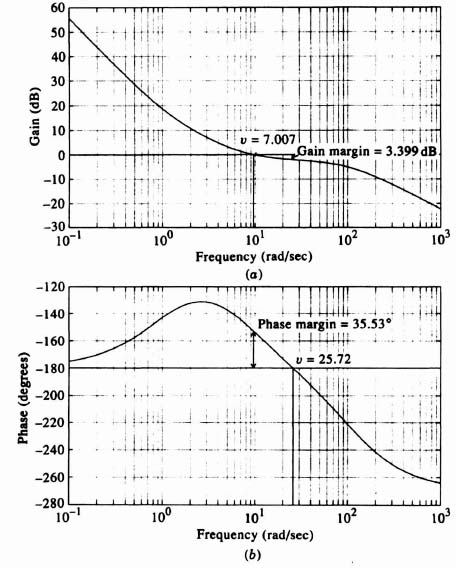
Figure 4.34 Bode diagram of compensated system of Figure 4.33.
4.10. STABIUTY ANALYSIS AND DESIGN USING THEROOT-LOCUS DIAGRAM
We will extend the root-locus concept, developed for continuous systems in Section 1.7 and Section 2.9, to sampled-data systems in this section. Let us consider the sampled-data system of Figure 4.35. From the discussion of z-transform block-diagram algebra in Section 4.5, we recognize that its transfer function is given by the following:

The characteristic equation of this system is given by
Equation (4.184) is analogous to the characteristic equation found in the s-plane root locus. The root locus is a graphical technique for determining the roots of the closed-loop characteristic equation of a system in the s-plane as a function of the static gain. We can extend that definition to sampled-data systems by replacing the words “s-plane” with “z-plane.” Because the characteristic equation of sampled-data systems in the z-plane [Eq. (4.184)] has the same form as characteristic equations of continuous systems in the s-plane, the rules for drawing the root locus shown in Section 6.14‡ for the s-plane are exactly the same for the z-plane. For example, rule 4 for determining portions of the real axis that are part of the root locus, rules 5 and 6 for asymptotic construction, and rule 7 for the points of breakaway and break-in are all the same as those developed for the s-plane.
Although the rules of construction of the root locus in the s- and z-planes are the same, differences lie in interpreting the results. For example, the stable region in the z-plane is in the interior of the unit circle, while the stable region in the s-plane is in the left half-plane. Therefore, the pole locations have different interpretations in the s- and z-planes.
We will illustrate the approach of using the root locus for the analysis and design of a sampled-data system through an example. Let us assume that the sampling period T is held constant and the gain K varies. The root locus may also be plotted as a function of the sampling period T with K held constant. This case is much more complex and beyond the scope of this chapter. This subject is treated in books dedicated to digital control systems such as References 2, 3, and 12.

Figure 4.35 A sampled-data control system with a sampler in the error path.
Let us analyze the negative-feedback sampled-data system illustrated in Figure 4.36. It contains an amplifier having a gain K, a zero-order hold and a process whose transfer function is 1/[s(s + 0.05)]. The z transform of this zero-order hold and process is given by:
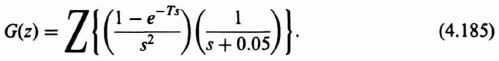
We will assume in this problem that the sampling time T is 1.43 seconds. Therefore, Eq. (4.185) reduces to
We wish to plot the root locus of the open-loop transfer function given by
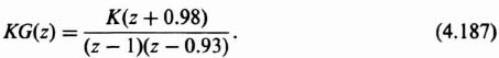
The rules of construction from Section 6.14‡ that are needed to plot the root locus are as follows
Rule 1. This is a second-order system and, therefore, there will be two loci.
Rule 2. The loci start (K = 0) at the two poles located at z = 1 and z = 0.93. One locus terminates (K = ∞) at the finite zero at z = −0.98, and the second locus terminates at a zero at infinity.
Rule 3. Complex portions occur as complex-conjugate pairs.
Rule 4. Portions of the real axis are part of the root locus if an odd number of poles and zeros exist to the right. Therefore, the real axis from −0.98 to −∞ is part of the root locus. In adition, the real axis from 0.93 to 1 has to be part of the root locus.
Rules 5 and 6. The asymptotic rules are not needed in this problem.

Figure 4.36 A sampled-data control system containing an amplifier, zero-order hold and a process whose transfer function is 1/[s(s + 0.05)).
Rule 7. The points of breakaway and break-in are determined from the characteristic equation as follows:

We let the real part of z equal σ′ and solve for K(σ′):

Taking the derivative of K(σ′) with respect to σ′ and setting it equal to zero,
we obtain the following roots:
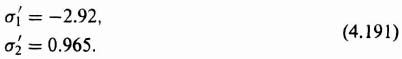
Therefore, there is a breakaway point at 0.965, 0 and a break-in point at −2.92, 0.
Rule 8. The crossing of the imaginary axis and the value of K when it crosses the imaginary axis is obtained using this rule. The characteristic equation is obtained from Eq. (4.188) to be
or
Using the conventional Routh–Hurwitz criterion as presented in Section 6.3‡, we obtain the following array:
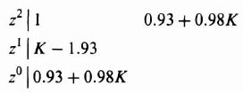
Therefore, from row 2 we find that K = 1.93 when the root locus crosses the imaginary axis. It is important to recognize that this is not Kmax as defined in Section 1.7 for the root locus of continuous systems. It is permissible to use the conventional Routh–Hurwitz criterion here, and not have to use the bilinear transformation presented in Section 4.8, because we are not trying to use rule 8 in this problem to find Kmax. We only want to find K when the root locus crosses the imaginary axis and the value of the imaginary axis at crossing. This point can be found from the real terms of Eq. (4.193) and knowing that K = 1.93 when the root locus crosses the imaginary axis as follows:
Because K = 1.93, we obtain
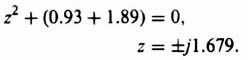
Therefore, the root locus crosses the imaginary axis at ±j1.679.
Rules 9–12. These rules are not needed for this problem.
The resulting root locus, which is shown in Figure 4.37, was obtained using MATLAB (see Section 1.7) and is contained in the M-file that is part of my AMCSTD Toolbox which can be retrieved free from The MathWorks, Inc. anonymous FTP server at ftp://ftp.mathworks.com/pub/books/advshinners. The root-locus diagram illustrated shows that the system is conditionally stable for only very low gains from 0 to 0.07143.
Let us next consider the compensation of this system. How would we proceed to design a compensation network which would make this system stable for a wider range of gain? It is apparent that we must cancel one of the poles at z = 0.93 with a zero placed there. The pole of this compensating network can be placed along the real axis between ±1. A pole at 0.2 was selected, and the resulting network is a phase-lead network. The resulting transfer function of this phase-lead network is given by
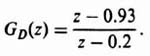
The block diagram of the compensated system is shown in Figure 4.38. Therefore, the open-loop transfer function of the compensated system is given by
which can be reduced to the following:

The root locus of the compensated system, shown in Figure 4.39, was obtained using MATLAB (see Section 1.7) and is also contained in the M-file that is part of the AMCSTD Toolbox. The point of breakaway ![]() and break-in
and break-in ![]() can be obtained using rule 7:
can be obtained using rule 7:
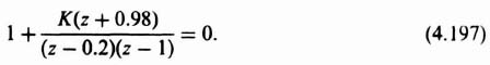

Figure 4.37 Root locus for the system of Figure 4.36.
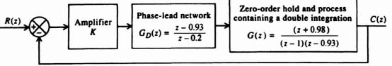
Figure 4.38 System of Figure 4.36 compensated with a phase-lead network, GD(z).

Figure 4.39 Root locus for the system of Figure 4.38.
We let the real part of z equal σ′ and solve for K(σ′):

Taking the derivative of K(σ′) with respect to σ′ and setting it equal to zero,
we obtain the roots 0.55 (breakaway) and −2.50 (break-in). Therefore, the compensated system is conditionally stable as shown in Figure 4.39. The maximum value of K, where the root locus intersects the unit circle, will be obtained using the modified Routh–Hurwitz criterion and the bilinear transformation presented in Section 4.8:
Substituting Eq. (4.200) into the characteristic Eq. (4.197), we obtain the following Routh–Hurwitz array in the w-plane:

Setting the second and third rows of the array equal to zero, we get
![]()
Therefore, the system is stable for 0 < K < 0.8193
What value of K should we select for a desired damping ratio for the compensated system? To answer this question, we note an important difference between finding the damping ratio for a continuous system in the s-plane and a digital control system in the z-plane, We saw in Figure B.3 and Eq. (B.18) that the damping ratio for a second-order system was given in the s-plane by
In the s-plane, the loci for a constant damping ratio ζ, as ωn is varied from zero to infinity, is a straight line, as illustrated in Figure B.3. In the z-plane, the loci for a constant damping ratio ζ, as ωn is varied from zero to infinity, is a logarithmic spiral as illustrated in Figure 4.40. This figure was obtained using MATLAB (see Section 1.7) and is contained in the M-file that is part of the AMCSTD Toolbox which can be retrieved by the reader free from The MathWorks, Inc. anonymous FTP server at ftp://ftp.mathworks.com/pub/books/advshinners.
The reason that the loci for a constant damping ratio ζ in the z-plane is a logarithmic spiral will now be proven. From Figure B.3, the location of the complex-conjugate root in the upper half of the s-plane is given by
Let us transform Eq. (4.202) into the z-plane using z = eTs as follows:
We can rewrite Eq. (4.203)
as and simplify it to
Equation (4.205) is in polar form. Because we are assuming that the damping ratio and the sampling time T are constant, then as ωn increases, the amplitude of z decreases exponentially as the phase angle rotates. Therefore, Eq. (4.205) is the equation of a logarithmic spiral. For example, when ωn = 0, z = 1 ![]() , and when ωn → ∞, z → 0 as illustrated in Figure 4.40.
, and when ωn → ∞, z → 0 as illustrated in Figure 4.40.

Figure 4.40 z plane with constant damping ratio loci.
Let us return to our design problem, and assume that we desire a damping ratio of 0.45. The root locus in Figure 4.39 is redrawn in Figure 4.41 with the constant damping ratio spiral of 0.45 superimposed on the root locus. From the intersection of the root locus and the constant damping ratio loci of 0.45, we see that the root location needed to achieve this damping is at
(The other root is located at z = 0.472 − j0.477.) We can now proceed to find the value of K needed from the characteristic equation with these root locations as follows:


Figure 4.41 Root locus for the system of Figure 4.38 with a loci for a constant damping ratio of 0.45 superimposed.
Solving for K,

Substituting Eq. (4.206) into (4.208), we obtain the following:

Solving for K, we obtain
We wish to check that this value of K will result in a damping ratio of 0.45. The percent overshoot of the system can be determined by solving for C(z) from the following equation:

The inverse z transform will be obtained to find c*(t), from which the maximum percent overshoot (and consequent damping) of the system will be determined. Substituting Eqs. (4.196) and (4.210) into Eq. (4.211), we obtain
To find the percent overshoot, we will solve Eq. (4.212) for C(z) for a unit step response, where
Substituting Eq. (4.213) into Eq. (4.212), we obtain

Dividing denominator into numerator, we obtain the z transform of the output:

Remember that our sampling time, T, in this problem is 1.43, as shown in Eq. (4.186), and z−1 represents one cycle of delay. Taking the inverse z transform of Eq. (4.215), we obtain the output at sampling times, c*(t):
where T is the sampling time of 1.43 seconds. This result is plotted in Figure 4.42. We conclude from this problem that the resulting design has a 20.56% overshoot, which corresponds to a damping ratio of 0.45 [see Eq. (B.33) and Figure B.4]. Therefore, we have achieved our design objective.
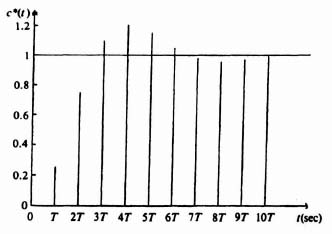
Figure 4.42 Response of the systems shown in Figure 4.38 to a unit-step input, where T = 1.43.
4.11. BODE AND ROOT-LOCUS DIAGRAMS FOR DISCRETE TIMESYSTEMS USING MATLAB [13]
The control-system engineer has much flexibility in converting between continuous time to discrete time, and obtaining the Bode and root-locus diagrams for discrete time systems using MATLAB, the professional Control System Toolbox, and the AMCSTD Toolbox.
A. Conversion between Continuous and Discrete Time
The AMCSTD Toolbox has a very useful utility for converting between continuous and discrete time, and accomplishing the bilinear transformation. This utility is denoted as “polysbst.” Its application in going from G(z), as given by Eq. (4.174), to G(w), as given by Eq. (4.178), will next be illustrated:
POLYSBST: Substitute the variable of a polynomial with another polynomial
function [newnum] = polysubt (num, subnum);
function [newnum, newden] = polysubt (num, den, subnum, subden);
Substitute the variable in the original polynomial (num or num/den) with a polynomial expression (subnum or subnum/subden). The result is returned as a polynomial (newnum or newnum/newden).
Using G(z) = (T*2/2)(z + 1)/(z − 1)2 and T = 0.26 from Eq. (4.174), given G(w) = (1 − w)/7.69)/w2 as shown in Eq. (4.178):
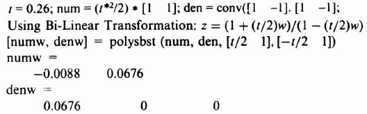
which simplifies to G(w) = (1 − w/7.69)/w2 as shown in Eq. (4.178).
The Control Toolbox accommodates many types of conversions:
C2DM (or C2D) allows conversion from continuous to discrete domain.
D2CM (or D2C) allows conversion from discrete to continuous domain.
With the Control System Toolbox, this would be accomplished using D2CM:
[numw,denw] = d2cm (num,den,t,‘tustin’)
The resulting output from the Control System Toolbox would be:
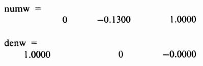
This simplifies to G(w) = (1 − w/7.69)/w2 as shown in Eq. (4.178).
B. Bode Diagram
The application and use of the Bode diagram for discrete control systems is the same as for continuous systems, except that we have to convert from the z-domain to the w-domain, and the frequency in the discrete time case is the fictitious frequency “ν” where w = jν. Otherwise, the Bode diagram is drawn the same, and phase and gain margins have the same interpretation. Therefore, everything stated in Section 1.7 for obtaining the Bode diagram of continuous systems using MATLAB is valid here too for discrete-time systems.
C. Root-Locus Diagram
The construction of the root-locus diagram for discrete time systems is the same as for continuous systems. Therefore, everything stated in Section 1.7 for generating the root-locus diagram for continuous sytems is valid here too for discrete-time systems. The primary difference is in the interpretation of the root locus for discrete-time systems. We have shown in Section 4.10 that the unit circle in the z-plane defines the region of stability, as compared to the imaginary axis of the s-plane for continuous systems. The AMCSTD Toolbox has the following special functions which are great aids in constructing and analyzing the root locus for discrete-time systems:
- rlaxis determines portions of the real axis that are part of the root locus.
- rlpoba determines the points of breakaway and break-in, and the values of gain at these points.
- rootmag is especially useful in the use of the root locus for discrete-time systems. It determines gain and values of the roots at a particular distance from the origin of the z-plane. This is particularly useful in finding the gain and root values when the root locus crosses the unit circle which is the stability boundary for discrete systems.
- rootangl determines the gain and values of the roots at a particular angle from the origin.
4.12. RAGAZZINI'S METHOD
A very useful method for the design of sampled-data control systems is Ragazzini's method [2, 7]. Unlike other approaches for analysis and design, such as the Bode diagram (in the w-plane) and the root locus which was extended from continuous systems to discrete systems, Ragazzini's method was developed specifically for the design of sampled-data control systems.
Let us next consider stabilizing a sampled-data control system by means of a digital controller, as is illustrated in Figure 4.43. The object of this device is to compute a sequence of output numbers ![]() , which are linearly related to the input number sequence
, which are linearly related to the input number sequence ![]() , in order to obtain a desired system response. The digital controller may contain active elements or simple passive networks. When this device contains active elements, the control engineer is completely free in choosing any stabilizing function in order that the desired system response may be obtained. The procedure for finding D(z) is known as the direct design method of Ragazzini [2, 7].
, in order to obtain a desired system response. The digital controller may contain active elements or simple passive networks. When this device contains active elements, the control engineer is completely free in choosing any stabilizing function in order that the desired system response may be obtained. The procedure for finding D(z) is known as the direct design method of Ragazzini [2, 7].
We shall assume that the digital controller is a linear device. Therefore, the output and input number sequences are related linearly. The linear relationship which exists between the input and the output sequence, ![]() and
and ![]() , respectively, can be expressed as
, respectively, can be expressed as
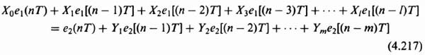
where Xl, and Ym represent constant terms. The z transform of this equation can be written as
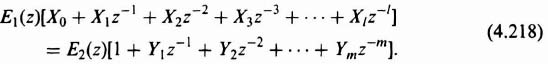
The z transfer function of the digital controller, D(z), is defined as

From Eq. (4.218), D(z) can be expressed as

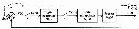
Figure 4.43 Sampled-data control system utilizing digital controller compensation.
In order that the digital controller be physically realizable, the denominator of Eq. (4.220) must contain the term 1.
For the system in Figure 4.43, the system transfer function H(z) can be expressed as

The term G(z) is the z transform corresponding to the Laplace transfer function G1(s)G2(s). In order that a specified system transfer function H(z) may be realized, the various constants of D(z) must be appropriately chosen. From Eq. (4.221) the value of D(z) corresponding to a specified value of H(z) is given by
It is important to realize that the primary purpose of the digital controller is to cancel any undesirable poles and zeros of the uncompensated system and replace them with poles and zeros which will result in a desired system reponse. It is obvious from Eq. (4.221) that this can be accomplished by designing D(z) in order that its zeros correspond to the poles of G(z) and its poles correspond to the zeros of G(z), which lie on or outside the unit circle of the z-plane. However, it has been shown that this method of compensation is not practical because any slight change in the parameters of D(z) or G(z) may result in having the poles and zeros of G(z), lying on or outside the unit circle of the z-plane, being uncanceled [7].
A better method for compensation may be obtained by considering Eq. (4.222). Poles and zeros of G(z) that lie on or outside the unit circle in the z-plane, may be canceled by specifying 1 − H(z) and H(z) in order that they cancel the poles and zeros, respectively. The following four rules must be pursued when specifying a system transfer function H(z), which will result in a stable system:
- The specified system transfer function H(z) must contain as its zeros all the zeros of G(z) that lie on or outside the unit circle in the z-plane.
- 1 − H(z) must contain as its zeros all of the poles of G(z) that lie on or outside the unit circle in the z-plane.
- In order that D(z) be physically realizable (causal), it should not have a pole at infinity as z → ∞. Therefore, from Eq. (4.222) if G(z) has a zero at infinity, it is necessary that H(z) have a zero there, too, in order to prevent D(z) from having a pole at infinity.
- H(z) must be specified in order that the steady-state error, resulting from the application of an input having the form
is zero. From Table 4.1, this type of input can represent a step, ramp, acceleration, etc., depending upon the value of m. A(z) represents a polynomial in z−1 which does not contain factors of the form 1 − z−1. From the relationships given by
and
the z transform of the system error can be expressed as
Applying the final-value theorem (see Eq. (4.61)), to Eq. (4.226), we obtain
Substituting Eq. (4.223) into Eq. (4.227) the following expression results:
It is easily seen from Eq. (4.228) that the steady-state error, for inputs of the form given by Eq. (4.223) will be zero if 1 − H(z) satisfies the relationship
where F(z) is an unspecified ratio of polynomials in z−1 and m is the order of the denominator of the input, R(z). When F(z) is unity, a “minimal prototype” response function results and the order of H(z) in z−1 is a minimum. However, a minimal prototype response function can only be utilized when H(z) does not contain any zeros on or outside the unit circle of the z-plane. A little further thought reveals that a system in which m = 1 will respond to a unit step with zero steady-state error, and when m = 2 it will respond to a unit ramp with zero-state error, etc. In addition, a system utilizing a minimal prototype will respond with zero steady-state error to lower-order input functions.


We shall next apply the theory developed to several systems of the types shown in Figure 4.43, where the data extrapolator is a zero-order hold. The sampling rate will be assumed equal to 1 sec. The techniques used to choose the value of D(z) and the system's response to various inputs will be illustrated.
A. Example of Ragazzini's Method when the Proces G2(s) is an Integrator
Consider a system which has a process that is an integrator:
1. Design of D(z). The first step of the procedure is to determine the z transform G(z), corresponding to the Laplace transfer function given by
From Table 4.1,

Examination of G(z) shows that it contains a permissible pole at z = 1. Applying rule numbers 1 and 3, we can specify the system transfer function as
Assuming that zero steady-state error to a unit step input is desired, the following relationship is obtained from rule 4, Eq. (4.229):
From rule number 4, F(z) is set equal to 1 to obtain a minimal prototype system. Therefore, Eq. (4.234) can be expressed as
Substituting Eq. (4.233) into Eq. (4.235) we obtain
From Eq. (4.236) the solution for K1 is
Substituting Eq. (4.237) into Eq. (4.233), we obtain
It is now possible to compute the value of D(z). Substituting Eq. (4.232) and (4.238) into Eq. (4.222), we obtain
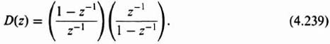
This expression reduces to
2. System Response to a Unit Step. The z-transfer function of the system is given by

From Table 4.1, the z transform of a unit step input
By substituting Eqs. (4.238) and (4.242) into Eq. (4.241) the z transform of the output response is obtained. The resulting expression is

By expanding Eq. (4.243) into a power series in z, and then taking the inverse z transform, the output response can be sketched. The result is
or
and is plotted in Figure 4.44. Observe that this system follows a unit step input with zero steady-state error based on our previous choice of 1 − H(z) in accordance with rule 4.
B. Example of Ragazzini's Method when the Process G2(s) is a Double Integration
The next system we will consider contains a process which is a double integrator and may be represented by the transfer function
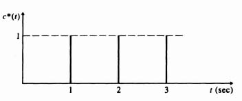
Figure 4.44 Response of the system shown in Figure 4.43 containing a zero-order hold and an integrating process, designed in accordance with Ragazzini's method, to a unit step input.
1. Design of D(z). Utilizing the same procedure that was followed in the previous problem, we will first obtain G(z). The expression for G(s) is

Utilizing Table 4.1, we obtain the z transform as
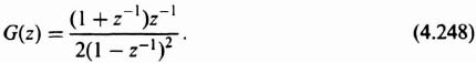
Examination of G(z) shows that it contains a zero at z = −1 and two poles at z = 1. Applying rule numbers 1 and 3, we can specify the system transfer function as
Assuming that zero steady-state error to a unit ramp is desired and we wish to cancel the two poles of G(z) at z = 1, the following relationship is obtained from rules 2 and 4:
Observe from rule 4 that this expression automatically insures that the system will respond to a unit ramp with zero steady-state error. However, a minimal prototype response function cannot be specified, because G(z) contains a zero on the unit circle in the z-plane. Instead, a larger minimum finite settling response time will be obtained. Therefore Eq. (4.250) can be rewritten as
Substituting Eq. (4.249) into Eq. (4.251), we obtain the expression
Here γ2, γ3, etc., will be considered to be zero in order to obtain a solution for the constants of the equation. Equating coefficients of terms having the same power of z together, we then obtain three simultaneous equations, relating the constants of Eq. (4.252), If γ2, γ3, etc., were considered, then we would have more unknowns than equations and we would obtain a non-minimum finite settling time. The results are as follows:
Substituting Eq. (4.253) into Eqs. (4.249) and (4.251), we obtain
It is now possible to compute the value of D(z). Substituting Eqs. (4.248), (4.254), and (4.255), into Eq. (4.222) we obtain the expression
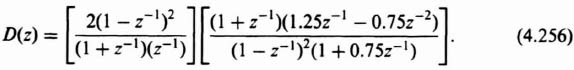
This expression can be reduced to

2. System Response to a Unit Step. By substituting Eqs. (4.242) and (4.255) into Eq. (4.241) the z transform of the output response can be obtained. The resulting expression can be reduced to
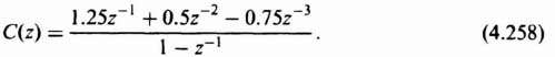
By expanding Eq. (4.258) into a power series in z and then taking the inverse z transform, the output response can be obtained. The result is
or
and is shown in Figure 4.45. Notice that the steady-state error of this system to a unit step input is zero. This is what we should expect based on our previous choice of 1 − H(z) in accordance with rule 4.
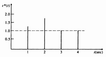
Figure 4.45 Response of the system shown in Figure 4.43 containing a zero-order hold and a double integrating process, designed in accordance with Ragazzini's method, to a unit step input.
3. System Response to a Unit Ramp. From Table 4.1, the z transform of a unit ramp is given by the expression

Becuase we are assuming a sampling time of 1 sec, Eq. (4.261) can be reduced to

By substituting Eqs. (4.255) and (4.262) into Eq. (4.241), the z transform of the output response is obtained. The resulting expression can be reduced to
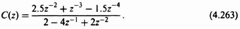
By expanding Eq. (4.263) into a power series in z and then taking the inverse z transform, the output response can be obtained. The result is
or
and is plotted in Figure 4.46. Notice that the steady-state error of this system to a unit ramp input is zero because of our choice of 1 − H(z) based on rule 4.
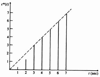
Figure 4.46 Response of the system shown in Figure 4.43 containing a zero-order hold and a double-integrating process, designed in accordance with Ragazzini's method, to a unit ramp input.
A comparison of Figures 4.45 and 4.46 indicates that the system responds relatively smoothly to the type of input it was designed for, specifically a ramp, and poorly for lower-order inputs such as a step. For example, it exhibits an overshoot of 75% when responding to a step input before finally settling to its steady-state value. It is interesting to note that in the previous example, which consisted of a sampled-data system containing a single integrator, the response did not exhibit an overshoot to a step input because we originally designed it to respond specifically to this type of input.
C. Damping Effect of the Staleness Factor
A method of overcoming the severe overshoots of sampled-data control systems to inputs that are of a lower order than they are specifically designed for is to introduce a term to the system transfer function known as the “staleness factor.” Implementation of this factor results in softening the system's response to a wide variety of inputs. The staleness factor term is added to the original system transfer function in the following manner:
where H(z) = original z-transfer function of the system, Hs(z) = z-transfer function of system with the staleness factor term added, C = staleness factor constant whose value ranges from + 1 to −1 for stable systems, and N = exponent which can be any positive value.
Because Bertram [14] has shown that not very much is gained by designing N greater than unity, we shall assume that N = 1. The value for the staleness factor, C, can be chosen by analytical optimizing procedures or by laboratory trial-and-error techniques. Generally, it can be stated that as C approaches unity, maximum damping is produced, and as C approaches zero, the damping is decreased. We shall illustrate the damping effect of the staleness factor term upon the response of the sampled-data control system considered previously (control system of Figure 4.43 where G2(s) is a double integration) by introducing a staleness factor of 0.3 and comparing the system's response with that illustrated in Figures 4.45 and 4.46.
1. Design of D(z). Utilizing the same procedure that was followed previously, we shall first compute the value of D(z). The introduction of the staleness factor term,
![]()
modifies Eq. (4.249) and (4.251) as follows:


Substituting Eq. (4.267) into (4.268), we obtain the expression

As in the previous example, the constants γ2, γ3, etc., need not be considered. Equating coefficients of terms having the same power of z together, we obtain three simultaneous equations relating the constants of Eq. (4.269). The results are as follows:
Substituting Eq. (4.270) into Eq. (4.267) and (4.268), we obtain

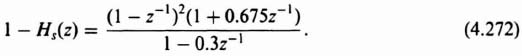
The value of D(z) can now be computed by substituting Eqs. (4.248), (4.271) and (4.272) into Eq. (4.222). The resultant expression is
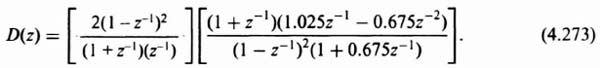
This can be reduced to

A comparison of Eqs. (4.257) and (4.274) shows that the values of the various coefficients are different but that the complexity of the digital controller is the same. Therefore, the introduction of the staleness factor term may be obtained by merely readjusting the programming of the digital controller and does not require a more complex device.
2. System Response to a Unit Step. By substituting Eqs. (4.242) and (4.271) into Eq. (4.241) the z transform of the output response is obtained. The resulting expression can be reduced to
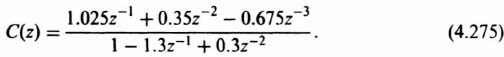
By expanding Eq. (4.275) into a power series in z and then taking the inverse z transform, the output response can be obtained. The result is
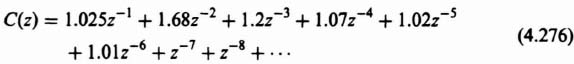
or

and is sketched in Figure 4.47. Comparing Figures 4.45 and 4.47, we can clearly see the damping or “softening” effect of the staleness factor upon the system's response. The maximum percent overshoot is reduced from 75% to 68%. By varying C between ±1, an optimum value can be found.
3. System Response to a Unit Ramp. The z transform of the output response to a unit ramp input can be obtained by substituting Eqs. (4.262) and (4.271) into Eq. (4.241). The resulting expression can be reduced to
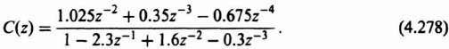
By expanding Eq. (4.278) into a power series in z and then taking the inverse z transform, the output response can be obtained. The result is
or


Figure 4.47 Use of the staleness-factor term for softening the response of a system containing a zero-order hold and a double-integrating process to a unit step input.
and is plotted in Figure 4.48. Comparing Figures 4.46 and 4.48, we can clearly see the damping or softening effect of the staleness factor upon the system's response. Although it is true that the implementation of the staleness factor term results in the system taking a little longer to respond to a ramp input, it must be remembered that this solution is a compromise which enables the system to respond less sharply to a step input.
4.13. THE DIGITIZATION PROCESS AND THE DESIGN OF DIGITAL FILTERS [2]
Up until this chapter on digital control-system analysis and design, the analysis and design has focused on continuous or analog control systems. When compensating networks were determined in Chapters 2 and 3 for linear continuous control systems, the resulting compensating network's form was either continuous or analog. In practice, however, we know that the control system will be implemented digitally. Therefore, how do we digitize the resulting continuous (or analog) compensating network? That is the subject of this section.
Let us consider the control system illustrated in Figure 4.49. We wish to implement the continuous (or analog) form of D(s) digitally by obtaining D(z) so that D(z) duplicates the phase and amplitude characteristics of D(s) as closely as possible. However, we must recognize that D(z) cannot exactly duplicate the phase and amplitude characteristics of D(s) because D(s) acts on the complete time history of E(s) while D(z) only acts upon the samples of E(s).
Figure 4.48 Use of the staleness-factor term for softening the response of a system containing a zero-order hold and a double-integrating process to a unit ramp input.

Figure 4.49 A continuous (or analog) control system.
There are many digital approximations to this problem. For example, one approach is that of numerical integration. This is illustrated in Problem 4.41 which illustrates numerical integration by summing rectangles over a continuous function. Problem 4.42 illustrates numerical integration by summing trapezoidal areas under a continuous function. Both methods result in a z-transform transfer function relating E(z) and U(z), D(z), whose phase and amplitude characteristics are very close to that of D(s).
We will focus attention in this section on the practical matched pole-zero method which is based on the relation between the s- and z-planes given by Eq. (4.32).
The procedure is to obtain the z transform of the sampled function of the continuous transfer function D(s) and relate the poles of D(z) to the poles of D(s) according to Eq. (4.281). The same reasoning is applied to the zeros of D(z) and the zeros of D(s). The rules of the matched pole-zero method are as follows
Rule 1. Match all poles and zeros of D(s) and D(z) according to Eq. (4.281). For example, if D(s) has a pole at s = −2, then D(z) has a pole according to z = e−2T.
Rule 2. Match the gain of D(s) and D(z) at a critical frequency. Usually, the critical frequency selected is dc. Therefore, for this case we match the gains of
Rule 3. Add (1 + z−1)n as appropriate only if the numerator is of lower order that of the denominator. This has the effect of mapping zeros of D(s) at s equals infinity to the point z equals minus one for D(z).
Let us illustrate the matched pole-zero with an example. It is assumed that the compensating network, D(s), in Figure 4.49 represents a phase-lead network designed to add 36.88° phase lead at a critical frequency of ω1 = 1 rad/sec:
It will also be assumed that the sampling time that the digitized network will operate at is 0.5 sec. Following the three rules presented, D(z) is obtained as follows
Rule 1. Pole at s = −2 transforms into the z-plane as
Therefore, the corresponding pole in the z-plane is (z − 0.37).
Zero at s = −0.5 transforms into the z-plane as
Therefore, the corresponding zero in the z-plane is (z − 0.78).
Rule 2. The gain of D(z) is made to match the gain of D(s) at de:
The gain of D(s) at dc is:
Therefore,

Therefore,
Combining the results of Eqs. (4.284), (4.285), and (4.289), D(z) is given by
The next question to answer is whether the resulting digitized network, D(z), is stable from the resulting pole and zero plot shown in Figure 4.50. The location of the pole illustrated in this figure shows that D(z) is stable.
The last step of the design is to determine the phase shift and amplitude characteristics resulting from the digitized network D(z) and compare it with that of the continuous network D(s) at the critical frequency of ω1 = 1 rad/sec, To determine this for the digitized network D(z) of Eq. (4.290), we must first determine z corresponding to the critical frequency ω1 = 1 rad/sec and the sampling time T = 0.5 sec.
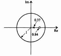
Figure 4.50 Location of pole and zero of ![]()
Since
then
Substituting Eq. (4.293) into Eq. (4.290), we obtain the following:

Equation (4.294) can be simplified to the following:
Therefore, this method gives a very close fit between the phase of D(s) and D(z) at 1 rad/sec, and an exact amplitude fit at dc.
The resulting difference equation, which must be programmed into the digital computer, is obtained from Eq. (4.290) as follows:
Therefore,
or,
The resulting digital control-system version, corresponding to the continuous (or analog) version of Figure 4.49 is illustrated in Figure 4.51.
There are several other methods that can be used to digitize a continuous (or analog) network. We have mentioned the numerical integration methods which are presented in Problems 4.41 and 4.42. Another more sophisticated method is the hold equivalence method which is discussed in Reference 13. Based on my experience, I prefer to use the matched pole-zero method. It is very simple to use and usually provides very close matches between the continuous (or analog) network and the digital case.

Figure 4.51 Digital control system corresponding to the continuous (or analog) version of Figure 4.49.
4.14. SUMMARY
This chapter has extended the concept of linear continuous system analysis and design, presented in the first eight chapters of this book, to digital control systems. Sampling characteristics were analyzed in the time and frequency domains. The use of zero-order and first-order holds for digital-to-analog conversion in sampled-data systems were presented and analyzed. The use of z-transform theory was presented for simplifying the analysis of discrete systems. Its use permitted the analysis of digital control systems using techniques similar to those used for continuous systems. For example, Mason's signal-flow graph and theorem were equally applicable to the analysis of sampled-data block diagrams.
The concept of stability in the z-plane was presented, where the unit circle in the z-plane was shown to be analogous to the imaginary axis in the s-plane for stability analysis. Three mathematical tests were analyzed: modified Routh–Hurwitz, Schur–Cohn, and Jury's stability criteria. The modified Routh–Hurwitz criterion in the w-plane was very similar to the conventional Routh–Hurwitz criterion used for continuous systems in the s-plane. The Schur–Cohn and Jury tests were unique to discrete systems. Both the Bode diagram and the root-locus concepts for continuous system analysis and design, presented in Chapter 1 and Chapter 2, were extended to discrete systems. By the use of the w transform for the Bode diagram, we were able to use analysis techniques similar to those used for continuous systems in the s-plane. We found that all the rules of root-locus construction for continuous systems in the s-plane, presented in Section 6.14‡, were also valid for discrete systems in the z-plane. The design methods used in this chapter for discrete systems using the Bode and root-locus methods relied on the techniques presented in Chapter 2 for continuous systems. We concluded the design methodology for discrete systems with Ragazzini's direct design method, which is a technique unique to discrete systems.
It is important for the control-system engineer to be able to think and be adept from the dual continuous and discrete-system viewpoints. This capability was emphasized in this chapter, as we related the techniques presented in this chapter on digital control systems to those of the continuous world presented previously in this book. As digital computer control systems are becoming increasingly prevalent in industrial and military applications, the control-system engineer should find the techniques presented in this chapter very useful in practice.
A complete design case study of a sampled-data control systems for controlling the temperature of a liquid in a tank is presented in Section 7.6. The system uses a microcomputer to control the position of a solenoid valve, which then controls the quantity of steam into the tank coil. In this way, the microcomputer controls the temperature of the liquid contained in the tank. This is an interesting problem that integrates the various procedures illustrated in this chapter into a practical design example.
4.15. IUUSTRATIVE PROBLEMS AND SOLUTIONS
This section provides a set of illustrative problems and their solutions to supplement the material presented in Chapter 4.
- I4.1. A sinusoidal function
is sampled every T = 0.2 sec. Determine the z transform of the resultant sampled sequence.
SOLUTION: From item 11 of Table 4.1:
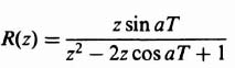
For this problem, T = 0.2, a = 4, and we must multiply this expression by 2. Therefore:
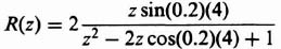
Therefore:

This expression can be simplified to the following:

- I4.2. Determinte the z transform for the following:

SOLUTION: Using partial fraction expansion of F(s), we obtain the following:
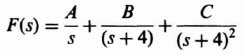
where the constants are given by the following:
Therefore,
From Table 4.1, we find the z transform of this expression to be:

- I4.3. Determine the z transform of the function r(t) drawn in the following figure. Assume that the sampling period is one second.

SOLUTION: y(t) = t − (t − 2)U(t − 2), t ≥ 0.
Therefore,
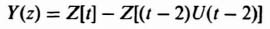
From Table 4.1, we have:
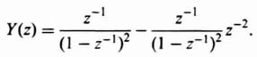
Therefore, the z transform of y(t) is given by:
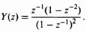
- I4.4. The z transform of a sampled-function, r(t), is given by:
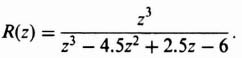
Determine the z transform of r(t − 3T)U(t − 3T).
SOLUTION:
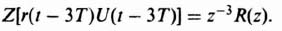
Therefore, the z transform of r(t − 3T)U(t − 3T) is given by:
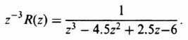
- I4.5. Determine the inverse z transform of

using:
- Partial fraction expansion.
- Power series expansion.
How do your results compare?
SOLUTION:
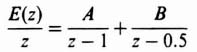
where
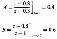
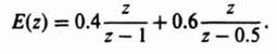
From Table 4.1, the inverse z transform of E(z) is given by:
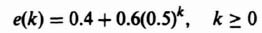
- The z transform of E(z) can be written as:

Dividing denominator into numerator, we obtain the following:

This is the series form corresponding to the closed-loop form obtained in part (a). The results in parts (a) and (b) are in agreement.
- I4.6. The difference equation representing a digital process is given by the following expression:

where

- Determine C(z).
- Determine c(k) from finding the inverse z transformation of C(z).
- Find c(100,000).
SOLUTION:
- the z transform of the given difference equation is given by:
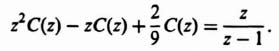
Solving for C(z), we obtain the following:

- Using partial fraction expansion, we obtain the following:

where
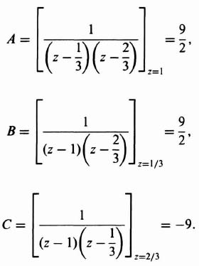
Therefore, C(z) is given by:

The inverse z transform of C(z) can be obtained from Table 4.1 as follows:
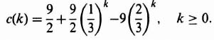
-

- I4.7. The difference equation representing a digital process is given by the following expression:

where
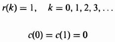
Determine c(k).
SOLUTION:

Solving for C(z), we obtain:
C(z) can be expanded into partial fractions as follows:

where
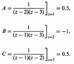
Therefore,
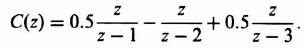
Using Table 4.1, the inverse z transform of this equation is given by:
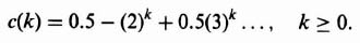
- I4.8. A system can be represented by the following,

where K represents the system gain. Determine the z-transform transfer function, C(z)/R(z), of this difference equation.
SOLUTION:
Therefore, the transfer function, C(z)/R(z) is given by:

- I4.9. The transfer function of a linear, time-invariant discrete-data system is unknown. To determine its transfer function,

it is subjected to an input sequence given by

The resulting output is modeled by the following sequence:
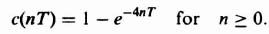
Determine the transfer function G(z).
SOLUTION:
From Eq. (4.30):
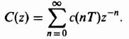
Therefore,
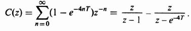
This can be simplified to:


then, the transfer function, G(z), is given by:
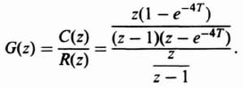
Therefore,

- I4.10. A sinusoidal signal of 6 Hz is applied to an ideal sampler and zero-order hold combination where the sampling rate is 10 Hz. Determine all frequencies present in the output which are less than 50 Hz.
SOLUTION:
Output components Frequencies at output (Hz) f1 6 f1 − f1 4 fs + f1 16 2fs − f1 14 2fs + f1 26 3fs − f1 24 3fs + f1 36 4fs − f1 34 4fs + f1 46 5fs − f1 44 - I4.11. The responses of two open-loop control systems to an exponential input, r(t) = e−t U(t), are to be compared.
- Determine c(nT) for the system shown in Figure I4.11a. Carry your answer out to the first four sampling instants.
- Repeat part (a) for the continuous control system shown in Figure I4.11b, and determine c(t) at these same first five sampling instants.
- From your results in parts (a) and (b), compare the outputs of these two systems. Explain any differences.
SOLUTION:
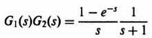
By means of partial-fraction expansion, this can be written as

(This agrees with Eq. (4.118) in Section 4.6 of this book.) The z transform of this expression can be obtained from Table 4.1 by inspection as follows:
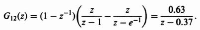
Therefore,

Dividing the denominator into the numerator, we obtain the following senes:


By utilizing Table 4.1, the inverse z transform can be expressed as


From inspection of Appendix A, eighth item (for n = 2), the inverse Laplace transform is given by:

Therefore, in terms of this function sampled every second, we can write this as
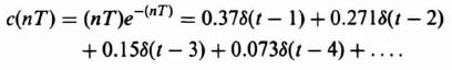
- The values of c(nT) in parts (a) and (b) differ because the input energy to

is different in parts (a) and (b) of this problem.
- I4.12. An open-loop digital control system containing a sampler whose sampling time is 1 Hz, a digital filter, a zero-order hold, and a process is illustrated:
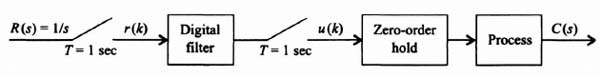
Assume that the digital filter solves the following difference equation:

The transfer function of the process is given by

Determine the transfer function, C(z)/R(z).
SOLUTION: The z transform of the difference equation is given by
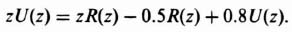
Therefore, the z-transform transfer function of the digital filter is given by

The z transform of the zero-order hold and the process is given by
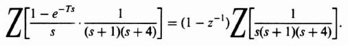
Using partial fraction expansion, we obtain the following z transform for the zero-order hold and the process:

Therefore,

- I4.13. Determine the transfer function C(z)/R(z) for the discrete-data control system illustrated. Assume that the sampling period is one second.

SOLUTION: From Problem I4.12, the z transform of G1(s) and G2(s) is given by

Therefore,
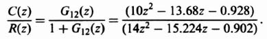
- I4.14. Determine the form of the transient response of discrete-time systems whose characteristic equations are given by:
- z2 − 1.5z + 0.56 = 0.
- z2 − 0.49 = 0.
- z2 − 1 = 0.
- z2 − 1.3z + 0.36 = 0.
SOLUTION:
- I4.15. A digital control system is described by the difference (or state) equation given by

where r(n) represents the input and x(n) represents the state variable. Determine the value of K for the system to be stable.
SOLUTION: Taking the z transform of this difference (or state) equation, we obtain:
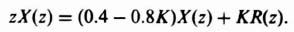
Therefore, the transfer function, X(z)/R(z) is given by:
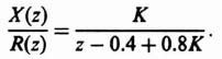
The resulting characteristic equation is given by:
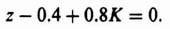
The root of this characteristic equation is given by
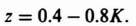
For stability, it is necessary that

or

Therefore, for stability, it is necessary that

- I4.16. A unity-feedback digital control system has a forward transfer function given by
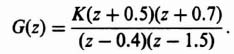
The Nyquist diagram in the GH(z) plane for a specific value of gain K is illustrated.

- Determine the value of gain K that this Nyquist diagram is drawn for.
- Determine the location of point “x.”
- Is the system stable?
- At z = −1:
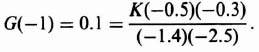
Solving for K:

- At z = 1:
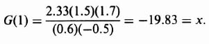
- N = Z − P
where N = −1 because there is one counterclockwise encirclement of the −1, 0 point, and P = 1 because there is one pole of GH(z) outside the unit circle at z = 1.5. Therefore,
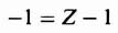
Therefore, Z = 0 and the system is stable.
- I4.17. We wish to analyze the performance of a unity-feedback sampled-data control system whose forward transfer function, Gp(s), is given by

and it contains a zero-order hold and a sampler whose sampling frequency will be designed to be one-hundredth of the gain crossover frequency.
- Determine the gain crossover frequency, ωc analytically without using the graphical Bode plot.
- Determine the phase margin and gain margin of this control system analytically without using the graphical Bode plot.
- A phase-lead network compensation, Gc(s), given by
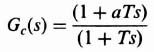
is to be added in series with the process' transfer function, Gp(s). Determine the values of a and T in order that the zero factor of Gc(s) cancels the pole of Gp(s) at s = −10, and the damping ratio is unity.
- Determine the gain crossover frequency, ωc analytically without using the graphical Bode plot.
- Determine the phase margin and gain margin of this control system analytically without using the graphical Bode plot.
- This system can be approximated and analyzed as a continuous system because the sampling frequency is so fast compared to the gain crossover frequency (see Figure 4.9). Therefore,
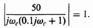
Therefore,


Therefore, the phase margin, γ, is given by

The gain margin is infinity.

Therefore, it is necessary that

so that the zero factor of Gc(s) cancels the pole of Gp(s). Therefore,

The transfer function of the closed-loop system is given by:
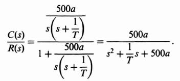
Comparing this equation with that of Eq. (B.3), we obtain the following:
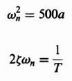
where the damping ratio ζ = 1 (given). Solving these two equations simultaneously, we obtain the following:

Therefore, the phase-lead compensation network is given by:
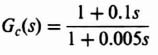
and
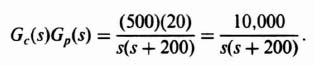
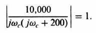
Therefore,

Therefore,


Therefore, the phase margin, γ, is given by:
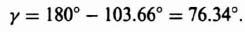
The gain margin equals infinity.
- I4.18. A sampled-data control system is shown in Figure I4.18(i). It contains a first-order hold G1(s), and a process G2(s) where
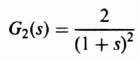
and the sampling time, T, is 1 sec.

- Draw the Bode diagram of this sampled-data control system, and determine the gain crossover, phase margin, gain margin, and the phase crossover frequency.
- A minimum phase margin of 65°, and a minimum gain margin of 6.5 dB are desired. Determine the gain reduction required to achieve these design values.
SOLUTION:

The z transform of this expression is given by
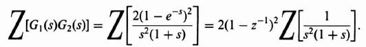
The partial-fraction expansion of the last bracketed term is given by
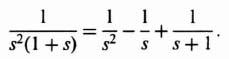
Therefore, the z transform of G1(s)G2(s) is given by

Using Eq. (4.175) with T = 1 sec, we obtain the following relationship between the z- and the w-planes:
Substituting (I4.18-2) into Eq. (I4.18-1), we obtain the following:

The resulting Bode diagram is shown in Figure I4.18(ii). It shows that the gain crossover frequency = 1.6197 rad/sec, the phase margin = 49.2689°, the gain margin = 5.5387 dB, and the phase crossover frequency = 3.5211 rad/sec.
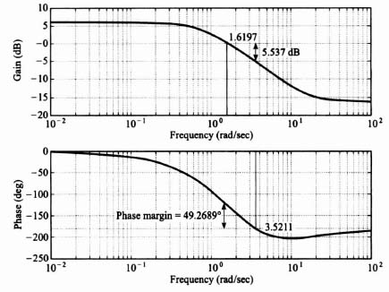
- When the gain is reduced from 2.02 to 1.78, we achieve the following: gain crossover frequency = 1.3079 rad/sec; phase margin = 65°; gain margin = 6.83 dB; phase crossover frequency = 3.5211 rad/sec (see Bode diagram in Figure I4.18(iii)).

- I4.19. The performance of the following digital control system is to be determined from knowledge of the root locus:
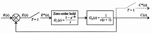
- Determine the z transform of the open-loop system.
- Determine the closed-loop transfer function, C(z)/R(z).
- Determine and locate in the z-plane the closed-loop poles.
- Determine the damping ratio of this closed-loop control system from knowledge of the exact location of the roots and by using Figure 4.40.
- Determine the damping ratio of a comparable analog control system in which the sampler and zero-order hold are removed.
- What conclusions can you reach by comparing your results in parts (d) and (e).
SOLUTION:

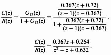
- The characteristic equation is given by

Therefore, the roots are located in the z-plane at

- From Figure 4.40, the damping ratio equals 0.25.

Setting like coefficients toether, we obtain the following two simultaneous equations to solve:

Solving these two equations simultaneously, we obtain
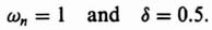
- The analog version of this control system, which does not contain the sampler and zero-order hold, has a damping ratio of 0.5. The digital version has a damping ratio of 0.25. The sampler and zero-order hold have the effect of increasing the phase lag in the control system, decreasing its relative stability, and decreasing its damping ratio.
- I4.20. A sampled-data control system is shown in Figure I4.20(i). It conains a zero-order hold G1(s), and a process G2(s) where
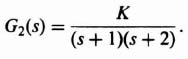
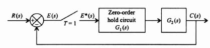
- Draw the root locus of this sampled-data control system and find Kmax if the sampling time, T, is 1 sec.
- The value of Kmax can be increased if the sampling time is made faster. Draw the root locus of this sampled-data control system if the sampling time, T, is halved to 0.5 sec and find Kmax for this system.
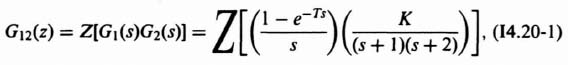
The root-locus plot for this part is shown in Figure I4.20(ii). It was obtained using MATLAB, and shows that Kmax equals 12.44 at a break-in point located at s = −0.9914, 0.
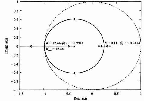
Figure I4.20(ii) Root locus for the case where the sampling time = 1 sec.
- With a sampling rate of 0.5 sec, Eq. (I4.20-2) is modified to the following:
Therefore,
The root-locus plot for this part is shown in Figure I4.20(iii). It was obtained using MATLAB, and shows that the system is stable for the following conditions:

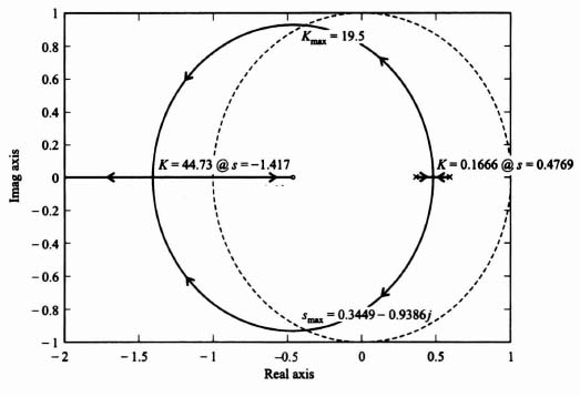
Figure I4.20(iii) Root locus for the case where the sampling time = 0.5 sec.
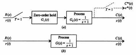

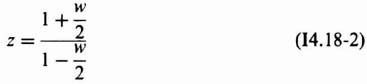
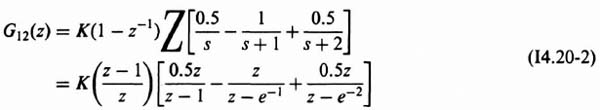


PROBLEMS
- 4.1. Prove item 8 of Table 4.1.
- 4.2. Prove item 12 of Table 4.1.
- 4.3. Find the z transform of

- 4.4. Determine the z transform of
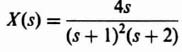
by using the partial fraction method.
- 4.5. Determine the z transform in closed form for the following function:

- 4.6. Determine the inverse z transform of

using:
- Partial fraction expansion.
- Power series expansion.
How do your results compare?
- 4.7. Determine the inverse z transform of
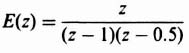
using:
- Partial fraction expansion.
- Power series expansion.
- 4.8. A triangular input, r(t) is applied to the low-pass filter shown in Figure P4.8.
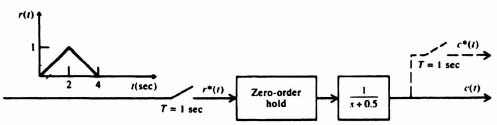
- What is the z transform of r*(t)?
- What is the z transform of c*(t)?
- Find c*(t).
- Apply the initial- and final-value theorems to obtain c(0) and c(∞), respectively.
- 4.9. Repeat Problem 4.8 if the input r(t) is given by the waveform shown in Figure P4.9.
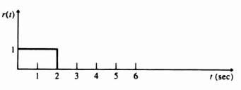
- 4.10. Determine the z transforms corresponding to the following transfer functions:
- 4.11. Determine the value of c(k) for the following difference equation by using the z-transform method:
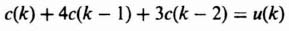
where
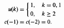
- 4.12. The difference equation representing a digital process is given by the following expression:

where
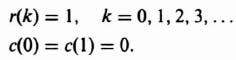
Determine c(k).
- 4.13. Derive the z transform of the output, C(z), for the sampled-data feedback control systems shown in Figure P4.13.

- 4.14. Determine the transfer function C(z)/R(z) for the system shown in Figure P4.14.

4.15. A second-order digital filter having the configuration shown in Figure P4.15 is to be designed:
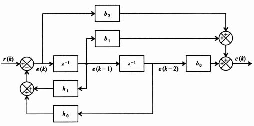
It is desired that the z-transform transfer function of this filter should be:
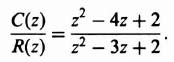
- Determine the values of the coefficients b1, b1, b2, h1, and h1 to satisfy the desired filter's transfer function.
- Determine the two difference equations required to describe this second-order digital filter. [Hint: Write one difference equation at e(k) in terms of r(k), e(k − 1), and e(k − 2); write the second difference equation at c(k) in terms of e(k), e(k − 1), and e(k − 2)].
- 4.16. The linear system shown in Figure P4.16 is subjected to an input which is sampled and held by a zero-order holding circuit. Assume that the impulse sampling approximation is applicable, and that the sampling interval T, is 1 sec.
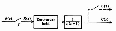
- Determine the z transfer function relating the sampled input R(z) and the sampled output C(z).
- For a step function at the input R(s), determine the z transform of the output C(z). Sketch the impulse sequence, c*(t).
- For a unit-ramp input, determine the z transform of the output C(z). Sketch the impulse sequence c*(t).
- 4.17. Repeat Problem 4.16 if the sampling interval is changed to 0.1 and 10 sec.
- 4.18. The system in Figure P4.18 is to be analyzed.
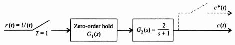
- Determine the value of G(z) = G12(z).
- Determine the value of C(z) for a unit step input at R(z).
- Determine the value of c*(t).
- Determine the value of c(O) using the initial-value theorem. Check your answer from your result in part (c).
- Determine the value of c(∞) using the final-value theorem. Check your answer from your result in part (c).
- 4.19. Consider the open-loop control system in Figure P4.19 where the sampling time is 1 sec.

- Determine the output response at the sampling instant when the input, R(s), is a unit step. Sketch c*(t).
- Check your result of part (a) by considering the input to the process, U(s), and then determining c(t) from continuous-data methods.
- 4.20. Repeat Problem 4.16 if the extrapolating circuit is a first-order hold.
- 4.21. Repeat Problem 4.17 for the condition of Problem 4.20.
- 4.22. The sampled-data control system illustrated in Figure P4.22 contains a sampler in the error channel followed by a zero-order hold circuit and a linear continuous plant whose transfer function G2(s) is given by

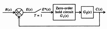
- Using the Nyquist diagram, determine if the system is stable when K = 1.
- Check your answer to part (a) using the bilinear transformation.
- 4.23. Repeat Problem 4.22 if

In addition, find the maximum value of K before the system becomes unstable, and the system's response to a unit step input and a unit ramp input.
- 4.24. A feedback control system has a forward transfer function given by
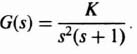
The error channel and feedback channel are sampled at a sampling interval of 1 sec as shown in the block diagram of Figure P4.24. The error and output impulse trains are extrapolated by means of zero-order holding circuits.

- Determine the open-loop z-transfer functions GH(z).
- Using the Nyquist diagram, determine whether the system is stable when K = 1.
- 4.25. Find f(0) and f(∞) in each case:
- 4.26. Consider the open-loop, sampled-data control system illustrated in Figure P4.26. Assume that the sampling rate T is 1 sec and that the input r(t) is a unit pulse lasting for 5 sec. Using z-transform theory, determine the following:
- The z transform of the input, R(z).
- The z transform of the output, C(z).
- The value of c*(t).
- Compute and sketch the value of c(t) using the advanced z transform. Assume that Δ = 0.25, 0.5, and 0.75.
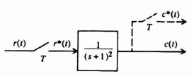
- 4.27. Using the bilinear transformation, determine the stability of sampled-data control systems whose characteristic equations are given by
- z2 + 1.5z − 1 = 0.
- z2 − z + 0.25 = 0.
- z3 − 3z2 + 2.25z − 0.5 = 0.
- 4.28. Repeat Problem 4.27 using the Schur–Cohn stability criterion.
- 4.29. The z transform of a system's response is given by

- Determine the resulting response given by the final-value theorem.
- Find the value of c(k) by taking the inverse transform of C(z) using partial-fraction expansion and a table of z transforms.
- Do your answers to parts (a) and (b) agree?
- 4.30. Determine the maximum value of gain K that can be designed into the sampled-data control systems illustrated in Figure P4.30 before the system becomes unstable. Assume that the sampling period is 1 sec.
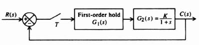
- 4.31. Consider the digital control system in Figure P4.31.
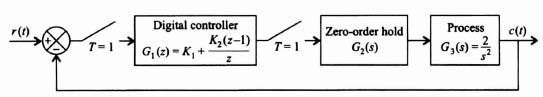
- Determine the characteristic equation for this system.
- It is desired to have two of the roots of the characteristic equation located at z = 0.4 and z = 0.4. Determine the values of K, and K2 to achieve this.
- Determine the location of the third root.
- 4.32. It is desired to design a discrete compensation network for the sampled-data control system illustrated in Figure P4.32 using the Bode-diagram method. The process to be controlled has the following transfer function

and contains a zero-order hold. Assume that the sampling rate of the control system is 0.5 sec.

- 4.33. Repeat the sampled-data problem analyzed in Figure 4.31 of Section 4.9, with the sampling rate increased from 0.26 sec to 0.056 sec. What effect does the faster sampling rate have on the resulting system? Design the compensated system for a gain crossover frequency of 1 rad/sec and a minimum phase margin of 25°.
- 4.34. Consider the digital control system in Figure P4.34.

- Determine the open-loop transfer function, G1G2(z).
- Determine the closed-loop transfer function, C(z)/R(z).
- Determine the characteristic equation of this system.
- Determine the location of the roots of the characteristic equation.
- Is this system stable?
- 4.35. Repeat the analysis of the digital control system illustrated in Figure 4.31 with the sampling time decreased to 0.1 sec from 0.26 sec. Determine the following:
- GH(z)
- GH(ν)
- From the Bode diagram, determine the gain crossover frequency, the phase margin, and the gain margin. Is the system stable or unstable?
- 4.36. The block diagram of a sampled-data control system is illustrated in Figure P4.36. Assume that the sampling rate is 1 sec.
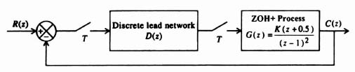
- Assuming that D(z) = 1, sketch the root locus of this system as a function of K. Label all pertinent points. Is the system stable or unstable?
- Design a discrete lead network D(z), so that the dominant poles are at ζ = 0.7 and θ = ±36° (the angle made by the radial lines shown emanating from the origin) in Figure 4.40.
- Plot the closed-loop response to a unit step input for the compensated system. How does the resulting overshoot compare to that predicted for a ζ = 0.7?
- 4.37. It is desired to compensate a sampled-data control system using Ragazzini's method. Assume that it is desired to respond perfectly to a ramp, and that a minimal prototype system is desired. For the system shown in Figure P4.37, assume that the data extrapolator is a zero-order hold, the sampling rate is 1 sec, and G2(s) is given by

- Applying Ragazzini's method, design D(z).
- Determine and sketch the response to a unit step input.
- Determine and sketch the response to a unit ramp input.
- 4.38. Illustrate how the response of the problem analyzed in Problem 4.37 can be softened by the addition of a staleness factor term where the staleness factor C is given by
- C = 0.2.
- C = 0.8.
- 4.39. Repeat Problem 4.36 if the transfer function of the process is given by
- 4.40. Repeat Problem 4.32 if the transfer function of the process is given by

- 4.41. Numerical integration can be approximated by summing rectangular areas under a continuous function, y(t), as shown in Figure P4.41.
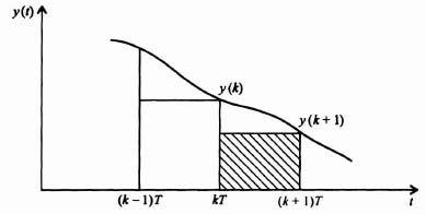
- Defining the integral of y(t) as x(t), write the difference equation relating x[(k + 1)], x(k), and y[(k + 1)] for this method.
- Determine the transfer function for this rule of numerical integration, X(z)/Y(z).
- 4.42. Numerical integration can be approximated by summing trapezoidal areas under a continuous function y(t) as shown in Figure P4.42.
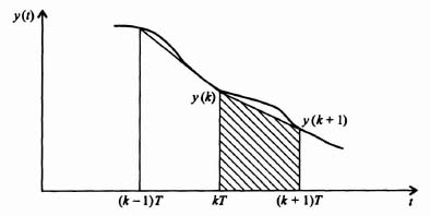
- Defining the integral of y(t) as x(t), write the difference equation relating x(k + 1), x(k), and y(k + 1) for this method.
- Determine the transfer function for this rule of numerical integration, X(z)/Y(z).
- 4.43. A continuous-type phase-lead network, used to compensate a continuous control system, is given by the following transfer function:

It produces a phase-lead of 19.33° at a critical frequency of 0.4 rad/sec.
- Determine the corresponding digitized phase-lead network assuming that the sampling time is 1 sec, and we wish to match the gains at dc.
- Is the digitized phase-lead network stable?
- Compare the phase lead of the digitized phase-lead network with that of the continuous-type phase-lead network at the critical frequency of 0.4 rad/sec.
- 4.44. The digital control system shown in Figure P4.44 contains a process containing a double integration. Assume that the sampling time T is
 sec.
sec.
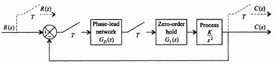
- Determine the z transform of the zero-order hold and the double integration. Assume that the compensating phase-lead network has a gain of one in this part.
- Plot the root locus for this control system. Determine all pertinent points of the root locus including points of breakaway and break-in along the real axis. What does the root locus indicate regarding the stability of this control system?
- Compensate this control system by the addition of a phase lead network, GD(s), so that the control system is conditionally stable.
- Draw the root locus for the compensated control system and indicate all pertinent points of the root locus. Determine the maximum value of K where the root locus intersects the unit circle using the modified Routh–Hurwitz criterion.
- For a desired damping ratio of 0.45, determine the value of K which will achieve this damping ratio.
- Determine the response of the compensated control system with the value of K found in part (e) to a unit step input. What is the maximum percent overshoot to the unit step input? What damping ratio does this maximum percent overshoot correspond to? Does this damping ratio agree with the desired damping ratio of 0.45?
- What would happen if noise entered this digital control system at the input to the process?


REFERENCES
1. J. J. Craig, Introduction to Robotics. Addison-Wesley, Reading, MA, 1986.
2. G. F. Franklin, J. D. Powell, and M. L. Workman, Digital Control of Dynamic Systems, 3rd ed. Addison-Wesley, Reading, MA, 1994.
3. K. Ogata, Discrete-Time Control Systems. Prentice-Hall, Englewood Cliffs, NJ, 1987.
4. C. H. Houpis and G. B. Lamont, Digital Control Systems Theory. Hardware. Software. McGraw-Hill, New York, 1985.
5. C. L. Phillips and H. T. Nagle, Jr., Digital Control System Analysis and Design. Prentice-Hall, Englewood Cliffs, NJ, 1984.
6. C. Shannon, “The philosophy of pulse code modulation.” Proc. IRE 36(11), 1324–1331 (1948).
7. J. R. Ragazzini and G. F. Franklin, Sampled-Data Control Systems. McGraw-Hill, New York, 1958.
8. R. L. Oldenbourg and R. Sartorious, The Dynamics of Automatic Control, Chapter 5. American Society of Mechanical Engineers, New York, 1948.
9. E. I. Jury, “A simplified stability criterion for linear discrete systems.” Proc. IRE 50, 1493 (1962).
10. E. I. Jury and J. Blanchard, “A stability test for linear discrete systems in tabular form. Proc. IRE 49, 1947 (1961).
11. E. I. Jury, Theory and Application of the z-Transform Method. Wiley, New York, 1964.
12. B. C. Kuo, Analysis and Synthesis of Sampled-Data Control Systems. Prentice-Hall, Englewood Cliffs, NJ, 1963.
13. MATLAB™ for MS-DOS Personal Computers User's Guide, Control System Toolbox. MathWorks, Inc., Natick, MA 1997.
14. J. E. Bertram, “Factors in the design of digital controllers for sampled-data feedback control systems.” Trans. Am. Inst. Electr. Eng., Pap. 56–209 (1956).