ANSWERS TO SELECTED PROBLEMS

CHAPTER 1

1. 1.4.
2. 1.6.
   1. Crossover frequency = 4.483 rad/sec, phase margin = 32.44°, gain margin = 8.657dB.
   2. K = 9.9
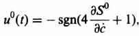
   3. Crossover frequency = 13.61 rad/sec, phase margin = −30.62°, gain margin = −11.26 dB.

CHAPTER 2

1. 2.1.
   1. The electrical network illustrated in Table 2.4^‡, items 3, with

      

      and cascaded with an amplifier whose gain is 4.6 will satisfy the specifications

   2. The electrical network illustrated in Table 2.4^‡, item 4, with

      

      and cascaded with an amplifier whose gain is 4.6 will satisfy the specifications.

   3. The electrical network illustrated in Table 2.4^‡, item 5, with

      

      will satisfy the specifications.

2. 2.2.
   1. ζ = 0.5; ω_n = 4 rad/sec; maximum percent overshoot = 16.4%; steady-state error = 0.25.
   2. b = 0.15.
   3. Maximum percent overshoot = 1.5%; steady-state error = 0.4.
   4. Add a high-pass filter in cascade with the tachometer as illustrated in Figure 2.15.
3. 2.5.
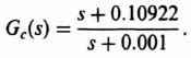
   1. G_c(s) = 1 + 0.382s.
   2. b = 0.382.
4. 2.7.
5. 2.8.
   1. 

      the attenuation of 1/178.6 due to the two lead networks is assumed to be compensated for by increasing the gain of the amplifier by 178.6. The result is a phase margin of 46.9° at a gain crossover frequency of 6.4 rad/sec, and a gain margin of 32.8 dB at a phase crossover frequency of 68 rad/sec.

   2. 
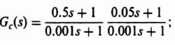
6. 2.11. A phase-lead network whose transfer function is

   

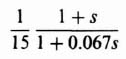
   The result is a phase margin of 44.8° at a gain crossover frequency of 2.35 rad/sec, and a gain margin of 11.2 dB at a phase crossover frequency of 11.2 rad/sec, assuming that the attenuation of the phase-lead network of is compensated for by boosting the gain of the amplifier by a factor of 15. Therefore, this phase-lead network achieves the design specification of a minimum phase margin of 60°.

7. 2.12. Same answer as for Problem 2.11.
8. 2.14. Two cascaded phase-lead networks are required to meet these specifications. Their transfer function, together with the gain given of 99, is given by

   

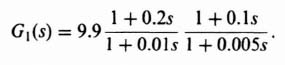
   The constant attenuation of 400 due to the characteristics of these two phase-lead networks must be made up by an amplification increase of 400. The resulting phase margin is 46.09° at a gain crossover frequency of 55.58 rad/sec.

9. 2.15.
   1. ω_c = 3 rad/sec.
   2. 

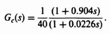
   It is assumed that the attenuation of 1/40 is compensated for by increasing the gain of the amplifier. This phase-lead network provides a phase margin of 71.86° at a new gain crossover frequency of 8.078 radians/second.

10. 2.20.
    1. 

       The constant attenuation of 1.08 due to the characteristics of this phase-lead network must be made up by an amplification increase of 1.08.

    2. For part (a), ω_p = 2.375 rad/sec, M_p = 1.154 dB.
11. 2.21.
    1. 

       The attenuation due to the phase-lead network is assumed to be compensated for by increasing the gain of the amplifiers.

    2. For the phase-lead network, M_p = 0.7513 dB, ω_p = 3.864 rad/sec.
12. 2.22.
    1. b = 0.25.
    2. e_ss = 0.3024.
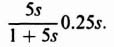
    3. The transfer function of the rate feedback path is given by

       

    4. e_ss = 0.0524.
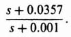
13. 2.23. The phase-lag network is given by

    

14. 2.28. K = 4.22.
15. 2.38. K = 2.226.
16. 2.40.
    1. K = 129.3.
    2. M_p = 4.24 dB; ω_p = 10.67 rad/sec.
17. 2.41 K = 25.57.

CHAPTER 3

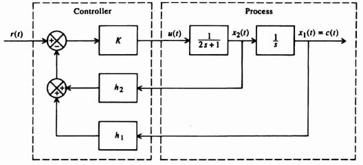
1. 3.2.
   1. 
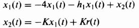
   2. s² + 4s + h₁s + K = 0.
   3. 
   4. 
   5. The proportional plus integral controller configuration of part (d) produces a zero term which would aid in the stability compensation of this control system. The controller configuration of part (a) does not have this feature, and it would be more difficult to stabilize.
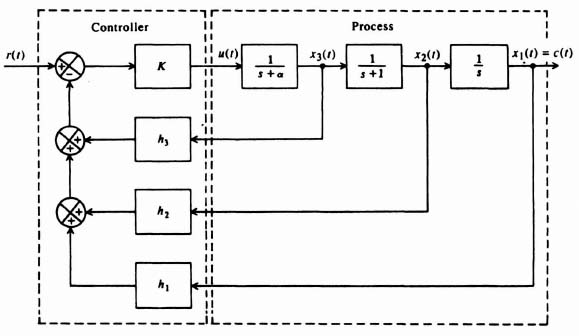
2. 3.6. The synthesized system is illustrated in Figure A3.6, where

   

   A root locus analysis indicates that a good choice of α is approximately 2.5. Therefore, h₃ becomes

   

   Figure A3.6

3. 3.8.
   1. Yes.
   2. see Figure A3.8.
   3. K = 20,000.

      h₁ = 1,

      h₂ = 0.00995.

   4. Root locus shows that the system is stable.
4. 3.10.
   1. 

      System is not controllable.

   2. 

      System is observable.

5. 3.11.
   1. 

      System is controllable.

   2. 

      System is unobservable.

6. 3.13.

   

   Figure A3.8

7. 3.15.
8. 3.17.
9. 3.20.

CHAPTER 4

1. 4.3.
2. 4.5.
3. 4.7.
   1. e(k) = 2(1 − 0.5^k), k ≥ 0.
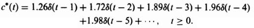
   2. e(k) = δ(k − 1) + 1.5δ(k − 2) + 1.75δ(k − 3) + 1.875δ(k − 4) +…, k = 0, 1, 2,….
4. 4.8.
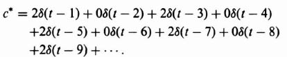
   1. R(z) = 0.5z⁻¹ + z⁻² + 0.5z⁻³.
   2. 
   3. 
   4. 
5. 4.10. G(z) = (z/(z − e^−T)) − (1/(z − e^P − 2T)).
6. 4.12. c(k) = 2^k − k ≥ 0.
7. 4.14.
8. 4.18.
   1. 
   2. 
   3. 
   4. c(0) = 0.
   5. c(∞) = 2.
9. 4.20.
   1. G(z) = 0.5(z + 1)/z(z − 1).
   2. 
   3. 
10. 4.22. The system is unstable with two roots in the right half-plane.
11. 4.25. The final-value theorem cannot be used in all three parts because the function is not analytic in the right half-plane. f(0) = 0 in all three parts.
12. 4.28.
    1. Unstable with one root outside the unit circle of z-plane.
    2. Stable.
    3. Unstable with two roots outside unit circle of z-plane.
13. 4.29.
    1. c(∞) = 4
    2. c(k) = 4[1 − k(0.5)^k − (0.5)^k].

       Therefore, c(∞) = 4.

    3. Yes.
14. 4.30. K must be less than 2.17.
15. 4.41.
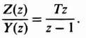
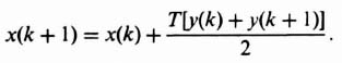
    1. x[(k + 1)] = x(k) + Ty(k + 1).
    2. 
16. 4.42.
    1. 
    2. 

CHAPTER 5

1. 5.1.
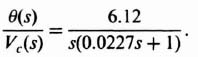
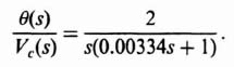
   1. Transfer function of the motor with one straight line tangent to the exact characteristics at 1000 rev/min is

      

      Transfer function of the motor with one straight line going through the two endpoints is

      

   2. Transfer function of the motor with one straight line tangent to the characteristics at 250 rev/min is

      

      Transfer function of the motor with one straight line tangent to the characteristics at 1750 rev/min is

      

2. 5.2.
3. 5.3.
4. 5.4.
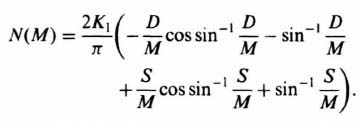
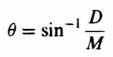
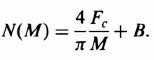
5. 5.7. N = 0 for M ≤ D

   

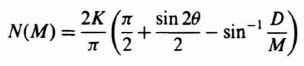
   where

   

6. 5.8.
7. 5.17.
   1. See Figure A5.17.

      

      Figure A5.17

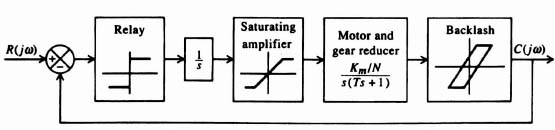
   2. For the linear elements, their transfer functions can be combined into a transfer function, G(s). For the nonlinear elements, a new describing function which represents the combined nonlinear effects of saturation, the relay, and backlash would have to be derived. Then, −1/N and G(jω) could be plotted on the gain-phase diagram to determine the presence of an oscillation.
8. 5.18. A stable limit cycle occurs at D/M = 0.999 and ω = 0.0707 rad/sec.
9. 5.19. A limit cycle does not exist.
10. 5.21. System is stable and exhibits no limit cycle.
11. 5.22. Unstable limit cycle occurs at M/D = 0.045 and ω = 15.6 rad/sec.
12. 5.23. System is stable and exhibits no limit cycle.
13. 5.25. System does not exhibit the existence of any limit cycles.
14. 5.26.
    1. Limit cycles occur at D/M = 0.8319, ω = 0.3846 rad/sec; D/M = 0.2533, ω = 1.033 rad/sec,

       The former limit cycle is unstable, the latter is stable.

    2. K = 2.75.
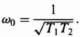
    3. αT = 0.9 sec, T = 0.4 sec (assume increase in original gain by a factor of ).
    4. b = 0.32.
15. 5.30. A stable limit cycle exists at ω = 30 rad/sec and D/M = 0.62. An unstable limit cycle exists at ω = 3 rad/sec and D/M = 0.92.
16. 5.31. The describing-function analysis of the gain-phase diagram indicates that limit cycles do not exist for this system if the nonlinearity corresponds to Coulomb friction.
17. 5.32. System does not exhibit the existence of any limit cycles.
18. 5.35.
    1. The phase trajectory is a circle through the point 1, 0 and whose center is the origin.
    2. The system is unstable, since no viscous damping is present.
19. 5.43.
    1. 
    2. 
    3. 
    4. 
20. 5.44.
    1. The isocline equation is given by

       

       where

       

    2. The isocline equation is given by

       

       where

       

    3. The isocline equation is given by

       

       where

       

    4. The isocline equation is given by

       

       where

       

21. 5.49. Defining

    

    and

    

    the isocline equation is given by

    

    where

    

    and

    

22. 5.51.
    1. Asymptotically stable.
    2. Unstable.
    3. Asymptotically stable for

       

23. 5.57. Popov condition satisfied if 0 < K 5.5.
24. 5.59. Popov condition satisfied if 0 < K 89.14.
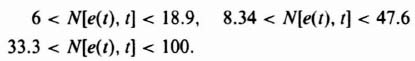
25. 5.63. Possible Popov sectors which result in stable systems are given by the following conditions:

    

CHAPTER 6

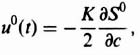
1. 6.3. The optimal input is given by

   

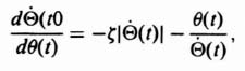
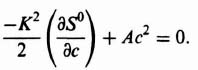
   and the nonlinear partial differential equation to be solved for S⁰ is given by

   

2. 6.4.

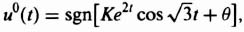
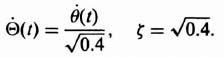
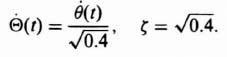
   where K and θ are determined from the boundary conditions of the system.

3. 6.7.
   1. 
   2. u⁰(t) = sgn(4p₂ − 1).
   3. Both results are equal because .
4. 6.13. The optimal control policy is given by

   

   and the nonlinear partial differential equation to be solved for S⁰ is given by

   

5. 6.14. u⁰(t) = Usgn[Ke^t/2 sin(0.866t + θ), where K and θ are determined from the boundary conditions of the system.
6. 6.15. u⁰(t) = Usgn[Ke^t sin(1.732t + θ), where K and θ are determined from the boundary conditions of the system.
7. 6.16. u⁰(t) = Usgn[K₁e^t + K₂te^t), where K₁, K₂, and θ are determined from the boundary conditions of the system.

CHAPTER 7

1. 7.3.
   1. (a) Pertinent characteristics of the root locus are
      1. (b) Root locus occurs along the real axis between the origin and −2.
      2. (c) The asymptotes intersect the real axis at −1 with angles of ±90°.
      3. The point of breakaway from the real axis occurs at −1.
   2. K = 2.
   3. 
   4. (d),(e) Maximum percent overshoot of the third-order compensated system is 11%, which compares with the maximum percent overshoot of a second-order system which has a damping ratio of 0.707 or 4.3%.
2. 7.5.
   1. Root-locus plot of Figure A7.5a indicates that K = 2.927.

      

      Figure A7.5

   2. 
   3. Root-locus plot of Figure A7.5b indicates that

      

3. 7.7.
   1. 

      This corresponds to an overdamped response.

   2. 

      This corresponds to a critically damped system.

   3. 

      This corresponds to an oscillation having a stable amplitude of 2 (peak-to-peak) centered about 1.

   4. 

      This corresponds to a growing oscillation.