APPENDIX B

CHARACTERISTIC RESPONSES OF SECOND-ORDER CONTROL SYSTEMS

The purpose of this appendix is to describe the transient response of a typical feedback control system which is referred to many times in this book. We consider a very common configuration in which a two-phase ac servomotor is enclosed by a simple unity feedback loop. Figure 4.1 illustrates the block diagram of this second-order system. For purposes of simplicity, the gain of the amplifier driving the motor is assumed to be unity.

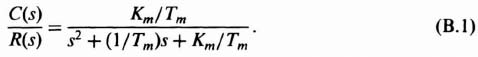
The closed-loop transfer function of this system is given by

By defining the undamped natural frequency ω_n and the dimensionless damping ratio ζ as

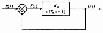
Figure B.1 Second-order feedback system containing a two-phase ac servomotor.

Eq. (B.1) can be rewritten as

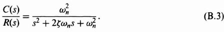
The parameters ω_n and ζ are very important for characterizing a system's response. Note from Eq. (B.3) that ω_n turns out to be the radian frequency of oscillation when ζ = 0. As ζ increases from 0, the oscillation decays exponentially and becomes more damped. When ζ 1, an oscillation does not occur.

We assume that the initial conditions are zero and the input is a unit step. Therefore, R(s) = 1/s, and the Laplace transform of the output can be written as

Factoring the denominator, we obtain

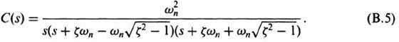
The exact solution for the output in the time domain is dependent on the value of ζ. When ζ 1, the second-order system has poles which lie along the negative real axis of the complex plane. When ζ < 1, however, a pair of complex-conjugate poles result. We shall determine the output response to a step input for the three cases: where the damping ratio equals unity, is greater than unity, and is less than unity.

Case A. Damping Ratio Equals Unity

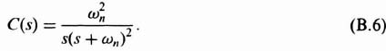
When ζ = 1, Eq. (B.5) reduces to

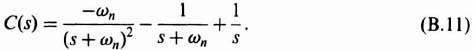
The time-domain response will next be obtained. The partial-fraction expansion of Eq. (B.6) is given by

We find that

Substituting these constants into Eq. (B.7), we obtain

The time-domain response of the output, c(t), may be obtained by utilizing a table of Laplace transforms:

Figure B.2a illustrates the output response together with the unit step input. Notice that the output response exhibits no overshoots when ζ = 1. The response is described as being critically damped.

Case B. Damping Ratio Greater than Unity

When ζ > 1, the time-domain response can be obtained quite simply from its partial fraction expansion. This can be expressed as

where are positive real numbers.

The constants K₁, K₂, and K₃ can be evaluated quite simply by the methods of partial fraction expansion. Their values are

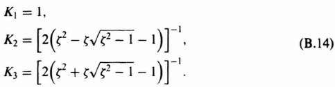
Therefore Eq. (B.13) can be written as

The time-domain response of the output, c(t), may be obtained by utilizing a table of Laplace transforms. It can be expressed as

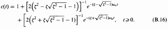
Figure B.2b illustrates the output response together with the unit step input. Notice that when ζ > 1, the output response exhibits no overshoots and takes longer to reach its final value than when ζ = 1. This response is described as being overdamped.

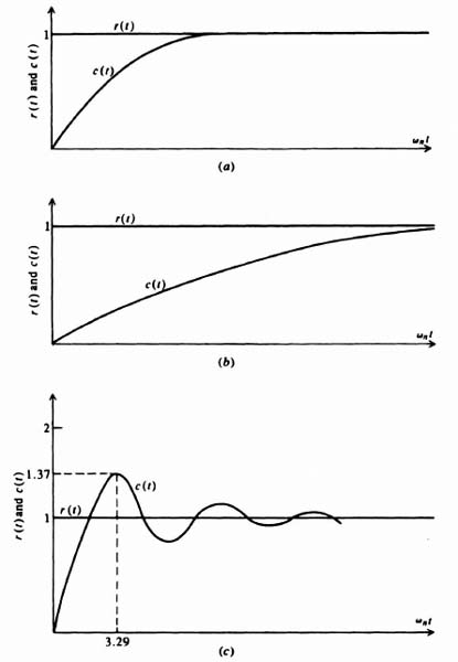
Figure B.2 (a) Input and output response for a critically damped second-order system; (b) input and output response for an overdamped second-order system; (e) input and output response for an under-damped second-order system

Case C. Damping Ratio Less than Unity

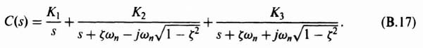
When ζ < 1, the time-domain response can be obained in an analogous manner. The solution is slightly more complex, however, because we now have a pair of complex-conjugate poles. The partial fraction expansion of Eq. (B.5) can be written as

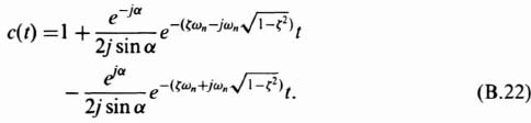
The constants K₁, K₂, and K₃ can be evaluated in an analogous manner by the method of partial fraction expansion, but the algebra becomes a little complicated. In order to simplify this situation somewhat, use is made of the relationship between the location of the complex-conjugate poles in the complex plane and the damping ratio ζ. The geometry of the configuration is illustrated in Figure B.3. Notice that the distance from the origin to either pole equals ω_n. In addition, the angle a has the following trigonometric properties:

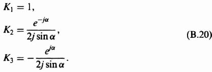
Utilizing the relations given by Eqs. (B.18) and (B.19), the constants K₁, K₂, and K₃ can be expressed as

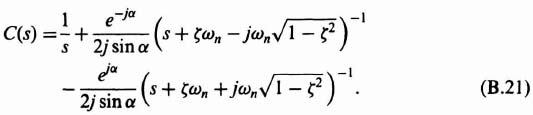
Therefore Eq. (B.17) can be written as

The time-domain response of the output, c(t), may be obtained by utilizing a table of Laplace transforms. It can be expressed as

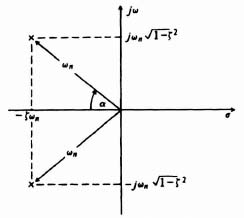
Figure B.3 Location of the complex-conjugate poles in the complex plane.

This can be simplified to

or

Figure B.2c illustrates the output response for a value of ζ which has a value of 0.3, together with the unit step input. Notice that the output response exhibits several overshoots and undershoots before finally settling out. This response, which is characteristic of an exponentially damped sinusoid, is described as being underdamped.

Examination of Eq. (B.24) indicates that the term in the exponent, ζω, multiplies t and it controls the exponential decay or rise of the unit step response, c(t). Therefore, ζω_n determines the “damping” of the system and it is defined as the damping factor of the system. Note that the inverse of ζω_n is proportional to the time constant of the system.

Observe from Eq. (8.12) that when the system is critically damped and ζ = 1, the damping factor equals ω_n. Therefore, we view ζ as the damping ratio which is defined as follows:

The time to the first overshoot and the value of the first overshoot are two interesting identifying characteristics for this type of response. We shall next derive these values in terms of the undamped natural frequency ω_n and the damping ratio ζ.

Equation (B.24) indicates that the damped natural radian frequency of oscillation of the system, ω_m, is

The damped natural cyclic frequency of oscillation of the system, f_m, is

The period of oscillation of the underdamped system, t_m, is

The time at which the peak overshoot occurs, t_p, is found by differentiating c(t), from Eq. (B.24), with respect to time and setting the derivative equal to zero:

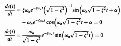
This derivative is zero when

The peak overshoot occurs at the first value after zero, provided there are zero initial conditions. Therefore, the time to the first peak, t_p and ω_nt_p are given by

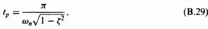
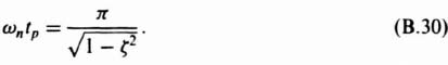
For the case illustrated in Figure B.2c, where ζ = 0.3, the time to the first overshoot is 3.29/ω_n.

Substituting Eq. (B.30) into Eq. (B.24) yields the value for the maximum instantaneous value of the output, c(t):

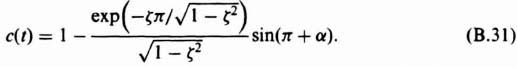
This can be simplified by substituting

Therefore,

This is usually expressed as a percentage of the input. Therefore, for a unit step input,

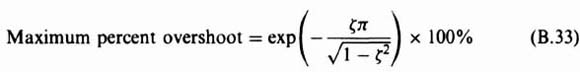
For the case illustrated in Figure B.2, where ζ = 0.3, the maximum percent overshoot is 37%.

The second-order system is a very common and popular one. In order for the reader to become more familiar with its typical characteristic responses, Figure B.4 is shown to illustrate the resulting transient responses and percent maximum overshoots, rexpectively, for several values of damping ratios.

Figure B.4 Transient response curves of a second-order system to a unit step input.