2

LINEAR CONTROL-SYSTEM COMPENSATION AND DESIGN

2.1. INTRODUCTION

After the stability of a feedback control system has been analyzed, by using any of the tools presented in Chapter 1, it will often be found that system performance is not satisfactory and needs to be modified. It is necessary to ensure that the open-loop gain is adequate for accuracy, and that the transient response is desirable for the particular application. In order for the system to meet the requirements of stability, accuracy, and transient response, certain types of equipment must be added to the basic feedback control system. We use the term design to encompass the entire process of basic system modification in order to meet the specifications of stability, accuracy, and transient response. The term stabilization is usually used to indicate the process of achieving the requirements of stability alone; the term compensation is usually used to indicate the process of increasing accuracy and speeding up the response.

There are several commonly used configurations for compensating (or stabilizing) a control system. The compensating (or stabilizing) device may be inserted into the system either in cascade with the forward portion of the loop (cascade compensation) as shown in Figure 2.1, or as part of a minor feedback loop (feedback compensation) as shown in Figure 2.2 [1,2]. The cascade-compensation technique is usually concerned with the addition of phase-lag, phase-lead, and phase-lag–lead passive networks. The feedback-compensation technique is primarily concerned with the addition of rate or acceleration feedback. The type of compensation chosen usually depends on the nonlinearities and the location of the noises in the loop, and economic considerations.

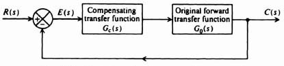
Figure 2.1 Illustration of series or cascade compensation.

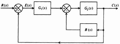
Figure 2.2 Illustration of minor-loop feedback compensation.

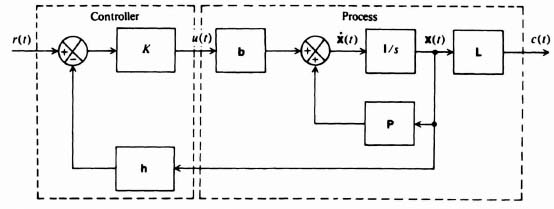
Figure 2.3 Illustration of linear-state-variable-feedback compensation.

Linear-state-variable-feedback compensation, illustrated in Figure 2.3, consists of feeding back the state variables through constant real gains.

Linear-state-variable feedback requires that all state variables be fed back to the controller. For very high-order control systems, it requires a larger number of transducers to sense the state variables for feedback. Therefore, practical applications of this technique can be very costly or impractical. In addition, some state variables may not be directly accessible (e.g., nuclear power plant processes), and this can limit this technique's application even in low-order control systems. For cases where some state variables may not be directly accessible, we use an estimator to estimate the state variables from measurements made of the accessible variables. Figure 2.4 illustrates an estimator system for a regulator system where the reference input r(t), equals zero.

The compensation techniques illustrated in Figures 2.1 through 2.4 all have only one degree of freedom because there is only one controller in each system, even though the controller can have more than one parameter which can be varied. These one-degree-of-freedom controllers have the major disadvantage that the performance criteria which can be achieved is limited. For example, if a control system is designed to have a desired stability, then it may have poor sensitivity to parameter variations. Let us, therefore, next consider compensation techniques which have two degrees of freedom.

Figure 2.4 Illustration of an estimator system for a regulator system (where the reference input r(t) = 0).

Figure 2.5 illustrates the series-feedback compensation technique in which a series controller and a feedback controller are used. This technique is denoted as having two degrees of freedom compensation because it has two controllers, the series controller G_c(s) and the feedback controller B(s).

Figure 2.6 illustrates forward compensation in which the feedforward controller G_c1(s) is in series with the closed-loop control system which also has a controller G_c2(s) in the forward part of the control system. Because the controller G_c1(s) is not within the feedback loop of the control system, it does not affect the characteristic equation roots of the original control system. Therefore, the poles and zeros of G_c1(s) can be designed to cancel (or add) to the poles and zeros of the closed-loop transfer function. This technique is also referred to as having two degrees of freedom compensation because it has two controllers, the series controller G_c1(s) and the forward-loop controller G_c2(s).

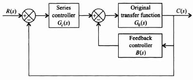
Figure 2.5 Series-feedback compensation technique illustrating two degrees of freedom.

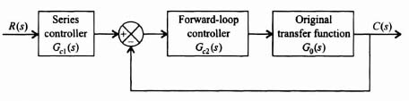
Figure 2.6 Forward compensation with series compensation illustrating two degrees of freedom.

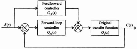
Figure 2.7 Feedforward compensation illustrating two degrees of freedom.

Figure 2.7 illustrates another form of two degrees of freedom compensation system which uses a feedforward controller, G_c1(s), which is placed in parallel with the forward path which contains the controller G_c2(s).

This chapter focuses attention on the tools presented in Chapter 1 which are of practical and useful interest to the control engineer. We will focus our attention on the application of the techniques to those particular design problems they are most suited to solve. Chapter 3 presents modern control-system design techniques using state-space techniques, Ackermann's formula for pole placement, estimation, robust control, and the H^∞ method for sensitivity reduction. Chapter 6 discusses the design of linear feedback control systems from the point of view of modern optimal control theory. Additional linear design problems are presented in Chapter 7 where actual case studies are outlined.

2.2. CASCADE-COMPENSATION TECHNIQUES

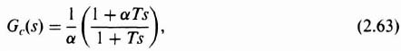
Let us consider the system of Figure 2.1 as our basic starting point in order to analyze the effect of cascade compensation. The compensating transfer function G_c(s) is designed in order to provide additional phase lag, phase lead, or a combination of both at certain frequencies, in order to achieve certain specifications regarding stability and accuracy. We will illustrate and derive the transfer functions for representative compensating passive networks [1–6].

A phase-lag network is a device that shifts the phase of the control signal in order that the phase of the output lags the phase of the input over a certain range of frequencies. An electrical network performing this function was illustrated in Table 2.4^‡ as item 4. Its transfer function was

This can be written in the following more useful form:

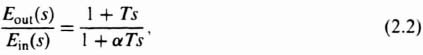
Figure 2.8 A complex-plane plot for a phase-lag network.

where

Observe that αT > T. A complex-plane plot of this network as a function of frequency is shown in Figure 2.8. Notice that the output voltage lags the input in phase angle for all positive frequencies. In addition, observe that the magnitude of E_out(jω)/E_in(jω) decreases from unity at ω = 0 to 1/α at ω = ∞. The Bode diagram for the phase-lag network is illustrated in Figure 2.9. The frequency at which the maximum phase lag occurs, ω_max, and the maximum phase lag, φ_max, can be easily derived. The results are

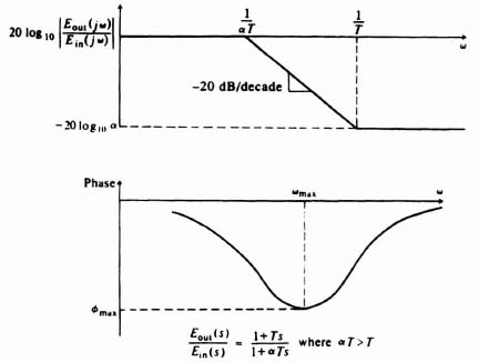
Figure 2.9 Bode diagram of a phase-lag network.

and

Values of φ_max for certain values of α, which are useful for design purposes, are listed in Table 2.1.

A phase-lead network is a network which shifts the phase of the control signal in order that the phase of the output leads the phase of the input at certain frequencies. An electrical network performing this function was illustrated in Table 2.4^‡ as item 3. Its transfer function was as follows:

This can be written in the following more useful form:

where

Observe that αT > T. A complex-plane plot of this network as a function of frequency is shown in Figure 2.10. Notice that the output voltage leads the input in phase angle for all positive frequencies. In addition, notice that the magnitude of E_out(jω)/E_in(jω) increases from 1/α at ω = 0 to unity at ω = ∞. The Bode diagram for the phase-lead network is illustrated in Figure 2.11. The corresponding values of ω_max and φ_max for the phase-lead network are

and

Table 2.1. φ_max as a Function of α

α	φmax (degress)
1	0
2	−19.4
3	−36.9
4	−51.0
5	−55.0

^‡Throughout the book, this symbol is used to refer to material in the companion volume. Modern Control System Theory and Design, Second Edition.

Figure 2.10 A complex-plane plot for a phase-lead network.

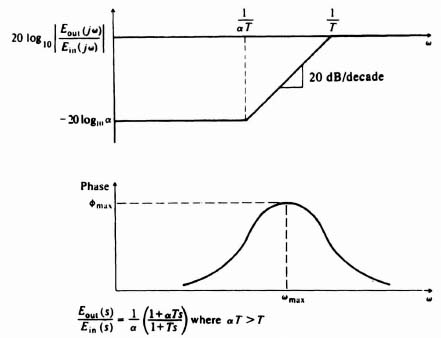
Figure 2.11 Bode diagram of a phase-lead network.

The values shown in Table 2.1 are also true for the phase-lead case except for the sign. An important practical point to emphasize is that the control engineer would not in practice use any ratio of α > 10 because the lead network acts as an attenuation, which must be made up for somewhere in the feedback control system, with an amplification whose ratio is α.

A phase-lag–lead network is a network that shifts the phase of a control signal in order that the phase of the output lags at low frequencies and leads at high frequencies relative to the input. An electrical network performing this function was illustrated in Table 2.4^‡ as item 5. Its transfer function was as follows:

Defining

we can rewrite Eq. (2.9) as

A complex-plane plot of this network as a function of frequency is shown in Figure 2.12. Notice that the output voltage lags the input in phase angle for low frequencies and leads in phase angle for high frequencies. In addition, notice that the magnitude of E_out(jω)/E_m(jω) decreases for intermediate frequencies and increases to unity as ω approaches 0 and ∞. A corresponding Bode diagram for the phase-lag–lead network is illustrated in Figure 2.13.

Figure 2.12 A complex-plane plot for a phase-lag–lead network.

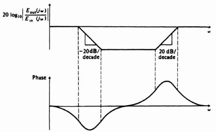
Figure 2.13 Bode diagram of a phase-lag–lead network.

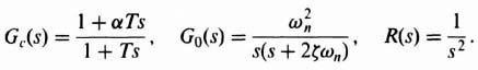
The stabilizing effect of cascaded, phase-shifting networks can easily be demonstrated for a simple second-order system. For example, let us consider the configuration illustrated in Figure 2.1, where the original forward transfer function G₀(s), is given by

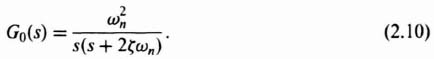
If this system were uncompensated [G_c(s) = 1], then the transfer function G₀(s) would result in the familiar second-order system response which is discussed at great length in Appendix B. The resulting damping ratio of the system would be given by ζ and its undamped natural frequency by ω_n. Let us now assume that we add a lead network to this system whose transfer function is given by

It is assumed that the attenuation factor of 1/α is compensated for with an amplification increase of α, and the system will maintain the same static error. Let us consider the case where T αT and, therefore, G_c(s) can be approximated by a zero factor (proportional plus derivative control):

Another way of looking at this approximation is the viewpoint of adding a rate feedback loop. In the following section, it is shown in Figure 2.14α that the addition of rate feedback bs in parallel with unity position feedback is equivalent to adding the pure zero factor term (1 + bs) to the open-loop transfer function, G(s)H(s). Therefore, the approximation in Eq. (2.12) can be viewed as an approximate representation of a phase-lead network, or the exact representation of the addition of rate feedback in parallel with position feedback to the system. In the following analysis, we will use the terminology of Eq. (2.12), which is based on an approximation to the phase-lead network, although it could just as easily represent exactly the addition of rate feedback in parallel with position feedback.

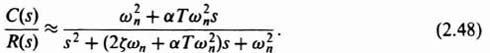
The form of Eq. (2.12) suggests that this lead network (or the addition of rate feedback in parallel with unity position feedback) is equivalent to a proportional plus derivative controller. The resulting system transfer function with the lead network is given by

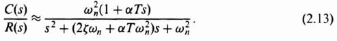
Comparing the denominators of Eqs. (2.13) and (B.3) of Appendix B, we observe that it is still of second order and ω_n remains the same, but ζ is greater due to the increase in the coefficient of s in the denominator. The equivalent damping ratio with G_c(s) can be obtained as follows:

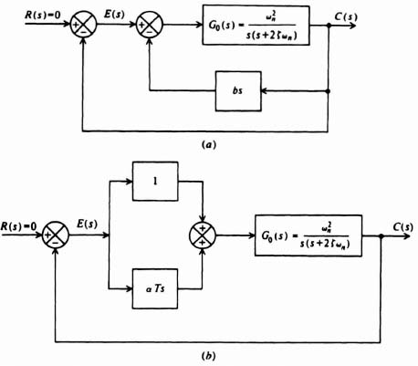
Figure 2.14 The stabilizing effects of the systems illustrated are equivalent. (a) Feedback compensation. (b) Cacade compensation—proportional plus derivative controller

where ζ_eq is an equivalent damping ratio with the addition of a zero factor for compensation. Solving for ζ_eq, we obtain

Therefore, we can conclude that the addition of a zero factor in G_c(s) has increased the damping ratio from ζ to ζ_eq by an amount equal to αTω_n/2. This assumes that T is positive, or the zero of the factor (1 + αTs) is in the left half of the s-plane.

The next question is what is the steady-state error resulting from cascade compensation? To answer this, we must find the steady-state errors resulting from the application of a unit ramp input for the cases of no compensation and compare them with those resulting from cascade compensation. We choose a unit ramp as our input because it is the only input which results in a finite response error for a system with a pole at the origin. The transfer function relating error to input for the system shown in Figure 2.1 is given by

Assuming that

and

we find that

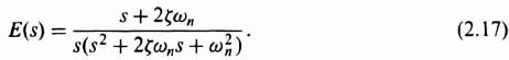
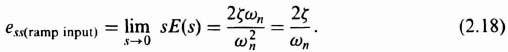
Applying the final-value theorem to Eq. (2.17), we find the steady-state error to be

For the case with cascade compensation, a similar analysis yields the following result:

Therefore,

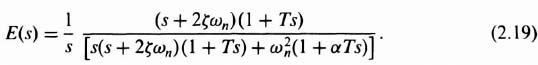
Applying the final-value theorem to Eq. (2.19), the steady-state error is found to be

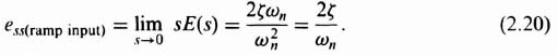
Comparing the results of Eqs. (2.18) and (2.20), we conclude that the addition of the cascade lead network as given by Eq. (2.11) does not increase or decrease the steady-state response error of the system.

It is important to emphasize that the relationships derived in this analysis apply only to the simple system considered. For example, if a zero factor were contained in the numerator of Eq. (2.10), then these relationships are modified (see Problems 2.5 and 2.6).

If we attempt to extend this analysis of a second-order system to the case of phase-lag compensation, the characteristic equation becomes third order and difficult to factor. For example, if G_c(s) were only to represent the pole factor of the phase-lag network, then

In a similar manner, the closed-loop system transfer function can be found to be given by

The factorization of this characteristic equation is not trivial and a similar analysis to that performed for the phase lead-network case is more complex. The root-locus method is an excellent tool which can be used for factorization, and the analysis of this problem for third- and higher-order systems is presented in Sections 1.7 and 2.9.

2.3. MINOR-LOOP FEEDBACK-COMPENSATION TECHNIQUES

Let us consider the general system illustrated in Figure 2.2. The compensating element in this case is the transfer function B(s). In order to have a basis of comparison, we will follow an analysis for minor-loop feedback compensation similar to that performed for the case of phase lead-network cascade compensation.

The minor-loop feedback element B(s) usually represents rate feedback or acceleration feedback. In general, phase-lag, -lead, and/or lag–lead networks may also be cascaded with B(s).

The stabilizing effect of minor-loop feedback compensation can easily be demon-strated for a simple second-order system. We assume that the system illustrated in Figure 2.2 contains simple rate feedback. The specific transfer functions for the system are

The system is redrawn with these transfer functions and shown in Figure 2.14a.

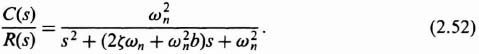
Without any rate feedback, the configuration represents a simple second-order system whose damping ratio is ζ and undamped natural frequency is ω_n. The resulting system transfer function with rate-feedback compensation is given by

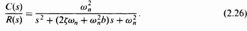
Comparing the denominator of Eq. (2.26) with that of Eq. (8.3), we observe that it is still of second order and ω_n remains the same, but ζ is greater due to the increase in the coefficient of s in the denominator. The equivalent damping ratio with rate feedback added can be obtained by setting the coefficients of the s terms equal to each other, as follows:

where ζ_eq = an equivalent damping ratio with rate feedback added. Solving for ζ_eq we obtain

Therefore, we can conclude that the addition of the minor loop using rate feedback has increased the damping ratio from ζ to ζ_eq by an amount equal to ω_nb/2. This assumes that b is positive (negative feedback).

It is important at this point to compare Eqs. (2.15) and (2.28). Note that they are very similar, and they imply that

The fact that rate feedback behaves as the approximated phase lead network, as defined by Eq. (2.12) (porportional plus derivative controller), can be easily demonstrated from Figure 2.14a and b. Let us assume that there is zero input to both systems, because we are concerned only with the system poles. Clearly, in both cases, there are two negative-feedback paths in parallel around G₀(s). In the cascade-compensation case, the total feedback around G₀(s) is 1 + αTs; in the rate-feedback-compensation case, the total feedback around G₀(s) is 1 + bs. Therefore, the stabilizing effects of αT and b are equivalent. We discuss proportional plus derivative (PD) controllers fully in the next section, 2.4, on proportional-plus-integral-plus-derivative (PID) compensators.

Let us next determine the steady-state error resulting from the use of minor-loop rate-feedback compensation. We assume that the input to this system is a unit ramp in order to have a finite steady-state response error and a basis for comparison. From our discussion of cascade compensation in Section 2.2 we know from Eq. (2.18) that the resulting steady-state error of this system without any compensation (b = 0) is 2ζ/ω_n. For the case of minor-loop rate-feedback compensation, the resulting expression for E(s) is given by

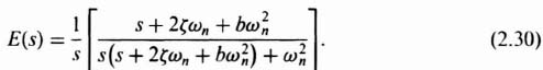
Applying the final-value theorem, the steady-state error is found to be

Therefore, the steady-state response error of the system with minor-loop rate-feedback compensation has increased by a factor of b. This unfavorable result can easily be remedied by placing a high-pass filter in cascade with the rate device. Such a filter would block the steady-state value of the rate output. This technique is illustrated in Figure 2.15.

As in the preceding section, it is important to emphasize that the relationships derived apply only to the simple system considered. Problems 2.5 and 2.6 illustrate how these relationships change if a zero factor is added to the basic system transfer function considered.

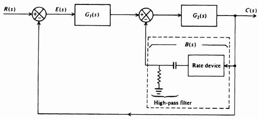
Figure 2.15 Illustration of minor-loop feedback compensation using a rate device in cascade with a high-pass filter

2.4. PROPORTIONAL-PLUS-INTEGRAL-PLUS DERIVATIVE (PID) COMPENSATORS

PID compensators are another form of compensation frequently used in control systems, especially in the industrial process control field. They are very popular in the industrial process control field due to their robust (insensitive) performance over a wide range of operating conditions including plant uncertainty, parameter variation, and external disturbances. Robust control is presented in Section 3.10 of Chapter 3.

Assuming that the input to the PID compensator is e(t) and its output is u(t), the equation defining the operation of the PID compensator is given by:

Figure 2.16 illustrates a block diagram representation of Eq. (2.32). The transfer function of the PID compensator is obtained as follows:

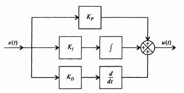
Figure 2.16 PID compensator block-diagram representation of Eq. (2.32).

The resulting transfer function of the PID compensator, G_c(s), is given by

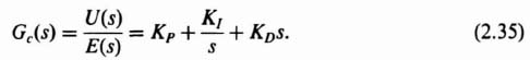
Figure 2.17 illustrates a block diagram representation of Eq. (2.35). Observe from Eqs. (2.32) and (2.35) that the PID compensator provides a proportional term, an integration term, a derivative term, as its name implies.

Very often, only a portion of the very general PID compensator is used. For example, if K_D = 0, then we have

which is denoted as the proportional plus integral, or PI, compensator. If K_I = 0, then we have

which is denoted as the proportional plus derivative, or PD, compensator. This was illustrated previously in Figure 2.14.

To consider the design of a PID compensator, let us reconsider the transfer function of G_c(s) given by Eq. (2.35):

This can be rewritten as

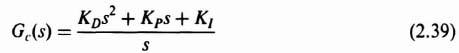
or,

Figure 2.17 PID compensator block diagram representation of Eq. (2.35).

where

Factoring the numerator of Eq. (2.40), and assuming the quadratic factors as two real zeros, we obtain the following:

The very pleasing result of Eq. (2.41) is that the PID compensator results in two zero factors which can be located anywhere in the left-hand of the s-plane, in addition to the pole at the origin. We know from the analysis in Sections 2.2 and 2.3 that a zero factor provides a phase lead and aids in the compensation of a control system. In particular, as illustrated in Figure 2.14b, a PD is equivalent to one zero factor (which the rate feedback compensator also provides and is illustrated in Figure 2.14a). With the complete PID compensator, two zero factors are provided for compensation, in addition to the pole at the origin.

Applications of PI, PD, and PDI compensators are illustrated throughout this book for compensating control systems. These techniques are very useful for compensation of control systems in addition to the phase-lag, phase-lead, and phase-Iag-lead networks illustrated in Section 2.2, and minor-loop rate feedback illustrated in Section 2.3.

2.5. EXAMPLE FOR THEDESIGN OF A SECOND-ORDER CONTROL SYSTEM

In this section we consider the design and resulting performance of the second-order system by means of cascade and minor-loop rate-feedback techniques. This problem is useful in unifying concepts which are introduced in Chapter 1, and Appendices B and C, together with the design techniques illustrated in this chapter.

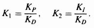
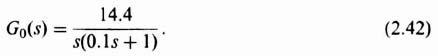
Let us consider the second-order system illustrated in Figure 2.18a. We will assume that the original forward-loop transfer function G₀(s) is given by

The closed-loop transfer function, C(s)/R(s), is given by

or

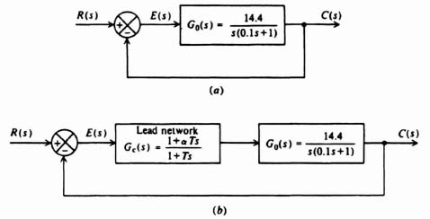
Figure 2.18 Design of a second-order system.

Comparing Eqs. (B.3) and (2.44), we observe that the undamped natural frequency ω_n and damping ratio ζ of the system are given by

and

If the system is subjected to a unit step input, the transient response will have the form shown in Figure B.4 (interpolate between ζ = 0.4 and ζ = 0.6). The maximum percent overshoot can be obtained from Eq. (B.33) and is found to be 23.5%.

Let us assume, for this application, that it is desired to have a critically damped system (ζ = 1). We will demonstrate how this can be achieved using a cascaded network and minor-loop rate feedback.

Figure 2.18b illustrates the form that the system illustrated in Figure 2.18a would have if a cascaded network were used. We attempt to achieve a damping ratio equal to 1 using a phase-lead network, where

As was assumed previously, in Section 2.2, we assume that T αT, and therefore G_c(s) can be approximated by (proportional plus derivative control)

The closed-loop system transfer function for this case was derived in Section 2.2 [see Eq. (2.13)] as

The equivalent damping ratio for this situation was derived in Section 2.2 [see Eq. (2.15)] as

The object in this problem is to design ζ_eq = 1 for the case where

Substituting the values into Eq. (2.49), we find that

We know that the resulting system will be stable and critically damped, and will have a steady-state response error for a unit step input of zero. The steady-state response error of the system to a unit ramp input was derived [see Eqs. (2.18) and (2.20)] as

Let us next attempt to achieve the same type of performance using minor-loop rate feedback. Figure 2.19 illustrates the form that the system illustrated in Figure 2.18a would have if minor-loop feedback were used. Our goal is to achieve a damping ratio of ζ = 1. The closed-loop system transfer function for this case was derived previously, in Section 2.2 [see Eq. (2.26)] as

The equivalent damping ratio for this configuration was derived in Section 2.2 [see Eq. (2.28)] as

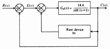
Figure 2.19 Minor-loop feedback added to the system shown in Figure 2.18a.

The object in this problem is to design ζ_eq = 1 for the case where

and

Substituting these values into Eq. (2.53), we find that

Notice that b and αT are identical.

We know that the resulting system will be stable and critically damped, and will have a steady-state response error of zero for a unit step input. The steady-state response error of the system to a unit ramp input was derived [see Eq. (2.31)] as

The increase has been accounted for in Section 2.3; by using a high-pass filter in the feedback path to block a steady-state output from the rate feedback, the steady-state error can be reduced to 0.0695.

2.6. COMPENSATION AND DESIGN USING THE BODE-DIAGRAM METHOD

The techniques necessary to construct and analyze the open-loop frequency response of a feedback control system utilizing the Bode-diagram approach were presented in Section 1.7. This section illustrates how the Bode diagram can be used for designing a feedback-control system in order to meet certain specifications regarding relative stability, transient response, and accuracy. It is important to emphasize that the Bode-diagram approach is used very frequently by the practicing control engineer. Its use is due to the fact that the anticipated theoretical results may be relatively simply checked with actual performance in the laboratory just by opening the feedback loop and obtaining an open-loop frequency response of the system.

Bode's primary contribution to the control art is summarized in two theorems [7]. We introduce the concepts embodied in these theorems first in a qualitative manner, and then the mathematical statements are given.

A. Bode's Theorems

Bode's first theorem essentially states that the slopes of the asymptotic amplitude–log-frequency curve implies a certain corresponding phase shift. For example, in Section 1.7 it was shown that a slope of 20n dB/decade (or 6n dB/octave) corresponded to a phase shift of 90n° for n = 0, ±1, ±2,…. Furthermore, this theorem states that the slope at crossover (where the attenuation-log-frequency curve crosses the 0-dB line) is weighted more heavily toward determining system stability than a slope further removed from this frequency. This results in a rather complex weighting factor which is a measure of relative importance toward determining system stability.

From what has been presented so far, this theorem is intuitively seen to be valid. Gain cross over frequency is one of the two points that is checked to determine the degree of stability when using the Bode diagram. Specifically, the phase shift is measured at this particular frequency in order to determine the phase margin. A feedback system whose slope at gain crossover is −20 dB/decade, and whose other slope sections are relatively far away from crossover in accordance with the relative weighting function, implies a phase shift of approximately −90° in the vicinity of cross over and a corresponding phase margin of about 90°. This value of phase margin certainly implies a stable system. A system, however, whose slope at crossover is −40 dB/decade, and whose other slope sections are relatively far away from crossover in accordance with the relative weighting function, implies a phase shift of approximately −180° and a corresponding phase margin of about 0°. This value of phase margin implies a system which is on the verge of being unstable and would probably be so when actually tested. Steeper slopes would indicate negative phase margins and definitely unstable systems. Therefore, one strives to maintain the slope of the amplitude-log-frequency curve in the area of gain crossover at a slope of −20 dB/decade. Notice that the system, illustrated in Figure 6.33^‡, has slopes of −60 dB/decade that are relatively far from the gain crossover frequency. Therefore, this system has a fairly respectable phase margin of 56.74° by maintaining the 20 dB/decade slope for about an octave below, and about 2 octaves above crossover.

Bode's second theorem essentially states that the amplitude and phase characteristics of linear, minimum-phase-shift systems are uniquely related. When we specify the slope of the amplitude-log-frequency curve over a certain frequency interval, we have also specified the corresponding phase-shift characteristics over that frequency interval. Conversely, if we specify the phase shift over a certain frequency interval, we have also specified the corresponding amplitude-log-frequency characteristic over that frequency interval. The theorem emphasizes the fact that we can specify the amplitude-log-frequency characteristic over a certain interval of frequencies together with the phase-shift-log-frequency characteristics over the remaining frequencies. It should be emphasized that these conclusions apply only if the transfer function is minimum phase.

The second theorem may appear quite trivial at first glance. Its implications however, are quite important. We will make further use of this this theorem when designing feedback control systems using the Bode-diagram approach.

The formal mathematical statement of Bode's first theorem is given by the following expression:

where φ(ω_d) is the phase shift of the system in radians at the desired (e.g., crossover) frequency ω_d, G represents the gain in nepers (1 neper = ln|e|), n = ln(ω/ω_d), |dG/dn| represents the slope of the amplitude-log-frequency curve in nepers per unit change of n (1 neper/unit change of n is equivalent to 20 dB/decade), |dG/dn| is the slope of the amplitude-log-frequency curve at the desired (crossover) frequency ω_d, and ln coth|n/2| is the weighting function which is plotted in Figure 2.20. The first term of Eq. (2.58) represents the phase shift contributed by the slope of the amplitude–log-frequency curve at the reference frequency ω_d. For example, it yields a phase shift of 90° for every neper per unit of n (20 dB/decade). The second term of Eq. (2.58) is proportional to the integral of the product of the weighting function and the difference in slope of the amplitude-log-frequency curve at a frequency ω as compared to its value at the reference frequency, ω_d. Attention is drawn to the fact that it is the weighting function that determines the phase-shift contribution at ω_d due to the amplitude-log-frequency curve which exists at some frequency ω. Because the second term of Eq. (2.58) is zero for large values of n and where n = 0, the value of the integral will be relatively small compared with the first term if the slope of dG/dn is constant over a relatively wide range of frequencies above ω_d. Therefore, under these conditions, the phase shift would be determined primarily by the first term of Eq. (2.58). Following this line of reasoning, the slope of the amplitude-log-frequency curve should be less than −2 nepers per unit of n(−40 dB/decade) over a relatively wide range of frequencies at crossover in order to ensure stability.

The formal mathematical statement of Bode's second theorem is given by the following expression:

Figure 2.20 Plot of the weighting function used in Bode's first theorem.

where ω_s, represents the frequency in radians per second below which the amplitude–log-frequency characteristics is specified and above which the phase characteristic is specified. This theorem emphasizes the interdependence of amplitude and phase shift over the entire range of positive frequencies. In addition, notice that although it is possible to specify amplitude or phase in one range of frequencies, and the other quantity in the remaining frequencies, these quantitites reflect their presence back into the other range of frequencies. Therefore the integration with respect to frequency is performed over the entire range of positive frequencies.

The design of several systems using the Bode-diagram approach is considered next. We shall illustrate a method that determines steady-state accuracy from the Bode diagram as well as meeting relative stability requirements.

B. Example of Phase-Lead and Phase-Lag Network Compensation, and Rate-Feedback Compensation

Let us first consider the third-order system illustrated in Figure 2.21a. Its open-loop transfer function G₀(s) is given by

The Bode diagram for the uncompensated system [G_c(s) = 1] is illustrated in Figure 2.22. It shows a gain crossover frequency of 33.78 rad/sec, a phase margin of −3.402°, and a gain margin of −1.1422 dB. The frequency where the phase shift equals −180° (phase crossover frequency) is 31.7 rad/sec. This Bode diagram was obtained using MATLAB, and is contained in the M-file that is part of my Advanced Modern Control System Theory and Design (AMCSTD) Toolbox which can be retrieved free from The MathWorks, Inc. anonymous FTP server at ftp://ftp.mathworks.com/pub/books/advshinners.

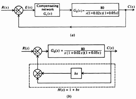
Figure 2.21 A third-order system which is to be compensated using (a) cascade compensation (phase-lag and phase-lead) and (b) rate-feedback compensation.

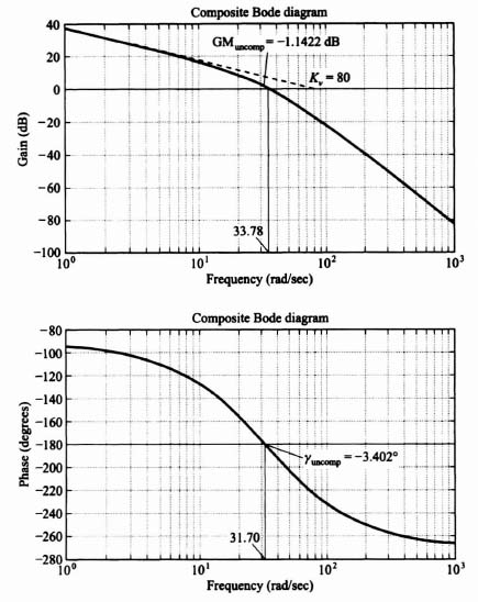
Figure 2.22 Third-order system where the uncompensated transfer function is

These results indicate that the uncompensated system is unstable. Let us next attempt to compensate this system with a phase-lag network, a phase-lead network, and the use of rate feedback in parallel with position feedback (which produces a pure zero factor). The specifications for this sytem require a minimum phase margin of 20° and a minimum gain margin of 10 dB. In addition, it is assumed that a sinusoidal disturbance at 1 rad/sec is present, and a gain of at least 35 dB is required at this frequency to nullify its effect.

1. Phase-Lag Network Compensation Let us first consider the phase-lag-network compensation case in Figure 2.21a. Applying Bode's theorems in order to achieve the specified phase and gain margins, we would expect that the −20 dB decade slope in the vicinity of the new crossover frequency should not extend over too wide a range of frequencies because the relative stability that is desired is rather moderate. The phase-lag network is of the form.

where αT > T. In Section 2.2 we studied the characteristics of the phase-lag network. In particular, Figure 2.9 illustrated the Bode diagram of a general phase-lag network. Notice that this type of network is of such a nature that it attenuated all high-frequency components above ω = 1/T by a factor of 1/α. From the Bode-diagram viewpoint, this attenuating characteristic can be used for stabilization purposes by reshaping the uncompensated amplitude characteristics, so that the initial −20 dB/decade is made to cross over the 0-dB line rather than the −40-dB/decade segment. In other words, one would attempt to stabilize this system with a phase-lag network by placing the frequencies 1/αT and 1/T in the range of frequencies below about 10 rad/sec. It would be desirable that the −20-dB/decade segment start at least around 10 rad/sec cross over the 0-dB line before 20 rad/sec where the amplitude–log-frequency characteristic changes to a slope of −40 dB/decade. In addition, we would not want 1/αT to occur at less than 1 rad/sec, because an open-loop gain of 35 dB has been specified at ω = 1 rad/sec. The final phase of the solution is by means of iteration. However, the procedure converges quite rapidly. Usually, two or three iterations should prove sufficient. For the requirements specified, a phase-lag network given by

results in a gain crossover frequency of 11.371 rad/sec, a phase margin of 20.978° and a gain margin of 10.988 dB as shown in Figure 2.23. The frequency where the phase is −180° (phase crossover frequency) Occurs at 24.22 rad/sec.

2. Phase-Lead Network Compensation. Let us next consider the phase-lead-network compensation case. The lead network has the form

where αT > T. In Section 2.2 we studied the characteristics of the phase-lead network. We assume that any low-frequency attenuation, which is due to the value of 1/α, is made up for by increasing the gain of the feedback control system by a like amount. The Bode diagram of a general phase-lead network was shown in Figure 2.11. From the Bode-diagram viewpoint, this type of characteristic can be used for stabilization purposes by reshaping the uncompensated amplitude characteristics so that a −40-dB/decade slope is made to cross over the 0-dB line along a synthesized −20-dB/decade slope rather than the −40-dB/decade segment. The range of frequencies where one can place the frequencies 1/αT and 1/T is quite limited in this particular problem. The value of 1/αT can be placed between 20 and 33.78 rad/sec, The closer it is to 20 rad/sec, the greater its stabilizing effect. The further away the break 1/T is from 33.78 rad/sec, the greater will be the stabilizing effect of the phase-lead network. It can be seen that this particular solution does not modify the open-loop characteristics in the vicinity of 1 rad/sec and the accuracy specification of 35 dB at 1 rad/sec will easily be achieved.

Figure 2.23 Compensation of a third-order system with a phase-lag network of G_c(s) = (1 + 0.143s)/(1 + s) where the uncompensated transfer function is

We can obtain the pole and zero terms in Eq. (2.63) using a first-cut design procedure by using Eqs. (2.7) and (2.8) for the phase-lead network and the following reasoning. Equation (2.7) states the frequency where the maximum phase lead occurs, and Eq. (2.8) states the maximum value of the phase lead. In view of the analysis of the previous paragraph, it seems reasonable to place the frequency where maximum phase lead occurs around 47 rad/sec, and to make φ_max equal to the phase margin desired (a conservative choice of 28° will be selected) plus the magnitude of the phase margin obtained of the uncompensated system (because it is negative) at the gain crossover frequency of 33.78 rad/sec (3.402°) plus the additional phase shift that the composite phase shift curve incurs in going from the uncompensated crossover frequency of 33.78 rad/sec to ω_max of 47 rad/sec (about 19°) as follows:

Solving these two equations simultaneously, we obtain the phase-lead network

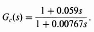
Because this solution has “blinders” on and does not consider the proximity of other poles and zeros, it usually has to be fine-tuned. Therefore, the following phase-lead network was selected and is illustrated in Figure 2.24:

It results in a phase margin of 28.431° and a gain margin of 10.655 dB. This meets the specification requirements. Notice that the resulting phase-lead network has a low-frequency attenuation of 0.005/0.04 which must be made up by increasing the gain by a factor of 0.04/0.005 = 8. Its gain crossover frequency is 47.27 rad/sec, and the phase crossover frequency occurs at 94.06 rad/sec.

If we have a choice of using the phase-lag or phase-lead network, the phase-lag network solution would be preferable because it meets the required specifications with a narrower bandwidth than the phase-lead network case (ω_c = 11.371 rad/sec for the former; ω_c = 47.27 rad/sec for the latter). A feedback control system having a narrower bandwidth will reject a greater amount of noise than one having a wider bandwidth, as well as requiring less power and cost. In addition, the phase-lead network has the disadvantage of requiring a greater amount of amplification within the control system than the phase-lag network. These and other considerations are discussed further in Section 2.10, where tradeoffs of using different kinds of cascade networks and minor-loop feedback compensation methods are compared.

3. Rate Feedback In Parallel with Position Feedback Compensation. Finally, we wish to compensate the system using rate-feedback compensation in parallel with position feedback as shown in Figure 2.21b. The addition of rate feedback provides an H(s) term of

which represents a pure zero term that provides a phase lead of

Figure 2.24 Compensation of a third-order system with a phase-lead network G_c(s) = (1 + 0.04s)/(1 + 0.005s) where the uncompensated transfer function is

Remember that a pure zero term is an ideal compensator. Using a similar procedure as for the design of the phase-lead network, let us assume that we desire an approximate 50° phase lead at a frequency of 50 rad/sec, Therefore,

The use of rate-feedback compensation is illustrated in Figure 2.25 and indicates a phase margin of 31.9728° at the gain crossover frequency of 39.1641 rad/sec. Its gain margin is infinity, because the phase never is −180° except at ω = infinity.

Figure 2.26 illustrates the Bode diagram of the uncompensated system, and the Bode diagram of the compensated systems with a phase-lag network, phase-lead network, and with rate feedback in parallel with position feedback all superimposed on one Bode diagram.

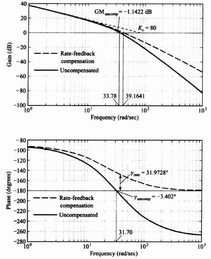
Figure 2.25 Compensation of third-order system with rate feedback (b = 0.0238) in parallel with position feedback where the uncompensated transfer function is

C. Obtaining Steady-State Error Coefficients from the Bode Diagram

The steady-state error coefficients can be determined from the Bode diagram. The definition and importance of these error coefficients have been discussed in Section 5.4^‡. For a system having one pure integration, the velocity constant K_ν can be obtained by extending the initial −20-dB/decade slope until it intersects the 0-dB line. The frequency at which it intersects this line is equal to the velocity constant. In the discussion in Appendix C, K_ν is obtained by letting s approach zero when utilizing the final-value theorem [see Eq. (C.11)]. Therefore, the pole and/or zero terms having the forms (1 + Ts) or [(Ts)² + 2ζTs + 1] all approach unity. This permits one to obtain K_ν directly by considering only the initial slope of the Bode diagram. For the Bode diagram shown in Figures 2.22–2.26, the value K_ν obtained graphically is 80. As a check, using the definition given by Eq. (C.11), we obtain

Figure 2.26 Compensation of a third-order system where the uncompensated transfer function is

Because

then,

It is also interesting to note that the velocity constant is the same for the uncompensated and compensated systems.

For a system which has a double pole at the origin, the acceleration constant K_a can be obtained in a similar manner. The initial −40-dB/decade slope is extended until it intersects the 0-dB line. The square of the frequency at which it intersects this line is equal to the acceleration constant.

D. Example of Compensating a System Containing a Disturbance Input

The next system we consider is illustrated in Figure 2.27. This consists of a third-order system which has an unwanted external input U(s). The open-loop transfer function for the uncompensated system, G₀(s), is given by

It is desired that the steady-state error resulting from an unwanted, external step input signal at U(s), should not exceed 0.1 unit. The compensation device, G_c(s), is to contain amplification which will meet this accuracy requirement together with a phase-lead or phase-lag network which will provide a minimum phase margin of 20° and a minimum gain margin of 6 dB.

The value of gain K required for G_c(s) will be computed first. For this calculation, U(s) is assumed to be the input and E(s) is assumed to be the output. The transfer function between these two points is given by

Setting U(s) = 1/s, we obtain the expression for the Laplace transform of the error, E(s), as

Figure 2.27 A third-order system having an unwanted external input.

The required value of K can be obtained by applying the final-value theorem to E(s) and setting the result equal to 0.1 unit. We find

Let us next determine the compensating network required to achieve a phase margin of 20° and a gain margin of 6 dB. The transfer function of the uncompensated system, with K = 9.55, is given by

Its Bode diagram which is drawn in Figure 2.28, indicates a phase margin of 0.7167° (gain crossover frequency is 5.8668 rad/sec) and a gain margin of 0.267 dB (phase crossover frequency is 5.9522 rad/sec), We wish to increase the phase margin by about 20°. This Bode diagram was obtained using MATLAB and is contained in the M-file that is part of my AMCSTD Toolbox and can be retrieved free from The MathWorks, Inc. anonymous FTP server at ftp://ftp.mathworks.com/pub/books/advshinners.

Figure 2.28 Compensation of a third-order system where

Solid line = uncompensated; dashed line = compensated

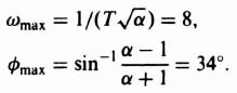
As in the previous problem analyzed in this section, we will estimate the values of ω_max and φ_max for Eqs. (2.7) and (2.8), respectively, to obtain a first-cut design. We must be careful when using this approach, because we actually want to have this phase shift at the gain crossover frequency in order to achieve the desired phase margin. However, specifying α, T, and ω_max does not ensure that φ_max will be at the gain crossover frequency. After obtaining this first-cut design, we then fine-tune the results to obtain the specification requirements as in the previous example. For this design and an analysis of the Bode diagram of the uncompensated system shown in Figure 2.28 a value of ω_max = 8 rad/sec was selected. The value of φ_max selected was a conservative value of 34° which includes the difference between the minimum phase margin desired (20°) and the actual phase margin of the uncompensated system (0.7167°) plus the difference in phase shift between the gain crossover frequency of the uncompensated system (5.8668 rad/sec) and 8 rad/sec plus an extra margin to be conservative. The resulting two equations to be solved simultaneously were

The result is a phase-lead network whose transfer function is

The first-cut design was adjusted a little to better fit the overall Bode diagram and the final phase-lead network selected is as follows:

This network causes a gain crossover frequency of 6.9778 rad/sec where the phase margin is 21.71°, and a gain margin of 7.955 dB (the phase crossover frequency is at 11.5247 rad/sec), This satisfies the specification. Remember that this network will require an increase in the amplifier gain by 3.34 to make up for the attentuation of 0.05/0.167 = 0.2994 that it provides.

E. Example for Compensating a Two-Loop System Using Rate Feedback in Cascade with a Filter

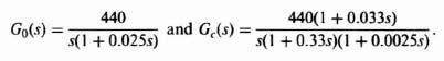
The concluding problem we consider using the Bode-diagram approach consists of designing the feedback control system illustrated in Figure 2.29a. For this particular system, we desire that the steady-state error resulting from a velocity input of 110 rad/sec be equal to 0.25 rad. The uncompensated open-loop transfer function G₀(s) is given by

Figure 2.29 (a) Use of rate feedback in cascade with a high-pass filter in order to compensate a feedback control system. (b) Equivalent block diagram for the system shown in (a).

where K_ν = velocity constant and T_m = motor time constant = 0.025 sec. This transfer function consists of an amplifier, positioning motor, gear train, and load. In order to achieve the required accuracy, K_ν must equal

We want a phase margin of approximately 55° for this system. This will be achieved by means of minor-loop rate-feedback compensation which is cascaded with a simple RC high-pass filter (phase-lead network) in order not to increase the steady-state response error for velocity inputs. This was discussed in Section 2.3 (see Figure 2.15).

The open-loop frequency response we must plot on the Bode diagram is that obtained with the minor-rate loop closed and the outer position loop opened. Therefore, we are interested in obtaining the equivalent transfer function between E(s) and C(s). This is easily found to be

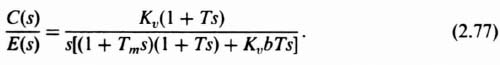
Expanding the denominator of Eq. (2.77), we obtain the expression

This expression can be put into the form

by defining the time constants and T₁ as

and

Therefore, we may redraw Figure 2.29a as shown in Figure 2.29b. For any set of values for T_m, T, K_ν and b, we can derive and T₁ by solving the simultaneous equations (2.80) and (2.81). Another approach is to choose T and T₁ from the Bode diagram which meets the specified phase margin and solve for the required rate-feedback constant b.

The procedure we follow when compensating this system is to draw the Bode diagram for the uncompensated system in accordance with Eq. (2.75) and then fit the characteristics of the compensated system in accordance with

until a phase margin of 55° is achieved. The compensated characteristic will then determine T and T₁, from which and the rate-feedback constant b can be determined. Figure 2.30 illustrates the Bode diagram of the uncompensated and compensated systems. The phase margin of the uncompensated system is 17.1°. Values of

and

result in a phase margin of 55.36°. From Eq. (2.81), the corresponding value of rate-feedback constant b is 0.0186. Figure 2.30 was obtained using MATLAB and is contained in the M-file that is part of my AMCSTD Toolbox.

The type of compensation just illustrated is used quite frequently in practice. In order to really understand what is actually happening, it is important to examine the Bode diagram of Figure 2.30 closely. The net effect of the minor-loop rate feedback has been to move the equivalent motor break frequency from 1/T_m to by the ratio given in Eq. (2.80). This technique is used quite frequently to compensate power servos. The net effect of the phase-lead network, in the minor-loop feedback path, is to appear as a phase lag, for the equivalent open-loop characteristics of Figure 2.29b. This can be easily understood because we effectively see the reciprocal of the feedback element when looking into a closed-loop system which has an open-loop gain much greater than unity [see Eq. (2.122)^‡]. This is a very important fact that can be utilized to approximate the Bode diagram in preliminary designs. This point is now expanded upon in the following section.

Figure 2.30 Compensation of the system shown in Figure 2.29b.

The complete case study for the design of an angular control system for a robot's joint is presented in Section 7.4 of Chapter 7. In this problem, the Bode diagram is used for analyzing and designing the control system.

2.7. APPROXIMATE METHODS FOR PRELIMINARY COMPENSATION AND DESIGN USING THE BODE DIAGRAM

Having presented detailed compensation methods, let us next focus our attention on approximate methods for obtaining a first cut at compensation utilizing the Bode diagram [8–10]. Although the procedures presented in this section are approximate, they are generally adequate for the preliminary stage of design. Before the system design is completed, however, the exact magnitude and phase curves should be drawn as indicated previously. The practice of utilizing approximate methods for preliminary design is generally employed as a convenience in obtaining significant time constants, gains, and phase characteristics required for a design.

A. Approximate Closed-Loop Response from the Bode Diagram

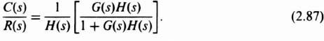
In order to develop the concept of this approach, let us consider the feedback system illustrated in Figure 2.31. The closed-loop transfer function of this system is given by

Let us modify this equation into the following more convenient form:

As shown previously, the magnitude (in decibels) of G(s)H(s) can be approximated by straight lines of constant slope when plotted against frequency on a log scale. Therefore, it appears reasonable that the term 1 + G(s)H(s) in Eq. (2.87) may also be dealt with in a similar approximate manner as follows:

Substituting these approximations into Eq. (2.87), we find that

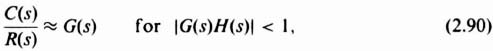
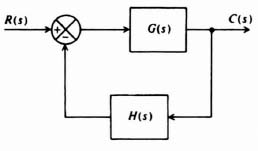
Figure 2.31 A feedback control system.

The approximations of Eqs. (2.90) and (2.91) are very useful as a first cut in the preliminary design of a control system. However, it is important to point out that they are approximate relationships, and are subject to error particularly at those frequencies where G(s)H(s) = 1. However, the amount by which the approximations are in error can be calculated, and this correction can then be applied to correct the approximate value. The resultant corrected value is then an exact solution.

The technique of applying the approximation of Eqs. (2.90) and (2.91) can best be illustrated through an example. Consider the feedback system of Figure 2.31, where and

and

This example will illustrate how feedback, around an element containing a time constant, reduces the time constant of that element. Substituting Eqs. (2.92) and (2.93) into Eq. (2.86), the resultant system transfer function is given by

For purposes of illustration, it is assumed that

in this example. For these values, Figure 2.32 illustrates the straight-line approximations for |C(s)/R(s)|, |G(s)|, and |G(s)H(s)|. The dashed curve representing G(s) [and G(s)H(s) as H(s) = 1] has a gain of 10 (20 dB) for frequencies lower than ω = 1/T = 1 rad/sec. At frequencies higher than ω = 1 rad/sec, G(s) and G(s)H(s) have an attentuation of 20 dB/decade. At , G(s) and G(s)H(s) approximately equal 0 dB. Equation (2.91) indicates that for frequencies lower than ω_n = 10, the system transfer function C(s)/R(s) equals 1/H(s) = 1 and is shown by the solid line at 0 dB. For frequencies greater than ω_n, Eq. (2.90) indicates that C(s)/R(s) is equal to G(s) as shown. Figure 2.32 illustrates very clearly that the use of unity-gain feedback around a single time-constant element results in a reduction in its time constant. This admirable characteristic is achieved at the expense of a loss of gain.

It is important to recognize that the results obtained for the closed-loop transfer function are approximate. For example, Eq. (2.94) indicates that the gain is actually K/(1 + K) = 10/(1 + 10) = 0.909 instead of 1 for ω < ω_n, and the closed-loop time constant is T/(1 + K) = 1/(1 + 10) = 0.0909 instead of . Note that these errors decrease as the gain K increases. Generally, K is quite large and the error between the approximate and exact curves is very small.

The form of Eq. (2.87) is very well suited for determining the value of C(s)/R(s) when |G(s)H(s)| > 1, with the bracketed term representing the difference between the approximate and exact curves. In order to determine a general analytic expression for finding the difference between the approximate and exact curves when |G(s)H(s)| < 1, let us reconsider Eq. (2.86) and rewrite it as follows:

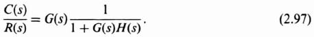
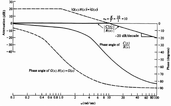
Figure 2.32 Open- and closed-loop gain and phase characterist is for the system of Figure 2.31 where G(s) = 10/(1 + s) and H(s) = 1.

Therefore,

For those frequencies where |G(s)H(s)| < 1, the bracketed term of Eq. (2.98) represents the error between the approximate solution

and the exact solution. Another way of looking at this is that the bracketed term represents a correction factor which can be used to correct the results of the approximation given by Eq. (2.90).

B. The Straight-Line Phase-Shift Approximation

For preliminary design purposes, it is usually sufficient to obtain quantitative information regarding phase shift without resorting to the exact but tedious method of calculating the phase. We have found it convenient to represent the amplitude characteristics by a straight-line approximation, and can utilize a similar technique for the phase-shift function. In order to introduce the method, let us consider the phase shift due to the transfer function representing a zero factor given by

Figure 2.33a illustrates the exact and straight-line approximation and Figure 2.33b illustrates the exact phase shift and its straight-line approximation. The straight-line approximate phase shift has been constructed by drawing a straight line tangent to the actual curve at ω = ω₁.

In order to construct these straight-line phase-shift approximations by inspection, the dependence of ω_A and ω_B on ω₁ must be known. This can be obtained by first considering the slope of the actual curve at ω = ω₁ as follows:

The slope at ω = ω₁ can be obtained by differentiating this expression:

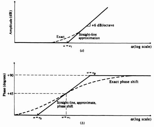
Figure 2.33 Straight-line, approximate, phase-shift methods for a zero factor term.

Knowing the slope at ω = ω₁ the intercepts at ω_A and ω_B can be obtained from

which gives

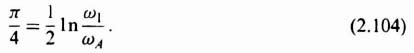
Therefore,

It is interesting to note that if a number other than e were chosen for the logarithmic base, the slope in Eq. (2.105) would change, but the frequency ratio given by Eq. (2.105) would remain the same.

Based on this result, complicated approximate straight-line phase-shift curves can be obtained. Figure 2.34 illustrates the application of this approach for a transfer function given by

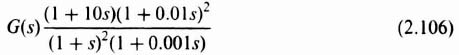
and compares the approximate straight-line phase-shift curve with the exact phase-shift curve. Observe that the errors obtained by using the approximate phase curve are larger than the corresponding errors of the amplitude approximation. However, the use of this approximation greatly aids the control-system engineer in obtaining a first cut preliminary design.

The example just presented contained roots that were all real. What happens if the transfer function contains underdamped quadratic factors? In order to analyze this situation, let us consider the following normalized quadratic phase-lag factor (ζ < 1):

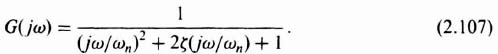
It was shown in Section 6.7^‡ that the amplitude and phase-shift terms are given respectively by [see Eq. (6.92)^‡]:

Figure 2.34 Approximate straight-line phase-shift (solid line) and exact phase-shift (short dash-long dash line) characteristics of

Let us focus attention on the phase-shift term. Differentiation of Eq. (2.109) results in the slope at ω = ω_n being given by

As before, the two intercepts ω_A and ω_B can be found as follows:

Therefore,

Exact phase characteristics corresponding to Eq. (2.107) and its straight-line approximation, based on the relationship of Eq. (2.112), are illustrated in Figure 2.35. In addition, the exact amplitude characteristics of Eq. (2.108) and its straight-line approximation are also illustrated. Observe from Eq. (2.112) that as ζ approaches zero, the two frequency ratios decrease and approach unity in the limits. This certainly agrees with the exact phase characteristics of a quadratic phase lag as illustrated in Figure 6.28^‡. On the other hand, when ζ = 1, the roots become real and Eq. (2.112) reduces to Eq. (2.105).

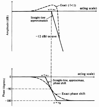
Figure 2.35 Straight-line approximate phase-shift method for a quadratic lag factor (ζ < 1).

The reader is again reminded that the straight-line phase-shift approximation is not exact. It should only be used in order to obtain a first cut for preliminary design work. It should also be noted that the errors of the straight-line phase-shift approximation are generally larger than the corresponding errors of the amplitude approximation. For this reason, the phase-shift approximation is not used for final design. In the final design, the actual phase-shift characteristics must be employed as previously illustrated.

2.8. COMPENSATION AND DESIGN USING THE NICHOLS CHART

The Nichols-chart method has been developed in Section 1.7. We demonstrated in that section how one could obtain the closed-loop frequency response of a feedback control system by superimposing the open-loop gain-phase characteristics onto the Nichols chart. Specifically, we obtained the closed-loop frequency response of the system shown in Figure I1.7-1. The intersections of the open-loop gain-phase characteristics and the Nichols closed-loop gain characteristics were shown in Figure I1.7-2. The resulting closed-loop frequency response was illustrated in Figure I1.7-3. It indicated a maximum value of peaking M_p of 6.758 dB (2.2) and the frequency at which it occurred, ω_p, was 8.989 rad/sec. A value of M_p = 6.758 dB (2.2) does not represent a good design. This section demonstrates how the control engineer may use the Nichols chart in order to achieve a specified performance.

Let us assume for this problem that an acceptable value of M_p is 1.4 (2.92 dB). This may be achieved by adding a phase-lag or phase-lead network in cascade with the forward-loop transfer function G(s). A phase-lag network is used for this problem although a solution can be found as easily using a phase-lead network. We shall demonstrate that for an M_p of 2.92 dB the object is to modify the gain-phase characteristics on the Nichols chart so that it is just tangent to the 2.92 dB locus and does not enter it. By restricting the gain-phase characteristics to areas external to the M = 2.92 dB locus, we will have limited M_p to 2.92 dB, because the interior of this locus represents values of M greater than 2.92 dB.

Studying the characteristics of Figure I1.7-2, we see that relatively large magnitudes of G(jω) exist for ω < 3 rad/sec. Therefore, it is not desirable to shift these magnitudes inside the M_p = 2.92 dB curve. In addition, it is desirable to attenuate G(jω) by a factor of about 3 in the range of frequencies of ω = 5 − 12 rad/sec. A phase-lag network, (1 + Ts)/(1 + αTs), whose factor α equals 3 will achieve this if is chosen at about 1 rad/sec, Solving for αT and T, we get αT = 1.74 and T = 0.58.

In order to obtain the gain-phase characteristics of the open-loop system, the Bode diagram is first drawn as indicated in Figure 2.36. Then for each value of ω the magnitude and phase of the open-loop compensated characteristics are plotted into a Nichols chart as shown in Figure 2.37. Because the open-loop gain-phase characteristics are just tangent to the constant-magnitude locus corresponding to M = 2.976 dB (1.4), we have achieved our goal. Notice that we have shifted ω = 1 rad/sec by about −35°, but this does not increase M_p. Figures 2.36 and 2.37 were obtained using MATLAB, and are contained in the M-files that are part of my AMCSTD Toolbox. It is important to note that the use of MATLAB and the AMCSTD Toolbox permits one to obtain the Nichols chart directly without having to first obtain the Bode diagram.

2.9. COMPENSATION AND DESIGN USING THE ROOT-LOCUS METHOD

The root-locus technique has been developed previously in Sections 1.7, and MATLAB computer programs for obtaining the root locus were also presented in Section 1.7. It is a very helpful tool that the control engineer can use in order to study the variation of gain, system parameters, and effect of compensation. We demonstrated in Section 1.7 the migration of poles in the complex plane as the gain of the system was varied from zero to infinity. We obtained the root locus for several feedback systems including the following in Ilustrative Problem I1.10:

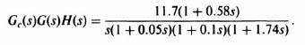
Figure 2.36 Bode diagram for the compensated system of Figure I1.7-1, where

This was illustrated in Figure I1.10. An analysis of the root locus for this system indicated that it was always unstable, because at least one of the roots of the characteristic equation always occurred in the right-half-plane. This section demonstrates how this system may be compensated by means of a phase-lead network, and/or rate feedback in parallel with position feedback. This problem is followed by considering phase-lag-network compensation for the system illustrated in Figure I1.9. In addition, we shall demonstrate how the control engineer may determine the transient response of the compensated systems in order to meet certain specifications.

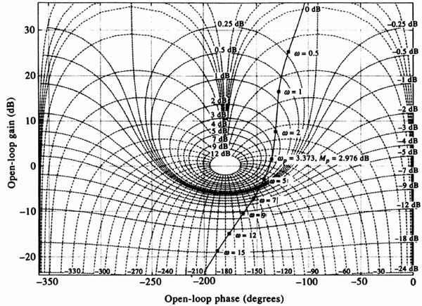
Figure 2.37 Compensation of the system shown in Figure I1.7-1 for M = 2.976 dB(1.4).

A. Example of Phase-Lead Network and Rate-Feedback Compensation

Let us attempt to stabilize the system of Figure I1.10 by means of a phase-lead network in cascade with the forward-loop transfer function. The form of its transfer function is given by

We assume that the effect of the pole introduced by the phase-lead network has a negligible effect compared with its zero. Therefore, we assume that the transfer function of the cascaded phase-lead network can be approximated by the zero term only, which is also equivalent to the pure zero obtained with rate feedback in parallel with position feedback (see Figure 2.14a):

The resulting value of G_c(s)G(s)H(s), which is to be examined on the root locus, is given by

We wish to investigate the effect on stability of a variation in α as follows:

The resulting root loci for all these cases are presented next. It is important to emphasize at this point that, although we make use of most of the anlaytic tools developed in Section 1.7, we do not use all of them, This omission is due to the fact that some of the analytic techniques developed are too complex to use for higher-order systems. For example, it is very tedious to determine the value of the gain K along the root loci utilizing the relationship given by Eq. (6.133)^‡. Fortunately, this can be obtained much more easily by using MATLAB (Section 1.7). The approach taken in presenting the resulting root loci for this problem is to outline the results of the 12 rules developed previously in Section 6.14^‡, and use MATLAB (Section 1.7) wherever it is helpful. In addition, the values of gain obtained using MATLAB which are pertinent for an intelligent evaluation of the problem will be indicated. It is my feeling that this dual approach is the best procedure to use when explaining the root-locus method. This de tailed analysis will be applied to all five cases.

Case A. α = 0.5. See Figure 2.38 for the root-locus sketch.

Rule 1. There are four separate loci because the characteristic equation,

is a fourth-order equation.

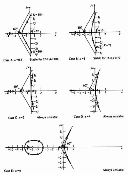
Figure 2.38 Compensation of the root locus shown in Figure I1.10 using a pure zero term where G_c(s) = (s + α).

Rule 2. The root locus starts (K = 0) from the poles located at 1, −1, and a double pole at −4. One branch terminates (K = ∞) at the zero located at α = −0.5 and three branches terminate at zeros located at infinity.

Rule 3. Complex portions of the root locus occur in complex-conjugate pairs.

Rule 4. The portions of the real axis between 1 to −α, −1 to −4, and −4 to ∞ are part of the root locus.

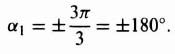
Rule 5. The branches approach infinity as K becomes large at angles given by

and

Rule 6. The intersection of the asymptotic lines and the real axis occur at

Rule 7. Using MATLAB, we found the point of breakaway from the real axis to occur at −1.7549.

Rule 8. Using MATLAB, we found the intersection of the root locus and the imaginary axis to occur at s = ±j3.3, where the gain is 104, and at the origin, where the gain is 32.

Rule 9. This rule does not apply here.

Rule 10. This rule shows that as certain of the loci turn to the right, others turn to the left to ensure that the sum of the roots is a constant.

Rule 11. This rule does not apply here.

Rule 12. The root locus does not cross itself.

The resulting root locus indicates that the system is stable when 32 < K < 104.

Case B. α = 1. See Figure 2.38 for the root-locus sketch. A zero at s = −1 cancels the pole at −1. The resulting root-locus sketch indicates that this system is stable when 16 < K < 72. (The point of breakaway occurs at −0.667.)

Case C. α = 2. See Figure 2.38 for the root-locus sketch. The resulting root-locus sketch indicates that the system is always unstable, because at least one of the roots of the characteristic equation always occurs in the right half-plane except for the condition where two poles exist at the origin. (The point of breakaway occurs at the origin.)

Case D. α = 4. See Figure 2.38 for the root-locus sketch. A zero at α = 4 cancels one of the poles located at −4, the resulting root-locus sketch indicates that the system is always unstable since at least one of the roots of the characteristic equation always occurs in the right half-plane. (The point of breakaway occurs at 0.1196.)

Case E. α = 6. See Figure 2.38 for the root-locus sketch. The resulting root-locus sketch indicates that the system is always unstable, because at least one of the roots of the characteristic equation always occurs in the right half-plane. (The points of breakway occur at 0.1156 and −4, and a break-in occurs at −7.0611.)

Conclusions of Cases A through E

Interpretation of Figure 2.38 is quite interesting and revealing. It indicates that the exact location of the zero is very important from a stability viewpoint. Cases A and B were the only configurations which had regions of stability. As a matter of fact, the closer the zero lies to the imaginary axis, the greater is its stabilizing effect. This point is very important. Because Case A resulted in larger values of gain, it would result in a more accurate system and is, therefore, preferred to Case B.

The reader should not get the impression that α could be made extremely small (e.g. 0.0001) to satisfy this guideline because you will be paying a penalty in the size of the capacitors and resistors used in a passive phase-lead network. Remember that the form of the zero is (s + α), which can be modified to α[(1/α)s + 1], where 1/α is the time constant of the zero term. Therefore, very small values of α mean that the values of the components (resistors and capacitors) would be too large which is undesirable from a practical viewpoint. If the zero term (s + α) is obtained using rate feedback in cascade with position feedback, as in Figure 2.14a, then you would have to make 1/α = b and very small values of α would mean extremely large values of b. This would require an amplifier in cascade with the rate-feedback sensor (e.g., tachometer or rate gyro), which is undesirable due to the added cost and possible noise problems.

B. Determination of the Transient Response

The transient response of the system can also be obtained by reasoning along these lines: The transient performance is often dominated by the pair of complex conjugate poles located closest to the origin. This occurs when the other poles are far to the left of the dominant poles, or the other poles are near a zero. The resulting transient components due to these other poles are small under these conditions and diminish rapidly. For this case, the poles closest to the origin are conventionally referred to as the dominant poles. The relative dominance of the closed-loop poles is found from the ratio of the real parts of the complex-conjugate poles. As a general guideline, reasonable dominance exists if the ratios of the real parts are at least five, and there are no zeros nearby. For such conditions, the closed-loop complex-conjugate poles closest to the origin will dominate the transient response. From the discussion of Appendix B, the expression associated with these complex poles can be given by the following expression [see Eq. (B.3)]:

where ζ = damping ratio, and ω_n = undamped natural frequency. We found in Appendix B that the transient response to a unit step input, for ζ < 1, is given by the following expression [see Eq. (B.24)]:

where

Figure (B.3) illustrated the complex-plane location of these dominant poles. The values derived for the time to the first peak [see Eq. (B.29)] and maximum percent overshoot [see Eq. (B.33)] are specifically for a second-order system whose closed-loop transfer function is given by Eq. (2.117). These quantities change if other closed-loop poles and zeros exist in addition to the dominant complex pair. However, if the ratios of the real parts of the various complex-conjugate poles are greater than five and there are no zeros nearby, then the approximation gives reasonable results. The damping ratio determined in this case using the pair of complex-conjugate roots closest to the imaginary axis is defined as the relative damping ratio of the control system.

Expressions for time to the first peak and percent overshoot, which consider other poles and zeros and give more accurate results, can be derived [6]. These expressions assume that

1. Other poles are far to the left of the dominant poles, so that the amplitude of transients due to these other poles is small.
2. Poles which are not far to the left of the dominant poles are near a zero so that the transient amplitude due to such poles is small.

The expressions, for unity-feedback systems, are given by

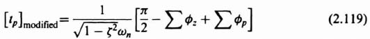
where

= sum of the angles from the zeros of C/R to one of the dominant poles,

= sum of the angles from the poles of C/R to one of the dominant poles,

and the maximum percent overshoot

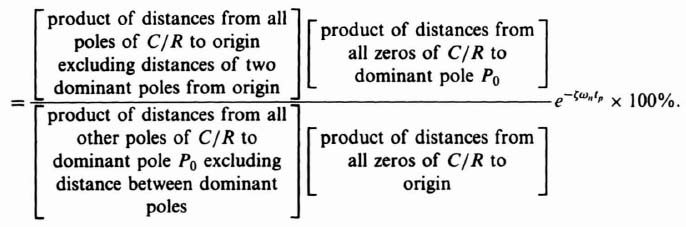
The expression for maximum percent overshoot can be stated symbolically as

where the first set of brackets represents the product of the ratios of the values of s at which poles occur to their absolute distances from the dominant pole. The second set of brackets represents the product of the ratios of the absolute distances of the zeros from the dominant pole and the values of s at which the zeros occur. Let us next apply these expressions in the following design problem.

C. Example of Phase-Lag-Network Compensation and Overall System Performance

The concluding design problem we consider using the root locus consists of employing cascaded phase-lag compensation in order to improve the steady-state performance of a feedback control system. The object is to increase its gain while maintaining a good dynamic response. Specifically, we consider the system whose root locus was illustrated in Figure I1.9. For this system

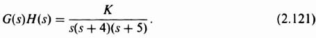
The root locus of Figure I1.9 indicated that the system was stable when 0 < K < 180. Let us assume that a darning ratio of 0.707 achieves a desirable dynamic response for this system. In addition, we must maintain a velocity constant K_ν of 30 in order to meet specified accuracy requirments. Analyzing this problem, by means of the root locus, we can find the value of K which will give the required damping ratio. For example, the redrawn version of Figure I1.9 shown in Figure 2.39 indicates that a K = 21.59 will result in a damping ratio of 0.707 (α = cos⁻¹ 0.707 = 45°). This value of gain does not maintain the required velocity constant of 30. The actual value of K_ν resulting from K = 21.59 is

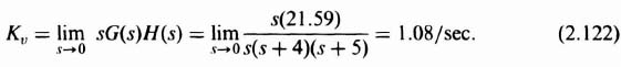
It is therefore clear that we cannot just increase the gain K to a value that produces the required velocity constant, because this would decrease the damping ratio and adversely affect the transient response or cause the system to become unstable. Using the root locus for a solution, we show how these two conflicting factors can be resolved.

In order to achieve the specification requirements, we must increase the gain, but at the same time maintain the dominant complex-conjugate roots of the root locus where the value of K = 21.59 is shown in Figure 2.39 so that the damping ratio of 0.707 is maintained. We can accomplish this with a phase-lag network and an increase in the system gain.

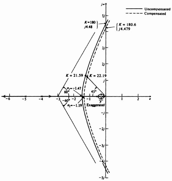
Figure 2.39 Compensation of the root locus shown in Figure I1.9 using a cascaded phase-lag network and an increase in gain.

Let us assume that the combined transfer function representing the increase in gain (n) and the phase-lag network is given by

The form of Eq. (2.123) indicates that this compensator provides a low-frequency gain of n in addition to the phase lag, where n is also the ratio of the break frequencies. The open-loop transfer function of the compensated system is given by

In general, the distances of nα and α from the origin in the s-plane are chosen to be small compared with the distances of the other zeros and poles of the uncompensated open-loop transfer function, so that the added pole and zero of the compensator will not contribute significant phase lag in the vicinity of the gain crossover frequency. This result is quite clear from a study of the Bode diagram, which we shall shortly do at the conclusion of this design (see Figure 2.40). Certainly we do not wish to add the phase-lag contribution in the vicinity of the gain crossover frequency. Therefore, the combination of pole and zero will be quite close together on the root locus and very close to the origin. The combination is usually called a dipole.

In order to complete the design, α is chosen close to the origin at 0.01 and n is chosen, using the following derivation, to achieve a K_ν = 30:

Substituting Eq. (2.124) into Eq. (2.125), we obtain

or

Because we desire that K = 21.59 from a transient viewpoint, we must have

The completed root locus for the compensated system whose open-loop transfer function is given by

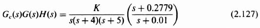
must now be determined. Because the dipole is added near the origin, the original root locus is not changed significantly, because the two poles and the zero near the origin tend to merge into a single pole.

Let us next determine the new resulting root locus, which is shown as the dashed curve in Figure 2.39, and analyze the effect of the dipole on it. Specifically, we wish to know whether the new root locus will indeed have K_ν = 30. In addition, we would like to determine the transient response of the compensated system. Each of the 12 rules for constructing the root locus will be considered.

Rule 1. There are four separate branches, because the characteristic equation.

is a fourth-order equation.

Rule 2. The root locus starts (K = 0) from the poles located at the origin, −0.01, −4, and −5. One branch terminates (K = ∞) at the zero located at −0.2779 and the other three branches terminate at zeros which are located at infinity.

Rule 3. Complex portions of the root locus occur in complex-conjugate pairs.

Rule 4. The portions of the real axis between the origin and −0.01, −0.2779 and −4, and −5 to −∞ are parts of the root locus.

Rule 5. The four branches approach infinity as K becomes large at angles given by

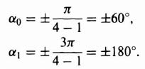
Rule 6. The intersection of the aymptotic lines and the real axis occurs at

Rule 7. The point of breakaway from the real axis can be computed from the following equation:

where

β₁ = angle from the zero at −0.2779 to the point s₁, that is located a small distance δ off the positive real axis,

β₂ = angle from the pole at the origin to the point s₁.

β₃ = angle from the pole at −0.01 to the point s₁.

β₄ = angle from the pole at −4 to the point s₁,

β₅ = angle from the pole at −5 to the point s₁.

The equation of the transition of the root locus from the real axis to a point s₁ which is a small distance δ off the axis is given by

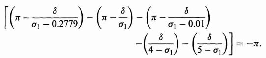
Solving, we obtain σ₁ = −1.19, which compares with a value of −1.47 obtained using MATLAB for the uncompensated system.

Rule 8. The intersection of the root locus and the imaginary axis can be determined by applying the Routh–Hurwitz stability criterion to the characteristic equation

which becomes

The resulting Routh–Hurwitz array is given by

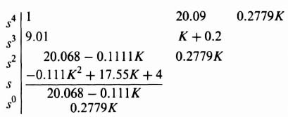
An interesting situation occurs in this Routh–Hurwitz array, because the first terms of the third and fourth rows can go to zero for certain values of gain, K. When the equation

is satisfied, then a possible solution is

When the equation

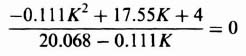
is satisfied, then a possible solution is

Therefore, in order to find which is (or are) valid, let us substitute s = jω into the characteristic equation and find out where the root locus crosses the imaginary axis. The results can be separated into a real and imaginary part and written in the following form:

For K to be real and imaginary parts of this equation must each equal zero. Therefore, from the imaginary part:

Now, to find the value of K which corresponds to this value of crossing of the imaginary axis, let us substitute this value of ω into the real part of Eq. (2.128). The result is the following equation:

Therefore, we find that

is the only possible real value of gain when the root locus crosses the imaginary axis. The analysis indicates that the maximum value of gain, before the system becomes unstable, is 180.6. In Figure I1.9, we found that the uncompensated system had a maximum allowable gain of 180. Therefore, this result indicates that the dipole has an effect on the maximum allowed gain. The corresponding value of s occuring at the crossing of the imaginary axis is found to be ±j4.479 by substituting K_max into the equation for ω. This compares with a value of s = j4.48 obtained previously for the uncompensated case [see Figure I1.9].

Rule 9. This rule does not apply to this problem.

Rule 10. This rule shows that as certain of the loci turn to the right, others turn to the left to ensure that the sum of the roots is a constant.

Rule 11. This rule is quite important to us in this case, because we want to determine the value of gain when ζ = 0.707 (the intersection of a line making an angle of +45° with the negative real axis and the dashed curve). For the uncompensated case, we found that K = 21.59. The new value can be obtained from the following expression:

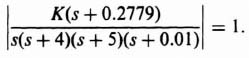
Measuring the distance from the various poles and zeros to the point of interest, we obtain

Therefore, the gain has increased slightly from 21.59 to 22.19. This will result in a slight increase of K_ν from 30 to 30.8.

Rule 12. The root locus does not cross itself.

To conclude this problem, we can calculate the value of the time to the first peak and the maximum percent overshoot from Eqs. (2.119) and (2.120), respectively. These results can then be compared with the values obtained from Eqs. (B.29) and (B.33), which assumes that the transient response is completely controlled only by the pair of complex-conjugate poles located closest to the origin. The time to the first peak of the compensated system can be calculated from Eq. (2.119). In order to use this equation, the location of the other two roots must be determined. Using MATLAB for determining the root locus, these were found to be located at −6.45 and −0.26. Therefore,

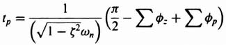
where

ζ = 0.707,

ω_n = 1.63 (distance from the origin of the complex plane to the two dominant poles located at −1.15 ± j1.15—dashed curve of Figure 2.39),

= 141° = 2.47 rad,

= 136° + 90° + 14° = 240° = 4.19 rad.

Substituting these values into the equation for t_p, we obtain

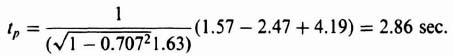
Therefore, the time to the first peak is 2.86 sec. If one simply assumes that the transient response is governed by the pair of complex-conjugate poles located at 1.15 ± j1.15 and uses Eq. (4.29)^‡ to determine the time to the first peak, then the following is obtained:

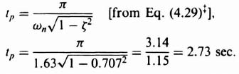
Therefore, we see the slightly improved accuracy obtained using Eq. (2.119).

A similar analysis of the uncompensated system, utilizing Eq. (2.119), results in a time to the first peak of 2.81 sec. For this case, the two complex-conjugate poles are located at −1.2 ± j1.2. The third root can be determined analytically from rule 10:

Therefore,

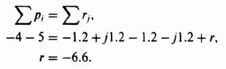
where

ζ = 0.707,

ω_n = 1.7 (distance from the origin of the complex plane to the two dominant poles—solid curve of Figure 2.39),

= 0,

= 90° + 13° = 103° = 1.8 rad.

Hence,

Observe that the dipole compensation increases the time to the first peak slightly.

The maximum percent overshoot of the compensated system can be obtained from Eq. (2.120). To use this equation, we have to determine the location of the other two roots. As mentioned previously, these were found to be at −6.45 and −0.26. Therefore,

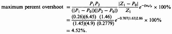
Therefore, the resulting maximum percent overshoot is only 4.52%. If one simply assumes that the transient response is governed by the pair of complex-conjugate poles located at −1.15 ± j1.15 and uses Eq. (B.33) to determine the maximum percent overshoot, then the following is obtained:

Therefore, we see the slightly increased accuracy obtained using Eq. (2.120).

A similar analysis of the uncompensated system utilizing Eq. (2.120) results in a maximum percent overshoot of 4.48%; for this case, the third root is located at −6.6 as illustrated before:

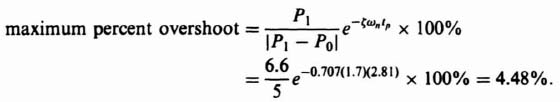
Observe that the dipole compensation increases the maximum percent overshoot slightly.

The results of the transient analysis indicate that the effect of the dipole is to increase the time to the first peak slightly and to increase the maximum overshoot slightly. Of most importance, the dipole increases the velocity constant greatly, from 1.08 to 30.8.

One should note that the dominant pole concept is very useful here, the results coming quite close to the more accurate calculation. In fact, due to the ever-present uncertainty of the parameters of the actual system, it is rarely, if ever, necessary to carry out the detailed calculations indicated.

D. Comparison of the Root-Locus Method with Bode Diagrams

In our analysis of the system whose transfer function was given by Eq. (2.121) and illustrated in Figure 2.39 using the root-locus method, it was pointed out that this same system's analysis using the Bode diagram would be very interesting. It is always interesting to compare the analysis of a system using more than one of the techniques shown as was discussed in Section 6.20^‡, where 12 commonly used transfer functions were compared from the viewpoints of the Nyquist-diagram, Bode-diagram, Nichols-chart, and root-locus methods. In this problem, it is especially useful because the root-locus solution may be difficult to comprehend initially. What did we really do when we kept the dominant complex-conjugate roots almost fixed, increased the gain and added a phase-lag network? It is very clear if we look at the uncompensated and compensated systems from the viewpoint of the Bode diagram. For purposes of the Bode-diagram analysis, the value of K in Eq. (2.121) is set equal to 21.59, and this equation is modified to the following easier form for a Bode diagram:

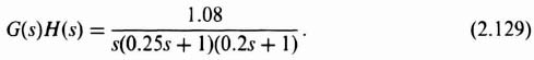
The Bode diagram of the uncompensated system is shown in Figure 2.40. This Bode diagram was obtained using MATLAB (see Section 1.7) and is contained in the M-file part of my AMCSTD Toolbox disk and can be retrieved free from The MathWorks, Inc. anonymous FTP server at ftp://ftp.mathworks.com/pub/books/advshinners. Notice from this diagram that the system has a gain crossover frequency of 1.025 rad/sec, a phase margin of 64.04°, and a gain margin of 18.42 dB (phase crossover frequency occurs at 4.472 rad/sec), Extension of the initial −20-dB/decade slope intersects the 0-dB line at 1.08 rad/sec indicating a K_ν of 1.08 which agrees with Eq. (2.122). (The actual curve intersects the 0-dB line at 1.025 rad/sec.) We now wish to plot the Bode diagram of the compensated system whose transfer function is given by Eq. (2.127). We let K = 22.19 and modify Eq. (2.127) into the following equation which is easier to use for the Bode diagram:

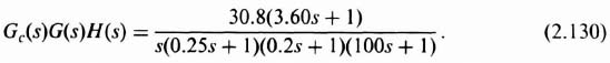
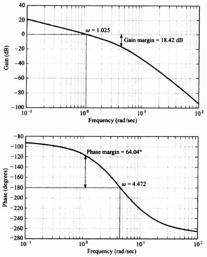
Figure 2.40 Bode diagram for the uncompensated system whose root locus is shown in Figure 2.39.

The resulting Bode diagram for the compensated system, also obtained using MATLAB, whose transfer function is given by Eq. (2.130) is shown in Figure 2.41. It has a gain crossover frequency of 1.138 rad/sec which is close to that of the uncompensated system whose Bode diagram is shown in Figure 2.40 (1.025 rad/sec), because we hardly moved the dominant complex-conjugate poles (see Figure 2.39) in going from the uncompensated to the compensated system. The phase margin of the compensated system is 49.21° (compared to 64.04° of the uncompensated system), and the gain margin of the compensated system is 16.67 dB (compared to 18.42 dB of the uncompensated system). Therefore, the uncompensated system and the compensated system have almost the same relative stability, and about the same gain crossover frequency. From the root-locus viewpoint, this means that the damping factor has hardly changed in going from the uncompensated to compensated systems. (Figure 2.39 shows that the damping factor remains constant at 0.707). However, the velocity constant of the compensated system is 30.8 [see Figure 2.41] compared to the velocity constant of the uncompensated system which is 1.08 [see Eq. (2.122)]. In conclusion, the comparison of the stabilization of this problem using the root locus (Figure 2.39) and the Bode diagram (Figures 2.40 and 2.41) is very interesting as the information shown in the root-locus and Bode diagrams complement each other.

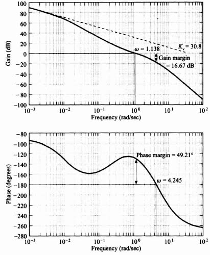
Figure 2.41 Bode diagram for the compensated system whose root locus is shown in Figure 2.39.

2.10. TRADEOFFS OF USING VARIOUS CASCADE-COMPENSATION METHODS AND MINOR-LOOP FEEDBACK

This chapter has presented the use of phase-lag, phase-lead, and phase-lag–lead cascade compensation networks, and minor-loop feedback, compensation (such as rate feedback). The question arises as to which compensation method should be used: cascade compensation or minor-loop feedback compensation. If the answer turns out to be cascade compensation, the question arises as to whether we should use phase-lag, phase-lead, or phase-lag–lead networks? This section addresses these reasonable questions by discussing the tradeoffs of these different methods of compensation, and guidelines are provided for the practical design of control systems.

I cannot provide a simple answer as to what compensation approach is the “best” method to use. Table 2.2 [11] compares the advantages and disadvantages of phase-lag, phase-lead, and phase-lag–lead networks, and minor-loop rate feedback for compensation. They are compared on the basis of characteristics, performance, applicability, and relative cost. Each of these four approaches will improve system stability if used properly, as shown in Chapters 1 and 2. Therefore, each system must be considered separately in order to determine the most effective, optimum, or “best” approach.

Table 2.2. Comparison of Compensation Methods [11]

Reprinted from Control Engineering, May 1978. © Copyright Cahners Publishing Company.

If the system specification requires the need for a low-noise (”quiet”) control system having a small steady-state error, then the phase-lag-network approach is the most desirable from the viewpoints of performance and cost. The phase-lead network is desirable for systems requiring a very fast response, and if the resulting increase in high-frequency noise is tolerable. The phase-lag–lead network has essentially the advantages in performance of both the phase-lag and phase-lead networks. It can result in control systems which are very fast, on a relative basis, and they can result in very small steady-state errors.

Minor-loop feedback compensation using rate-feedback from tachometers and rate gyros has the advantage that it results in a pure zero, when connected in parallel with the position feedback, and represents ideal compensation. Rate-compensating devices have the additional advantage of only requiring a small volume and they are relatively independent of the environmental conditions in which they are operating such as temperature, humidity, and altitude. This is advantageous for control systems operating in space vehicles, airplanes, and ships. For example, if a phase-lead network were used in a hostile environment, the possible use of very large resistors and capacitors could result in very large time-constant variations causing a stable control system to behave as a conditionally stable control system.

In trading off the advantages and disadvantages of minor-loop feedback compensation, it should be emphasized that although they result in systems having the highest performance, this approach is usually also the most expensive. However, in some cases, it may be the only and “best” way to go.

In the practical world of control-system applications, each case is not so straight-forward that the control-system engineer can merely go to Table 2.2 and choose an approach clearly. Conflicting system requirements will usually direct the control-system engineer to more than one possible solution, and neither one of them may be the “best” method. In the final design, the choice of the compensating approach will usually be a compromise based on the tradeoffs considered.

The control-system engineer will usually select the approach based on his or her experience, subjective personal preferences, and the availability of components. As was discussed in the case of choosing the “best” method for stability analysis in Section 6.22^‡, all of the compensation methods should be considered before one is selected. Then the “best” or most effective technique can be selected by the control-system engineer for the final design.

2.11. ILLUSTRATIVE PROBLEMS AND SOLUTIONS

This section provides a set of illustrative problems and their solutions to supplement the material presented in Chapter 2.

1. I2.1. A closed-loop unity-feedback control system used to position a load has a forward transfer function given by

   

   The time constant of the open-loop process is 2 sec. Determine the time constant of the closed-loop control system.

   SOLUTION:

   

   Therefore,

   

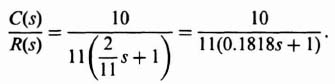
   So, the time constant of the closed-loop control system is 0.1818 sec.

2. I2.2. We wish to analyze the performance of a unity-feedback second-order control system whose forward transfer function represents a process, G_p(s), given by:

   

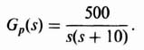
   1. Determine the gain crossover frequency, ω_c, analytically without using the graphical Bode plot.
   2. Determine the phase margin and gain margin of this control system analytically without using the graphical Bode plot.
   3. A phase-lead network compensation, G_c(s), given by

      

      is to be added in series with the process' transfer function, G_p(s). Determine the values of a and T in order that the zero factor of G_c(s) cancels the pole of G_p(s) at s = −10, and the damping ratio of the control system is unity.

   4. Determine the gain crossover frequency, ω_c, analytically without using the graphical Bode plot for the compensated control system.
   5. Determine the phase margin and gain margin of this control system analytically without using the graphical Bode plot.

   SOLUTION:

   1. 

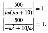
      Solving, we find that the gain crossover frequency, ω_c, equals 21.27 radians per second.

   2. 

      Therefore, the phase margin, γ, equals 180° + φ(ω) = 24.3°.

      The gain margin equals infinity because the phase of φ(ω) is always less than −180°.

   3. 

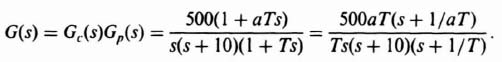
      Therefore, we make

      

      The characteristic equation of the resulting control system is determined as follows:

      

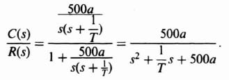
      Therefore, comparing the denominator of this equation with Eq. (B.3):

      

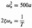
      where ζ = 1. Solving these two equations simultaneously and the previous result that 1/aT = 10, we find that a = 20 and T = 0.005. Therefore,

      

   4. 

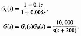
      Solving, we find that the gain crossover frequency of the compensated control system, ω_c, equals 48.6 rad/sec.

   5. 

      Therefore, the phase margin, γ, equals 180° + φ(ω) = 76.34°. The gain margin equals infinity because the phase of φ/(ω) is always less than 180°.

3. I2.3. Due to the inherent instability of a control system containing only a double integration, we wish to add a phase-lead network to the following control system:

   

   Figure I2.3i

   Due to accuracy considerations, we desire the gain of the control system, K, to be 229.6. Due to component considerations, we wish the pole of the phase-lead network, b, to be located at 27. Using the root-locus method, determine the value of the zero of the phase-lead network, a, if the dominant poles of this control system are located at −5.288 + 5.288j and −5.288 − 5.288j.

   SOLUTION: The root locus for this problem is given by the plot in Figure I2.3ii.

   We know that the absolute value of the open-loop transfer function, G₁(s)G₂(s) must equal one. Therefore,

   

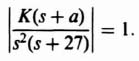
   This equation can be written as follows for K = 229.6 and at s = −5.288 + 5.288j:

   

   Figure 1.23ii

   

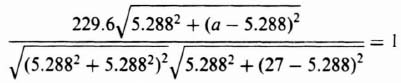
   Therefore, a = −4.

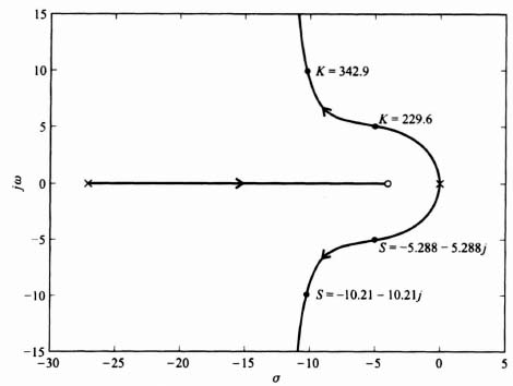
PROBLEMS

1. 2.1. Determine the circuit structure, the values of resistance and capitance, the gains of any amplifiers required, and the complex-plane plot for first-order networks having the following characteristics:
   1. Phase lead of 60° at ω = 4 rad/sec, a minimum input impedance of 50,000 Ω, and an attentuation of 10 dB at dc.
   2. Phase lag of 60° at ω = 4 rad/sec, a minimum input impedance of 50,000 Ω, and a high-frequency attenuation of 10 dB.
   3. A phase-lag–lead network having an attenuation of 10 dB for a frequency range of ω = 1 to ω = 10 rad/sec and an input impedance of 50,000 Ω.

      In all cases, limit the maximum values of resistance to 1 MΩ and capitance to 10 μF. Furthermore, assume that the loads on the networks have essentially infinite impedance.

2. 2.2. The system illustrated in Figure P2.2 consists of a unity-feedback loop containing a minor-rate-feedback loop.

   

   Figure P2.2

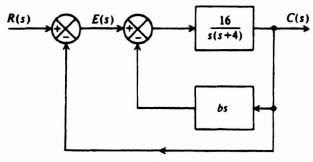
   1. Without any rate feedback (b = 0), determine the damping ratio, undamped natural frequency, peak overshoot of the system to a unit step input, and the steady-state error resulting from a unit ramp input.
   2. Determine the rate-feedback constant b which will increase the equivalent damping ratio of the system to 0.8.
   3. With rate feedback and a damping ratio of 0.8, determine the maximum percent overshoot of the system to a unit step input and the steady-state error resulting from a unit ramp input.
   4. Illustrate how the resulting steady-state error of the system with rate feedback to ramp inputs can be reduced to the same level if rate feedback were not used, and still maintain a damping factor of 0.8.
3. 2.3. Repeat Problem 2.2 for the forward transfer function of the system given by 20/s(1 + s).
4. 2.4. Figure P2.4 illustrates the block diagram of a roll control system used to limit the roll rate excursions of a missile by providing sufficient dynamic reaction to disturbing moments [12]. The disturbance moments result from changes in bank angle and steering control deflections. The basic limitation which determines the effectiveness of the roll-control system is the response of the aileron servo.

   

   Figure P2.4

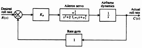
   1. Determine the transfer function, C(s)/R(s), of the system illustrated in Figure P2.4.
   2. Because the transient response is governed by a pair of dominant complex-conjugate poles, specify the requirements of the aileron servo parameters in order that the equivalent damping ratio of the system is approximately 0.5, and the equivalent undamped natural frequency of the system is approximately 4 rad/sec.
5. 2.5. A unity-feedback system has a forward transfer function given by

   

   It is desired to compensate this system so that the resulting damping ratio is unity (critically damped).

   1. Using the classical approach, determine the time constant of a cascaded phase-lead network, containing a zero factor only, that can achieve this.
   2. Using the classical approach, determine the rate-feedback constant of a minor rate-feedback loop which can achieve critical damping.
6. 2.6. Repeat Problem 2.5 for the forward transfer function of the system given by

   

7. 2.7. A phase-lag–lead network, whose general transfer function is given by Eq. (2.9), and whose gain and phase characteristics are illustrated in Figure 2.13, provides a phase lag at low frequencies and a phase lead at high frequencies. For the following phase-lag–lead network,

   

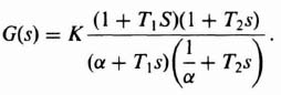
   Find the frequency ω₀ where the phase angle of G(jω) becomes zero. For frequencies less than ω₀, this network acts as a phase-lag network; for frequencies greater than ω₀, this network acts as a phase-lead network.

8. 2.8. It is desired that a unity feedback control system whose forward transfer function is G(s) = 20/[s(1 + 0.2s)(1 + 0.5s)] have a minimum phase margin of 45° and a minimum gain margin of 20 dB.
   1. Specify the time constant of a phase-lead network (or networks) that can achieve this.
   2. Repeat part (a) for a phase-lag network.
9. 2.9. It is desired that a unity feedback control system whose forward transfer function is G(s) = 20/[s(1 + 0.5s)(1 + 00.001s)] have a phase margin of 60° and a gain margin of 60 dB. Determine the time constants of a phase-lag network (or networks) that can achieve this.
10. 2.10. The temperature-control loop of a nuclear power plant is illustrated in Figure P2.10. The transfer function of the nuclear reactor can be adequately represented by

    

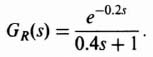
    A time delay (or transportation lag) is included in this transfer function to account for the time required to transport the fluid from the reactor to the measurement point. A proportional-plus-integral (PI) controller is used for compensation.

    

    Figure P2.10

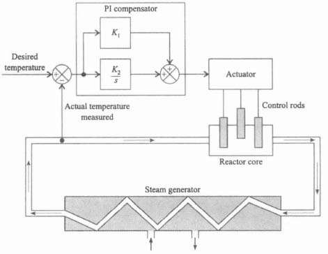
    Using the Bode diagram, determine the values of K₁ and K₂ in order to achieve a phase margin of 30° and a gain margin of 4 dB.

11. 2.11. It is desired that a unity feedback control system whose forward transfer function is G(s) = 1.5/[s²(0.1s + 1)] have a phase margin of 45° at the crossover frequency. Determine the stabilizing element required to achieve this.
12. 2.12. It is desired that a unity feedback control system whose forward transfer function is G(s) = 0.15/[s²(0.1s + 1)] have a phase margin of 45° at the crossover frequency. Determine the stabilizing element required to achieve this.
13. 2.13. The H.S. Denison, shown in Figure P2.13a, the first large hydrofoil seacraft built and operated in the United States [13] was designed and built by the Grumman Aerospace Corporation for the Maritime Administration of the U.S. Department of Commerce. The 80-ton hydrofoil is capable of operating at speeds of 60 knots in seas containing waves nine feet high. A simplified schematic of the automatic control system of the H.S. Denison is illustrated in Figure P2.13b. It consists of transducers for sensing craft motions and a computer for transmitting commands to the electrohydraulic actuators [13]. Heave rate is fed symmetrically to the forward flaps; roll and roll rate are fed differentially to the forward flaps; pitch rate is fed to the stern foil. The stabilization control system maintains level flight by means of two main surface piercing foils located ahead of the center of gravity and an all-movable submerged foil aft. An equivalent block diagram of the pitch-control system is illustrated in Figure 2.13c. It is desired that the craft maintain a constant level of travel despite a wave disturbance U(s) whose energy is concentrated at 1 rad/sec. Assume that the specifications require that the pitch loop maintain a gain of 40 dB at 1 rad/sec in order to minimize the wave disturbance, and a crossover of 10 rad/sec for adequate response time. In addition, it is desired to have a phase margin of at least 50° at the gain crossover frequency of 10 rad/sec and a gain margin of 12 dB. Select the amplifier gain K_a and compensation network G_c(s) in order to achieve these requirements.

    

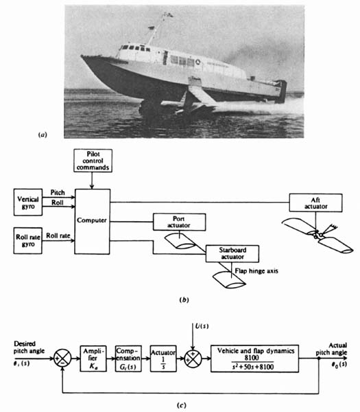
    Figure P2.13 (a) Photograph of H. S. Denison. (Courtesy of Grumman Aerospace Corporation) (b) The automatic control system. (c) Block diagram of the pitch-control system.

14. 2.14. It is desired that a unity feedback control system who se forward transfer function is G(s) = 99/[(1 + 0.1s)(1 + 0.2s)(1 + 1.5s)] have a phase margin of 45° at the gain crossover frequency. Determine the compensation required and the resulting gain crossover frequency to meet this specification.
15. 2.15. A unity-feedback control system has a forward transfer function given by

    

    1. Determine the gain crossover frequency and the phase margin of this control system.
    2. A phase-lead network, as defined in Eq. (2.6), is to be added in cascade with G₀(s) so that the phase margin is 70°. Determine the phase-lead network which will achieve this phase margin.
16. 2.16. A remotely piloted aircraft (RPA) for reconnaissance purposes over heavily defended terrain is to be controlled from a ground station. Use of the RPA will eliminate loss of human life if the aircraft is destroyed due to enemy action. The conceptual diagram of the RPA system is illustrated in Figure P2.16a.

    An equivalent block diagram of the pitch attitude axis of the RPA system is illustrated in Figure P2.16b.

    The transportation lag T₁ represents the delay caused by the man-in-the-loop at the ground station and the time it takes to transmit the signal from the ground station to the RPA. The transportation lag T₂ represents the time it takes for the return signal to be received by the ground station from the RPA. Assume that T₁ = 0.3 sec and that T₂ = 0.05 sec.

    1. Determine analytically the gain crossover frequency needed to achieve a phase margin of 50°.

       

       Figure P2.16

    2. Without drawing a Bode diagram, determine the value of K needed to obtain the gain crossover frequency obtained in part (a).
17. 2.17. Space vehicles, such as the space shuttle, using wings to maneuver while reentering the Earth's atmosphere present an interesting control problem.

    

    Figure P2.17

    Figure P2.17a illustrates a conceptual design of such a system and Figure P2.17b indicates the block diagram of its pitch-rate control system [14].

    1. Draw the Bode diagram of this system with K₁, = 1 and K₂ = 0. What are the resulting gain and phase margins?
    2. Select the values of K₁ and K₂ which will result in a gain crossover frequency of 1 rad/sec, a phase margin of at least 30° and a gain margin of at least 16 dB.
18. 2.18. It is desired that a unity feedback control system whose forward transfer function is G(s) = 20/[s(1 + s)(1 + 0.1s)] have a phase margin of 55° at the gain crossover frequency, and a gain margin of 25 dB. Determine a phase-lend network (s) and the resulting gain crossover frequency to meet this specification.
19. 2.19. The design of the Lunar Excursion Module (LEM) shown in Figure P2.19a, was an extremely interesting problem [15]. The control, guidance, and navigation for the LEM are provided by an all-digital system from the sensors to the gas-jet propulsion units. For purposes of this analysis, the vehicle dynamics can be approximated by a double integration, as indicated in Figure P2.19b, which illustrates one axis of the attitude-control system. In addition, the torque T(s) is assumed to be proportional to the control signal U(s). Assume that J = 0.25 and

    

    Utilizing the Bode diagram for solution, determine a lead-compensation network G_c(s) which will result in a crossover frequency of 5.1 rad/sec and a phase margin of 60°.

20. 2.20. It is desired to add cascade compensation to a unity feedback control system whose forward transfer function is G(s) = 60(1 + 0.5s)/[s(1 + 5s)] in order that the peak overshoot to a step input be approximately 12%.
    1. Using the Nichols chart, design a phase-lead network which can achieve this.
    2. With the compensation network chosen in part (a), determine the closed-loop amplitude and phase-frequency response.
21. 2.21. It is desired to add cascade compensation to a unity feedback control system whose forward transfer function is G(s) = 19.1/[s(1 + s)(1 + 0.1s)] in order that M_p = 0.75 while the same steady-state error is maintained.
    1. Design a phase-lead network to achieve this.
    2. With the compensation network chosen in part (a), determine the closed-loop amplitude and phase frequency response.

    

    Figure P2.19

22. 2.22. It is desired that the system considered in Problem 2.21 have a peak overshoot of approximately 15% to a step input.
    1. Utilizing a minor rate-feedback loop, specify the tachometer constant which can achieve this.
    2. What will be the resulting system steady-state error to a unit ramp input with the minor rate-feedback loop added?
    3. Utilizing a simple high-pass RC filter in cascade with the tachometer, determine the time constant of the network and the tachometer constant which will result in a 15% overshoot to a step input.
    4. What will be the steady-state error to a unit ramp when the high-pass filter is cascaded with the tachometer?
23. 2.23. It is desired that a unity feedback control system whose forward transfer function is G(s) = K/[s(1 + 0.1s)(1 + s)] have a damping ratio of 0.75 for the dominant complex roots. Using the root-locus method, determine the increase in gain and phase-lag network (s + nα)/(s + α) which can achieve this. Assume K_ν = 15.
24. 2.24. A unity-feedback control system has a forward transfer function given by:

    

    1. Draw the Bode diagram of this control system and determine the resulting phase margin and gain margin.
    2. To achieve an acceptable transient response for this system, the phase margin should be approximately 30° and the gain margin 20 dB. In addition, a sinusoidal disturbance is present at 0.1 rad/sec, and a gain of 60 dB is required at this frequency to nullify its effect. Design a passive compensation network which will achieve the desired transient response and accuracy, and also minimize the noise susceptibility of the system.
25. 2.25. The block diagram of one axis of a robotic positioning system that uses rate feedback for compensation is illustrated in Figure P2.25.

    

    Figure P2.25

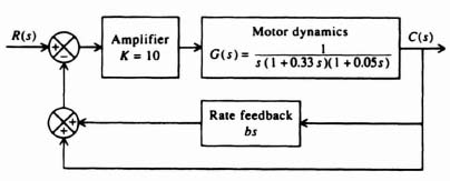
    1. Without any rate feedback (b = 0), determine the gain crossover frequency, phase margin and gain margin of the uncompensated system using the Bode-diagram method.
    2. For proper operation of the robot, a minimum phase margin of 65° and a minimum gain margin of 90 dB are desired. Using the Bode diagram, determine the amount of rate-feedback constant b which will achieve these requirements.
26. 2.26. The system shown in Figure P2.26 contains a proportional plus integral (PI) controller. The PI controller contains a zero term at s = −K and a pole at s = 0. Therefore, the PI controller has infinite gain at zero frequency, and it behaves as a phase-lag network. This feature improves the steady-state characteristics.

    

    Figure P2.26

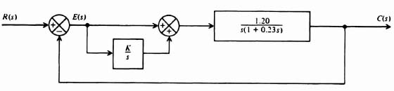
    1. Determine the steady-state error of this system to a unit step input.
    2. Determine the steady-state error of this system to a unit ramp input.
    3. Determine the range of gain K for which this system is stable.
27. 2.27. A negative-feedback system containing unity feedback has a forward transfer function given by

    

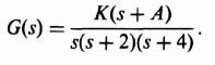
    The zero factor (s + A) in the numerator of this transfer is to be used to compensate the system. Utilizing the root locus, analyze the effects on system stability of the following values of A:

    

    What conclusions can you draw from your results on the best value of A for compensating this system? What happens if A is greater than 6?

28. 2.28. A unity-feedback control system has a forward transfer function given by:

    

    We wish to use a proportional plus integral (PI) controller in cascade with G₀(s) to compensate this control system. The transfer function of this compensator is given by:

    

    Select K so that the pair of dominant closed-loop poles for this control system is located at s = −0.5 ± 0.5j.

29. 2.29. A unity-feedback control system has the following forward transfer function:

    

    Determine the values of α so that the root locus will have zero breakaway points, not including the one at s equal zero.

30. 2.30. The forward transfer function of a unity-feedback control system is given by the following:

    

    1. Construct the root-locus diagram for 0 ≤ K ≤ ∞, and show all pertinent values on the root locus. What conclusions can you reach from this root-locus diagram?
    2. The system will be stabilized by means of a rate-feedback element (e.g., tachometer) added in parallel to the unity feedback so that the total feedback transfer function becomes:

       

       Construct the root locus of this compensated control system for 0 ≤ K ≤ ∞, and show all pertinent values on the root locus.

31. 2.31. The transfer functions of a negative feedback system are given by the following:

    

    1. Sketch the root locus.
    2. Determine C(s)/R(s), with the denominator in factored form, if a damping ratio of 0.5 is required for the dominant roots.
32. 2.32. Determine the increase in gain and phase-lag network compensation required to stabilize a unity-feedback system whose forward transfer function is given by

    

    The requirement for the system damping ratio is 0.707, and the velocity constant is 100/sec.

33. 2.33. A unity-feedback control system has a forward transfer function given by

    

    It is desired that the system have a velocity constant of 15 and a damping ratio of 0.75. Using the root-locus method, determine the increase in gain and phase-lag network (s + nα)/(s + α) which can achieve this, assuming that the transient response is governed by a pair of dominant complex-conjugate poles.

34. 2.34. A unity-feedback control system has a forward transfer function given by

    

    It is desired that the system have a velocity constant of 150 and a damping ratio of 0.75. Using the root-locus method, determine the increase in gain and phase-lag network, represented by (s + nα)/(s + α), which can achieve this. Assume that the transient response is governed by a pair of dominant complex-conjugate poles. Show all pertinent points on the root locus before and after compensation.

35. 2.35. The block diagram of a positioning system is shown in Figure P2.35.

    

    Figure P2.35

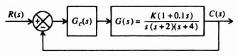
    1. Without any compensation, G_c(s) = 1, draw the root locus of the uncompensated system. On this diagram determine and show the following clearly:
       • Point (s) of breakaway from the real axis
       • Crossing (s) of the imaginary axis
       • K_max
       • All asymptotes.
    2. It is desired that the system have a velocity constant of 4 and a damping ratio of 0.707. Using the root-locus method, determine the compensation G_c(s) which can achieve this. Assume that the transient response is governed by a pair of dominant complex-conjugate poles. Show all pertinent changes and points on the root locus after compensation. (An exact recalculation of the point (s) of breakaway, the crossing of the imaginary axis, and K_max are not necessary.)
36. 2.36. In order to obtain a control system which has an infinite velocity constant, a control-system engineer designs the control system of Figure P2.36, which he or she recognizes will need some compensation network, G_c(s).

    

    Figure P2.36

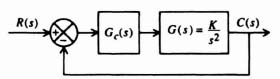
    1. Without any compensation, G_c(s) = 1, draw the root locus of this control system. From a practical viewpoint, is it stable?
    2. The control-system engineer desires to use a passive compensation network for G_c(s), either a phase-lag or a phase-lead network. Assume that the resistors and capacitors that are available can provide a zero at −1 and a pole at −2, or a pole at −1 and a zero at −2. As the control-system engineer, which would you select and why? Draw the root locus for your stabilized control system (with either a phase-lag or a phase-lead network). Show all pertinent points on your root locus.
37. 2.37. The signal-flow graph of the temperature-control loop for a xylene chemical process [16] is shown in Figure P2.37. The temperature of the process, C(s), is related to the heat supplied to the process by the quadratic transfer function G_p(s). Temperature is measured by a sensor having a pole at s = −0.3, and the output of the sensor in the form of air pressure is compared with the desired value of temperature as indicated by the reference pressure R(s). The pressure difference (a measure of temperature error) actuates a pneumatic controller which provides as its output a pneumatic actuating signal applied to a steam valve. The valve, in turn, controls the flow of heat to the xylene column in order to minimize the error.

    

    Figure P2.37

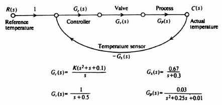
    1. Draw the root locus for this system.
    2. Determine the required gain K for a damping ratio of 0.5.
38. 2.38. It is desired that a unity feedback control system whose forward transfer function is G(s) = K(1 + s)/[s²(1 + 0.1s)] have a damping ratio of 0.75 for the dominant complex roots. Using the root-locus method, determine the value of K which can achieve this.
39. 2.39. A turbine speed-control system is illustrated in Figure P2.39. Assume that the transfer function of the control valve, turbine, and speed converter are:

    

    

    Figure P2.39

    Assuming that the transient response is governed by a pair of dominant complex-conjugate poles, determine the value of the controller gain K in order that the system has a damping ratio of 0.5.

40. 2.40. It is desired that a unity feedback control system whose forward transfer function is G(s) = K(s + 1)/[s(s² + 8s + 16)] have a damping ratio of 0.75 for the dominant complex roots. Using the root-locus method:
    1. Determine the value of K which can achieve this.
    2. Determine the values of ω_p and M_p for the value of K found in part (a) using the Nichols chart.
41. 2.41. Determine the gain needed for a unity feedback control system whose forward transfer function is G(s) = K(s + 0.1)²/[s²(s² + 9s + 20)] which can achieve a damping ratio of 0.75.
42. 2.42. Unlike fixed-wing aircraft, which possess a moderate degree of inherent stability, the helicopter is very unstable and requires the use of feedback loops for stabilization. A typical control system involves the use of an inner automatic stabilization loop and an outer loop which is controlled by the pilot, who inserts commands into it based on attitude errors displayed to the pilot.

    

    Figure P2.43

    Figure P2.42 illustrates the pitch-control system used on the S-55 helicopter [17]. When the pilot is not utilizing the control stick, the switch S₁ is open, which disengages the pilot control loop. The model of the pilot's transfer function, G₁(s), includes a gain factor, an anticipation time constant of 1 sec, and an error-smoothing time constant of 10 sec [17].

    1. With the pilot control loop open, plot the root locus for the automatic stabilization loop and determine the gain K₂ which results in a damping ratio of 0.5 for the dominant complex roots.
    2. Draw the root locus of the pilot control loop with K₂ set at the value determined in part (a). Determine the value of the pilot's gain compensation factor K₁ in order that the pilot control loop have a damping ratio of 0.5.
43. 2.43. Many modern control systems are designed to be adaptive, in order that they can achieve a desired response in the presence of extreme changes in the system parameters and major external disturbances. Adaptive control systems are usually characterized by devices that automatically measure the dynamics of the controlled system and by other devices that automatically adjust the characteristics of the controlled elements based on a comparison of the measurements with some optimum figure of merit. Figure P2.43 illustrates an adaptive pitch flight control system [18]. It attempts to measure the exact location of a pair of dominant, variable, servo actuator poles that move in the complex plane, as a function of the flight conditions. The adaptive feature overcomes this problem by adjusting the gain in order to keep the location of these sensitive poles fixed in the complex plane. A test impulse train is injected into the system when the error is small. The performance computer determines the transient response of the system and compares it with an optimum desired response that is set at 2 half cycles of a transient response over a 3-sec interval of time. The performance computer is designed so that a count less than 2 over a 3-sec period will cause the adaptor motor to increase K, and a count greater than 2 over a 3-sec period will cause the adaptor motor to decrease K. Assume that the poles and zeros of the system are located in the complex plane as follows:

    Table P2.43. Helicopter Control System Parameters

    

    1. Draw the root locus of this system.
    2. Determine the variable gain K that will result in a damping ratio of 0.3, assuming that the transient response is governed by a pair of dominant complex-conjugate poles.
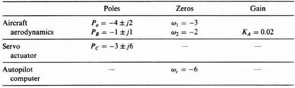
44. 2.44. Repeat Problem 2.33 for

    

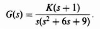
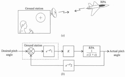
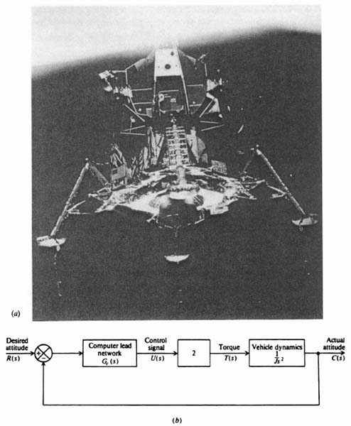
REFERENCES

1. W. R. Ahrendt, Servomechanism Practice. McGraw-Hill, New York, 1954.

2. J. G. Truxal, Automatic Feedback Control System Synthesis. McGraw-Hill, New York, 1955.

3. R. E. Kalman, “On the general theory of control systems.” In Proceedings of the First International Congress of Automatic Control, Moscow, 1960.

4. R. E. Kalman, Y. C. Ho, and K. S. Navendra, “Controllability of linear dynamical systems,” Contrib. Diff. Equat., 1, 189–213 (1961).

5. H. Lauer, R. N., Lesnick, and L. E. Matson, Servomechanism Fundamentals. McGraw-Hill, New York, 1960.

6. J. G. Truxal, ed. Control Engineer's Handbook. McGraw-Hill, New York, 1955.

7. H. W. Bode, Network Analysis and Feedback Amplifier Design. Van Nostrand, New York, 1945.

8. L. A. Gould, Chemical Process Control: Theory and Applications. Addison-Wesley, Reading, MA, 1969.

9. H. Chestnut and R. W. Mayer, Servomechanisms and Regulating System Design, 2nd ed., Vol. 1, Wiley, New York, 1959.

10. J. L. Bower and P. M. Schultheiss, Introduction to the Design of Servomechanisms. Wiley, New York, 1958.

11. S. M. Shinners, “How to approach the stability analysis and compensation of control systems.” Control Eng. 25(5), 62–67 (1978).

12. W. K. Waymeyer and R. W. Sporing, “Closed loop adaptation applied to missile control,” In Proceedings of the 1962 Joint Automatic Control Conference. New York, p. 18–33.

13. R. M. Rose, The Rough Water Performance of the H. S. Denison, Paper No. 64–197. Am. Inst. Aeronaut. Astronaut., Washington, DC, 1984.

14. R. P. Kotfile and S. S. Oseder, “Stabilization and control of maneuvering reentry vehicle.” Sperry Eng. Rev. 18, 2–10 (1965).

15. F. Doennebrink and J. Russel, “LEM stabilization and control system.” AIAA/ION Guidance and Control Conference. 1965, pp. 430–441.

16. W. A. Lynch and J. G. Truxal, Principles of Electronic Instrumentation. McGraw-Hill, New York, 1962.

17. L. Kaufman, “Helicopter control stick steering,” Sperry Eng. Rev. 11, 41–48 (1958).

18. F. C. Gregory, ed. Proceedings of the Self-Adaptive Flight Control Systems Symposium, WADC Techn. Rep. No. 59–49, ASTIA Doc. No. AD 209389, 1959.

19. S. M. Shinners, Techniques of System Engineering. McGraw-Hill, New York, 1967.