CHAPTER TWENTY-TWO
Network Flow

GRAPHS, DIGRAPHS, AND networks are just mathematical abstractions, but they are useful in practice because they help us to solve numerous important problems. In this chapter, we extend the network problem-solving model to encompass a dynamic situation where we imagine material flowing through the network, with different costs attached to different routes. These extensions allow us to tackle a surprisingly broad variety of problems with a long list of applications.

We see that these problems and applications can be handled within a few natural models that we can relate to one another through reduction. There are several different ways, all of which are technically equivalent, to formulate the basic problems. To implement algorithms that solve them all, we settle on two specific problems, develop efficient algorithms to solve them, then develop algorithms that solve other problems by finding reductions to the known problems.

In real life, we do not always have the freedom of choice that this idealized scenario suggests, because not all pairs of reduction relationships between these problems have been proved, and because few optimal algorithms for solving any of the problems are known. Perhaps no efficient direct solution to a given problem has yet been invented, and perhaps no efficient reduction that directly relates a given pair of problems has yet been devised. The network-flow formulation that we cover in this chapter has been successful not only because simple reductions to it are easy to define for many problems, but also because numerous efficient algorithms for solving the basic network-flow problems have been devised.

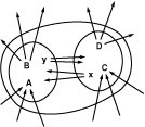
Figure 22.1 Distribution problem

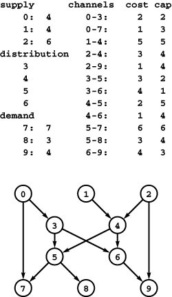
In this instance of the distribution problem, we have three supply vertices (0 through 2), four distribution points (3 through 6), three demand vertices (7 through 9), and twelve channels. Each supply vertex has a rate of production; each demand vertex a rate of consumption; and each channel a maximum capacity and a cost per unit distributed. The problem is to minimize costs while distributing material through the channels (without exceeding capacity anywhere) such that the total rate of material leaving each supply vertex equals its rate of production; the total rate at which material arrives at each demand vertex equals its rate of consumption; and the total rate at which material arrives at each distribution point equals the total rate at which material leaves.

The following examples illustrate the range of problems that we can handle with network-flow models, algorithms, and implementations. They fall into general categories known as distribution problems, matching problems, and cut problems, each of which we examine in turn. We indicate several different related problems, rather than lay out specific details in these examples. Later in the chapter, when we undertake to develop and implement algorithms, we give rigorous descriptions of many of the problems mentioned here.

In distribution problems, we are concerned with moving objects from one place to another within a network. Whether we are distributing hamburger and chicken to fast-food outlets or toys and clothes to discount stores along highways throughout the country—or software to computers or bits to display screens along communications networks throughout the world—the essential problems are the same. Distribution problems typify the challenges that we face in managing a large and complex operation. Algorithms to solve them are broadly applicable and are critical in numerous applications.

Merchandise distribution A company has factories, where goods are produced; distribution centers, where the goods are stored temporarily; and retail outlets, where the goods are sold. The company must distribute the goods from factories through distribution centers to retail outlets on a regular basis, using distribution channels that have varying capacities and unit distribution costs. Is it possible to get the goods from the warehouses to the retail outlets such that supply meets demand everywhere? What is the least-cost way to do so? Program 22.1 illustrates a distribution problem.

Figure 22.2 illustrates the transportation problem, a special case of the merchandise-distribution problem where we eliminate the distribution centers and the capacities on the channels. This version is important in its own right and is significant (as we see in Section 22.7) not just because of important direct applications but also because it turns out not to be a “special case” at all—indeed, it is equivalent in difficulty to the general version of the problem.

Communications A communications network has a set of requests to transmit messages between servers that are connected by channels (abstract wires) that are capable of transferring information at varying rates. What is the maximum rate at which information can be transferred between two specified servers in the network? If there are costs associated with the channels, what is the cheapest way to send the information at a given rate that is less than the maximum?

Figure 22.2 Transportation problem

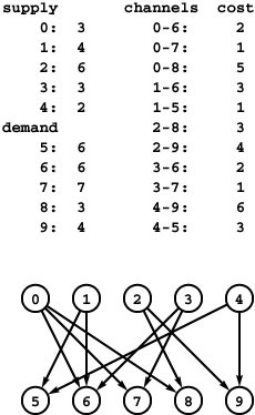
The transportation problem is like the distribution problem, but with no channel-capacity restrictions and no distribution points. In this instance, we have five supply vertices (0 through 4), five demand vertices (5 through 9), and twelve channels. The problem is to find the lowest-cost way to distribute material through the channels such that supply exactly meets demand everywhere. Specifically, we require an assignment of weights (distribution rates) to the edges such that the sum of weights on outgoing edges equals the supply at each supply vertex; the sum of weights on ingoing edges equals the demand at each demand vertex; and the total cost (sum of weight times cost for all edges) is minimized over all such assignments.

Traffic flow A city government needs to formulate a plan for evacuating people from the city in an emergency. What is the minimum amount of time that it would take to evacuate the city, if we suppose that we can control traffic flow so as to realize the minimum? Traffic planners also might formulate questions like this when deciding which new roads, bridges, or tunnels might alleviate rush-hour or vacation-weekend traffic problems.

In matching problems, the network represents the possible ways to connect pairs of vertices, and our goal is to choose among the connections (according to a specified criterion) without including any vertex twice. In other words, the chosen set of edges defines a way to pair vertices with one another. We might be matching students to colleges, applicants to jobs, courses to available hours for a school, or members of Congress to committee assignments. In each of these situations, we might imagine a variety of criteria defining the characteristics of the matches sought.

Job placement A job-placement service arranges interviews for a set of students with a set of companies; these interviews result in a set of job offers. Assuming that an interview followed by a job offer represents mutual interest in the student taking a job at the company, it is in everyone’s best interests to maximize the number of job placements. Program 22.3 is an example illustrating that this task can be complicated.

Minimum-distance point matching Given two sets of N points, find the set of N line segments, each with one endpoint from each of the point sets, with minimum total length. One application of this purely geometric problem is in radar tracking systems. Each sweep of the radar gives a set of points that represent planes. We assume that the planes are kept sufficiently well spaced that solving this problem allows us to associate each plane’s position on one sweep to its position on the next, thus giving us the paths of all the planes. Other data-sampling applications can be cast in this framework.

In cut problems, such as the one illustrated in Program 22.4, we remove edges to cut networks into two or more pieces. Cut problems are directly related to fundamental questions of graph connectivity that we first examined in Chapter 18. In this chapter, we discuss a central theorem that demonstrates a surprising connection between cut and flow problems, substantially expanding the reach of network-flow algorithms.

Figure 22.3 Job placement

Suppose that we have six students, each needing jobs, and six companies, each needing to hire a student. These two lists (one sorted by student, the other sorted by company) give a list of job offers, which indicate mutual interest in matching students and jobs. Is there some way to match students to jobs so that every job is filled and every student gets a job? If not, what is the maximum number of jobs that can be filled?

Network reliability A simplified model considers a telephone network as consisting of a set of wires that connect telephones through switches such that there is the possibility of a switched path through trunk lines connecting any two given telephones. What is the maximum number of trunk lines that could be cut without any pair of switches being disconnected?

Cutting supply lines A country at war moves supplies from depots to troops along an interconnected highway system. An enemy can cut off the troops from the supplies by bombing roads, with the number of bombs required to destroy a road proportional to that road’s width. What is the minimum number of bombs that the enemy must drop to ensure that no troops can get supplies?

Each of the applications just cited immediately suggests numerous related questions, and there are still other related models, such as the job-scheduling problems that we considered in Chapter 21. We consider further examples throughout this chapter, yet still treat only a small fraction of the important, directly related practical problems.

The network-flow model that we consider in this chapter is important not just because it provides us with two simply stated problems to which many of the practical problems reduce but also because we have efficient algorithms for solving the two problems. This breadth of applicability has led to the development of numerous algorithms and implementations. The solutions that we consider illustrate the tension between our quest for implementations of general applicability and our quest for efficient solutions to specific problems. The study of network-flow algorithms is fascinating because it brings us tantalizingly close to compact and elegant implementations that achieve both goals.

We consider two particular problems within the network-flow model: the maxflow problem and the mincost-flow problem. We see specific relationships among these problem-solving models, the shortest-path model of Chapter 21, the linear-programming (LP) model of Part 8, and numerous specific problem models including some of those just discussed.

Figure 22.4 Cutting supply lines

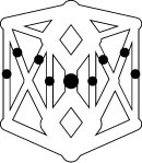
This diagram represents the roads connecting an army’s supply depot at the top to the troops at the bottom. The black dots represent an enemy bombing plan that would separate troops from supplies. The enemy’s goal is to minimize the cost of bombing (perhaps assuming that the cost of cutting an edge is proportional to its width), and the army’s goal is to design its road network to maximize the enemy’s minimum cost. The same model is useful in improving the reliability of communications networks and many other applications.

At first blush, many of these problems might seem to be completely different from network-flow problems. Determining a given problem’s relationship to known problems is often the most important step in developing a solution to that problem. Moreover, this step is often significant because, as is usual with graph algorithms, we must understand the fine line between trivial and intractable problems before we attempt to develop implementations. The infrastructure of problems and the relationships among the problems that we consider in this chapter provides a helpful context for addressing such issues.

In the rough categorization that we began with in Chapter 17, the algorithms that we examine in this chapter demonstrate that network-flow problems are “easy,” because we have straightforward implementations that are guaranteed to run in time proportional to a polynomial in the size of the network. Other implementations, although not guaranteed to run in polynomial time in the worst case, are compact and elegant and have been proved to solve a broad variety of other practical problems, such as the ones discussed here. We consider them in detail because of their utility. Researchers still seek faster algorithms, in order to enable huge applications and to save costs in critical ones. Ideal optimal algorithms that are guaranteed to be as fast as possible are yet to be discovered for network-flow problems.

On the one hand, some of the problems that we reduce to network-flow problems are known to be easier to solve with specialized algorithms. In principle, we might consider implementing and improving these specialized algorithms. Although that approach is productive in some situations, efficient algorithms for solving many of the problems (other than through reduction to network flow) are not known. Even when specialized algorithms are known, developing implementations that can outperform good network-flow codes can be a significant challenge. Moreover, researchers are still improving network-flow algorithms, and the possibility remains that a good network-flow algorithm might outperform known specialized methods for a given practical problem.

On the other hand, network-flow problems are special cases of the even more general LP problems that we discuss in Part 8. Although we could (and people often do) use an algorithm that solves LP problems to solve network-flow problems, the network-flow algorithms that we consider are simpler and more efficient than are those that solve LP problems. But researchers are still improving LP solvers, and the possibility remains that a good algorithm for LP problems might—when used for practical network-flow problems—outperform all the algorithms that we consider in this chapter.

The classical solutions to network-flow problems are closely related to the other graph algorithms that we have been examining, and we can write surprisingly concise programs that solve them, using the algorithmic tools we have developed. As we have seen in many other situations, good algorithms and data structures can achieve substantial reductions in running times. Development of better implementations of classical generic algorithms is still being studied, and new approaches continue to be discovered.

In Section 22.1 we consider basic properties of flow networks, where we interpret a network’s edge weights as capacities and consider properties of flows, which are a second set of edge weights that satisfy certain natural constraints. Next, we consider the maxflow problem, which is to compute a flow that is best in a specific technical sense. In Sections 22.2 and 22.3, we consider two approaches to solving the maxflow problem, and examine a variety of implementations. Many of the algorithms and data structures that we have considered are directly relevant to the development of efficient solutions of the maxflow problem. We do not yet have the best possible algorithms to solve the maxflow problem, but we consider specific useful implementations. In Section 22.4, to illustrate the reach of the maxflow problem, we consider different formulations, as well as other reductions involving other problems.

Maxflow algorithms and implementations prepare us to discuss an even more important and general model known as the mincost-flow problem, where we assign costs (another set of edge weights) and define flow costs, then look for a solution to the maxflow problem that is of minimal cost. We consider a classic generic solution to the mincost-flow problem known as the cycle-canceling algorithm; then, in Section 22.6, we give a particular implementation of the cycle-canceling algorithm known as the network simplex algorithm. In Section 22.7, we discuss reductions to the mincost-flow problem that encompass, among others, all the applications that we just outlined.

Network-flow algorithms are an appropriate topic to conclude this book for several reasons. They represent a payoff on our investment in learning basic algorithmic tools such as linked lists, priority queues, and general graph-search methods. The graph-processing classes that we have studied lead immediately to compact and efficient class implementations for network-flow problems. These implementations take us to a new level of problem-solving power and are immediately useful in numerous practical applications. Furthermore, studying their applicability and understanding their limitations sets the context for our examination of better algorithms and harder problems—the undertaking of Part 8.

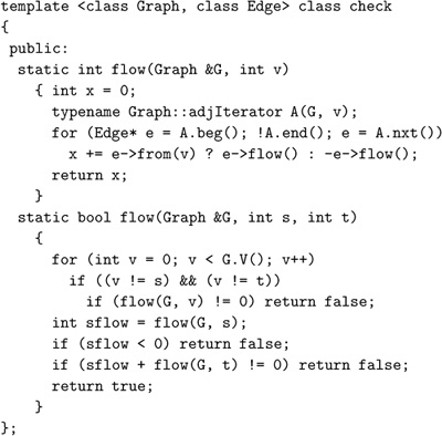
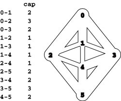
Figure 22.5 Network flow

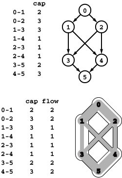
A flow network is a weighted network where we interpret edge weights as capacities (top). Our objective is to compute a second set of edge weights, bounded by the capacities, which we call the flow. The bottom drawing illustrates our conventions for drawing flow networks. Each edge’s width is proportional to its capacity; the amount of flow in each edge is shaded in gray; the flow is always directed down the page from a single source at the top to a single sink at the bottom; and intersections (such as 1-4 and 2-3 in this example) do not represent vertices unless labeled as such. Except for the source and the sink, flow in is equal to flow out at every vertex: For example, vertex 2 has 2 units of flow coming in (from 0) and 2 units of flow going out (1 unit to 3 and 1 unit to 4).

22.1 Flow Networks

To describe network-flow algorithms, we begin with an idealized physical model in which several of the basic concepts are intuitive. Specifically, we imagine a collection of interconnected oil pipes of varying sizes, with switches controlling the direction of flow at junctions, as in the example illustrated in Program 22.5. We suppose further that the network has a single source (say, an oil field) and a single sink (say, a large refinery) to which all the pipes ultimately connect. At each vertex, the flowing oil reaches an equilibrium where the amount of oil flowing in is equal to the amount flowing out. We measure both flow and pipe capacity in the same units (say, gallons per second).

If every switch has the property that the total capacity of the ingoing pipes is equal to the total capacity of the outgoing pipes, then there is no problem to solve: We simply fill all pipes to full capacity. Otherwise, not all pipes are full, but oil flows through the network, controlled by switch settings at the junctions, such that the amount of oil flowing into each junction is equal to the amount of oil flowing out. But this local equilibrium at the junctions implies an equilibrium in the network as a whole: We prove in Property 22.1 that the amount of oil flowing into the sink is equal to the amount flowing out of the source. Moreover, as illustrated in Program 22.6, the switch settings at the junctions of this amount of flow from source to sink have nontrivial effects on the flow through the network. Given these facts, we are interested in the following question: What switch settings will maximize the amount of oil flowing from source to sink?

We can model this situation directly with a network (a weighted digraph, as defined in Chapter 21) that has a single source and a single sink. The edges in the network correspond to the oil pipes, the vertices correspond to the junctions with switches that control how much oil goes into each outgoing edge, and the weights on the edges correspond to the capacity of the pipes. We assume that the edges are directed, specifying that oil can flow in only one direction in each pipe. Each pipe has a certain amount of flow, which is less than or equal to its capacity, and every vertex satisfies the equilibrium condition that the flow in is equal to the flow out.

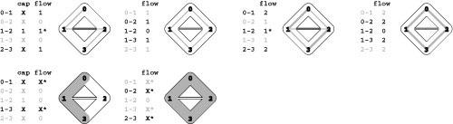
Figure 22.6 Controlling flow in a network

We might initialize the flow in this network by opening the switches along the path 0-1-3-5, which can handle 2 units of flow (top), and by opening switches along the path 0-2-4-5 to get another 1 unit of flow in the network (center). Asterisks indicate full edges.

Since 0-1, 2-4, and 3-5 are full, there is no direct way to get more flow from 0 to 5, but if we change the switch at 1 to redirect enough flow to fill 1-4, we open up enough capacity in 3-5 to allow us to add flow on 0-2-3-5, giving a maxflow for this network (bottom).

This flow-network abstraction is a useful problem-solving model that applies directly to a variety of applications and indirectly to still more. We sometimes appeal to the idea of oil flowing through pipes for intuitive support of basic ideas, but our discussion applies equally well to goods moving through distribution channels and to numerous other situations.

The flow model directly applies to a distribution scenario: We interpret the flow values as rates of flow, so that a flow network describes the flow of goods in a manner precisely analogous to the flow of oil. For example, we can interpret the flow in Program 22.5 as specifying that we should be sending two items per time unit from 0 to 1 and from 0 to 2, one item per time unit from 1 to 3 and from 1 to 4, and so forth.

Another way to interpret the flow model for a distribution scenario is to interpret flow values as amounts of goods so that a flow network describes a one-time transfer of goods. For example, we can interpret the flow in Program 22.5 as describing the transfer of four items from 0 to 5 in the following three-step process: First, send two items from 0 to 1 and two items from 0 to 2, leaving two items at each of those vertices. Second, send one item each from 1 to 3, 1 to 4, 2 to 3, and 2 to 4, leaving two items each at 3 and 4. Third, complete the transfer by sending two items from 3 to 5 and two items from 4 to 5.

As with our use of distance in shortest-paths algorithms, we are free to abandon any physical intuition when convenient because all the definitions, properties, and algorithms that we consider are based entirely on an abstract model that does not necessarily obey physical laws. Indeed, a prime reason for our interest in the network-flow model is that it allows us to solve numerous other problems through reduction, as we see in Sections 22.4 and 22.6. Because of this broad applicability, it is worthwhile to consider precise statements of the terms and concepts that we have just informally introduced.

Definition 22.1 We refer to a network with a designated source s and a designated sink t as an st-network.

We use the modifier “designated” here to mean that s does not necessarily have to be a source (vertex with no incoming edges) and t does not necessarily have to be a sink (vertex with no outgoing edges), but that we nonetheless treat them as such, because our discussion (and our algorithms) will ignore edges directed into s and edges directed out of t. To avoid confusion, we use networks with a single source and a single sink in examples; we consider more general situations in Section 22.4. We refer to s and t as “the source” and “the sink,” respectively, in the st -network because those are the roles that they play in the network. We also refer to the other vertices in the network as the internal vertices.

Definition 22.2 A flow network is an st-network with positive edge weights, which we refer to as capacities. A flow in a flow network is a set of nonnegative edge weights—which we refer to as edge flows —satisfying the conditions that no edge’s flow is greater than that edge’s capacity and that the total flow into each internal vertex is equal to the total flow out of that vertex.

We refer to the total flow into a vertex (the sum of the flows on its incoming edges) as the vertex’s inflow and the total flow out of a vertex (the sum of the flows on its outgoing edges) as the vertex’s outflow. By convention, we set the flow on edges into the source and edges out of the sink to zero, and in Property 22.1 we prove that the source’s outflow is always equal to the sink’s inflow, which we refer to as the network’s value. With these definitions, the formal statement of our basic problem is straightforward.

Maximum flow Given an st -network, find a flow such that no other flow from s to t has larger value. For brevity, we refer to such a flow as a maxflow and the problem of finding one in a network as the maxflow problem. In some applications, we might be content to know just the maxflow value, but we generally want to know a flow (edge flow values) that achieves that value.

Variations on the problem immediately come to mind. Can we allow multiple sources and sinks? Should we be able to handle networks with no sources or sinks? Can we allow flow in either direction in the edges? Can we have capacity restrictions for the vertices instead of or in addition to the restrictions for the edges? As is typical with graph algorithms, separating restrictions that are trivial to handle from those that have profound implications can be a challenge. We investigate this challenge and give examples of reducing to maxflow a variety of problems that seem different in character, after we consider algorithms to solve the basic problem, in Sections 22.2 and 22.3.

Figure 22.7 Flow equilibrium

This diagram illustrates the preservation of flow equilibrium when we merge sets of vertices. The two smaller figures represent any two disjoint sets of vertices, and the letters represent flow in sets of edges as indicated: A is the amount of flow into the set on the left from outside the set on the right, x is the amount of flow into the set on the left from the set on the right, and so forth. Now, if we have flow equilibrium in the two sets, then we must have

A + x =B + y

for the set on the left and

C + y =D + x

for the set on the right. Adding these two equations and canceling the x + y terms, we conclude that

A + C =B + D,

or inflow is equal to outflow for the union of the two sets.

The characteristic property of flows is the local equilibrium condition that inflow be equal to outflow at each internal vertex. There is no such constraint on capacities; indeed, the imbalance between total capacity of incoming edges and total capacity of outgoing edges is what characterizes the maxflow problem. The equilibrium constraint has to hold at each and every internal vertex, and it turns out that this local property determines global movement through the network, as well. Although this idea is intuitive, it needs to be proved.

Property 22.1 Any st-flow has the property that outflow from s is equal to the inflow to t.

Proof: (We use the term st-flow to mean “flow in an st -network.”) Augment the network with an edge from a dummy vertex into s, with flow and capacity equal to the outflow from s, and with an edge from t to another dummy vertex, with flow and capacity equal to the inflow to t. Then, we can prove a more general property by induction: Inflow is equal to outflow for any set of vertices (not including the dummy vertices).

This property is true for any single vertex, by local equilibrium. Now, assume that it is true for a given set of vertices S and that we add a single vertex v to make the set S ^′=S {v}. To compute inflow and outflow for S ^′, note that each edge from v to some vertex in S reduces outflow (from v ) by the same amount as it reduces inflow (to S); each edge to v from some vertex in S reduces inflow (to v ) by the same amount as it reduces outflow (from S ); and all other edges provide inflow or outflow for S ^′ if and only if they do so for S or v. Thus, inflow and outflow are equal for S ^′, and the value of the flow is equal to the sum of the values of the flows of v and S minus sum of the flows on the edges connecting v to a vertex in S (in either direction).

Applying this property to the set of all the network’s vertices, we find that the source’s inflow from its associated dummy vertex (which

is equal to the source’s outflow) is equal to the sink’s outflow to its associated dummy vertex (which is equal to the sink’s inflow).

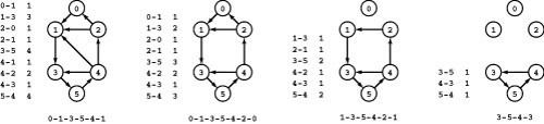
Figure 22.8 Cycle flow representation

This figure demonstrates that the circulation at left decomposes into the four cycles 1-3-5-4-1, 0-1-3-5-4-2-0, 1-3-5-4-2-1, 3-5-4-3, with weights 2, 1, 1, and 3, respectively. Each cycle’s edges appear in its respective column, and summing each edge’s weight from each cycle in which it appears (across its respective row) gives its weight in the circulation.

Corollary The value of the flow for the union of two sets of vertices is equal to the sum of the values of the flows for the two sets minus the sum of the weights of the edges that connect a vertex in one to a vertex in the other.

Proof: The proof just given for a set S and a vertex v still works if we replace v by a set T (which is disjoint from S ) in the proof. An example of this property is illustrated in Program 22.7.

We can dispense with the dummy vertices in the proof of Property 22.1, augment any flow network with an edge from t to s with flow and capacity equal to the network’s value, and know that inflow is equal to outflow for any set of nodes in the augmented network. Such a flow is called a circulation, and this construction demonstrates that the maxflow problem reduces to the problem of finding a circulation that maximizes the flow along a given edge. This formulation simplifies our discussion in some situations. For example, it leads to an interesting alternate representation of flows as a set of cycles, as illustrated in Program 22.8.

Given a set of cycles and a flow value for each cycle, it is easy to compute the corresponding circulation by following through each cycle and adding the indicated flow value to each edge. The converse property is more surprising: We can find a set of cycles (with a flow value for each) that is equivalent to any given circulation.

Property 22.2 (Flow decomposition theorem) Any circulation can be represented as flow along a set of at most E directed cycles.

Proof: A simple algorithm establishes this result. Iterate the following process as long as there is any edge that has flow: Starting with any

edge that has flow, follow any edge leaving that edge’s destination vertex that has flow and continue until encountering a vertex that has already been visited (a cycle has been detected). Go back around the cycle to find an edge with minimal flow; then reduce the flow on every edge in the cycle by that amount. Each iteration of this process reduces the flow on at least one edge to 0, so there are at most E cycles.

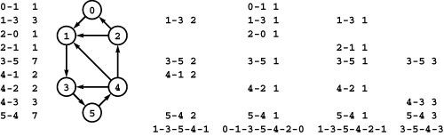
Figure 22.9 Cycle flow decomposition process

To decompose any circulation into a set of cycles, we iterate the following process: Follow any path until encountering a node for the second time, then find the minimum weight on the indicated cycle, then subtract that weight from each edge on the cycle and remove any edge whose weight becomes 0. For example, the first iteration is to follow the path 0-1-3-5-4-1 to find the cycle 1-3-5-4-1, then subtract 1 from the weights of each of the edges on the cycle, which causes us to remove 4-1 because its weight becomes 0. In the second iteration, we remove 0-1 and 2-0; in the third iteration, we remove 1-3, 4-2, and 2-1; and in the fourth iteration, we remove 3-5, 5-4, and 4-3.

Figure 22.9 illustrates the process described in the proof. For st-flows, applying this property to the circulation created by the addition of an edge from t to s gives the result that any st -flow can be represented as flow along a set of at most E directed paths, each of which is either a path from s to t or a cycle.

Corollary Any st-network has a maxflow such that the subgraph induced by nonzero flow values is acyclic.

Proof: Cycles that do not contain t-s do not contribute to the value of the flow, so we can change the flow to 0 along any such cycle without changing the value of the flow.

Corollary Any st-network has a maxflow that can be represented as flow along a set of at most E directed paths from s to t.

Proof: Immediate.

This representation provides a useful insight into the nature of flows that is helpful in the design and analysis of maxflow algorithms.

On the one hand, we might consider a more general formulation of the maxflow problem where we allow for multiple sources and sinks. Doing so would allow our algorithms to be used for a broader range of applications. On the other hand, we might consider special cases, such as restricting attention to acyclic networks. Doing so might make the problem easier to solve. In fact, as we see in Section 22.4, these variants are equivalent in difficulty to the version that we are considering. Therefore, in the first case, we can adapt our algorithms and implementations to the broader range of applications; in the second case, we cannot expect an easier solution. In our figures, we use acyclic networks because the examples are easier to understand when they have an implicit flow direction (down the page), but our implementations allow networks with cycles.

To implement maxflow algorithms, we use the GRAPH class of Chapter 20, but with pointers to a more sophisticated EDGE class. Instead of the single weight that we used in Chapters 20 and 21, we use pcap and pflow private data members (with cap() and flow() public member functions that return their values) for capacity and flow, respectively. Even though networks are directed graphs, our algorithms need to traverse edges in both directions, so we use the undirected graph representation from Chapter 20 and the member function from to distinguish u-v from v-u.

This approach allows us to separate the abstraction needed by our algorithms (edges going in both directions) from the client’s concrete data structure and leaves a simple goal for our algorithms: Assign values to the flow data members in the client’s edges that maximize flow through the network. Indeed, a critical component of our implementations involves a changing network abstraction that is dependent on flow values and implemented with EDGE member functions. We will consider an EDGE implementation (Program 22.2) in Section 22.2.

Since flow networks are typically sparse, we use an adjacency-lists-based GRAPH representation like the SparseMultiGRAPH implementation of Program 20.5. More important, typical flow networks may have multiple edges (of varying capacities) connecting two given vertices. This situation requires no special treatment with SparseMultiGRAPH, but with an adjacency-matrix–based representation, clients have to collapse such edges into a single edge.

In the network representations of Chapters 20 and 21, we used the convention that weights are real numbers between 0 and 1. In this chapter, we assume that the weights (capacities and flows) are all m-bit integers (between 0 and 2^m − 1). We do so for two primary reasons. First, we frequently need to test for equality among linear combinations of weights, and doing so can be inconvenient in floating-point representations. Second, the running times of our algorithms

can depend on the relative values of the weights, and the parameter M = 2^m gives us a convenient way to bound weight values. For example, the ratio of the largest weight to the smallest nonzero weight is less than M. The use of integer weights is but one of many possible alternatives (see, for example, Exercise 20.8) that we could choose to address these problems.

We sometimes refer to edges as having infinite capacity, or, equivalently, as being uncapacitated. That might mean that we do not compare flow against capacity for such edges, or we might use a sentinel value that is guaranteed to be larger than any flow value.

Figure 22.10 Flow network for exercises

This flow network is the subject of several exercises throughout the chapter.

Program 22.1 is an client function that checks whether a flow satisfies the equilibrium condition at every node and returns that flow’s value if the flow does. Typically, we might include a call to this function as the final action of a maxflow algorithm. Despite our confidence as mathematicians in Property 22.1, our paranoia as programmers dictates that we also check that the flow out of the source is equal to the flow into the sink. It might also be prudent to check that no edge’s flow exceeds that edge’s capacity and that the data structures are internally consistent (see Exercise 22.12).

Exercises

• 22.1 Find two different maxflows in the flow network shown in Program 22.10.

22.2 Under our assumption that capacities are positive integers less than M, what is the maximum possible flow value for any st-network with V vertices and E edges? Give two answers, depending on whether or not parallel edges are allowed.

• 22.3 Give an algorithm to solve the maxflow problem for the case that the network forms a tree if the sink is removed.

• 22.4 Give a family of networks with E edges having circulations where the process described in the proof of Property 22.2 produces E cycles.

22.5 Write an EDGE class that represents capacities and flows as real numbers between 0 and 1 that are expressed with d digits to the right of the decimal point, where d is a fixed constant.

• 22.6 Write a program that builds a flow network by reading edges (pairs of integers between 0 and V − 1) with integer capacities from standard input. Assume that the capacity upper bound M is less than 2²⁰.

22.7 Extend your solution to Exercise 22.6 to use symbolic names instead of integers to refer to vertices (see Program 17.10).

• 22.8 Find a large network online that you can use as a vehicle for testing flow algorithms on realistic data. Possibilities include transportation networks (road, rail, or air), communications networks (telephone or computer connections), or distribution networks. If capacities are not available, devise a reasonable model to add them. Write a program that uses the interface of Program 22.2 to implement flow networks from your data, perhaps using your solution to Exercise 22.7. If warranted, develop additional private functions to clean up the data, as described in Exercises 17.33–35.

22.9 Write a random-network generator for sparse networks with capacities between 0 and 2²⁰, based on Program 17.7. Use a separate class for capacities and develop two implementations: one that generates uniformly distributed capacities and another that generates capacities according to a Gaussian distribution. Implement client programs that generate random networks for both weight distributions with a well-chosen set values of V and E, so that you can use them to run empirical tests on graphs drawn from various distributions of edge weights.

22.10 Write a random-network generator for dense networks with capacities between 0 and 2²⁰, based on Program 17.8 and edge-capacity generators as described in Exercise 22.9. Write client programs to generate random networks for both weight distributions with a well-chosen set values of V and E, so that you can use them to run empirical tests on graphs drawn from these models.

• 22.11 Write a program that generates V random points in the plane, then builds a flow network with edges (in both directions) connecting all pairs of points within a given distance d of each other (see Program 3.20), setting each edge’s capacity using one of the random models described in Exercise 22.9. Determine how to set d so that the expected number of edges is E.

• 22.12 Modify Program 22.1 to also check that flow is less than capacity for all edges.

• 22.13 Find all the maxflows in the network depicted in Program 22.11. Give cycle representations for each of them.

22.14 Write a function that reads values and cycles (one per line, in the format illustrated in Program 22.8) and builds a network having the corresponding flow.

22.15 Write a client function that finds the cycle representation of a network’s flow using the method described in the proof of Property 22.2 and prints values and cycles (one per line, in the format illustrated in Program 22.8).

• 22.16 Write a function that removes cycles from a network’s st-flow.

• 22.17 Write a program that assigns integer flows to each edge in any given digraph that contains no sinks and no sources such that the digraph is a flow network that is a circulation.

• 22.18 Suppose that a flow represents goods to be transferred by trucks between cities, with the flow on edge u-v representing the amount to be taken from city u to v in a given day. Write a client function that prints out daily orders for truckers, telling them how much and where to pick up and how much and where to drop off. Assume that there are no limits on the supply of truckers and that nothing leaves a given distribution point until everything has arrived.

Figure 22.11 Flow network with cycle

This flow network is like the one depicted in Program 22.10, but with the direction of two of the edges reversed, so there are two cycles. It is also the subject of several exercises throughout the chapter.

22.2 Augmenting-Path Maxflow Algorithms

An effective approach to solving maxflow problems was developed by L. R. Ford and D. R. Fulkerson in 1962. It is a generic method for

Figure 22.12 Augmenting flow along a path

This sequence shows the process of increasing flow in a network along a path of forward and backward edges. Starting with the flow depicted at the left and reading from left to right, we increase the flow in 0-2 and then 2-3 (additional flow is shown in black). Then we decrease the flow in 1-3 (shown in white) and divert it to 1-4 and then 4-5, resulting in the flow at the right.

increasing flows incrementally along paths from source to sink that serves as the basis for a family of algorithms. It is known as the Ford– Fulkerson method in the classical literature; the more descriptive term augmenting-path method is also widely used.

Consider any directed path (not necessarily a simple one) from source to sink through an st -network. Let x be the minimum of the unused capacities of the edges on the path. We can increase the network’s flow value by at least x, by increasing the flow in all edges on the path by that amount. Iterating this action, we get a first attempt at computing flow in a network: Find another path, increase the flow along that path, and continue until all paths from source to sink have at least one full edge (so that we can no longer increase flow in this way). This algorithm will compute the maxflow in some cases, but will fall short in other cases. Program 22.6 illustrates a case where it fails.

To improve the algorithm such that it always finds a maxflow, we consider a more general way to increase the flow, along any path from source to sink through the network’s underlying undirected graph. The edges on any such path are either forward edges, which go with the flow (when we traverse the path from source to sink, we traverse the edge from its source vertex to its destination vertex) or backward edges, which go against the flow (when we traverse the path from source to sink, we traverse the edge from its destination vertex to its source vertex). Now, for any path with no full forward edges and no empty backward edges, we can increase the amount of flow in the network by increasing flow in forward edges and decreasing flow in backward edges. The amount by which the flow can be increased is limited by the minimum of the unused capacities in the forward edges and the flows in the backward edges. Program 22.12 depicts an example. In the new flow, at least one of the forward edges along the

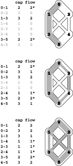
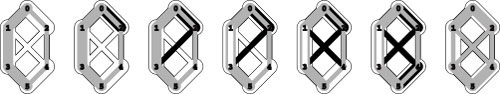
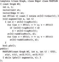
Figure 22.13 Augmenting-path sequences

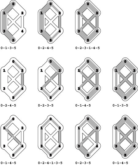
In these three examples, we augment a flow along different sequences of augmenting paths until no augmenting path can be found. The flow that results in each case is a maximum flow. The key classical theorem in the theory of network flows states that we get a maximum flow in any network, no matter what sequence of paths we use (see Property 22.5).

path becomes full or at least one of the backward edges along the path becomes empty.

The process just sketched is the basis for the classical Ford– Fulkerson maxflow algorithm (augmenting-path method). We summarize it as follows:

Remarkably, this method always finds a maxflow, no matter how we choose the paths. Like the MST method discussed in Section 20.1 and the Bellman–Ford shortest-paths method discussed in Section 21.7, itis a generic algorithm that is useful because it establishes the correctness of a whole family of more specific algorithms. We are free to use any method whatever to choose the path.

Figure 22.13 illustrates several different sequences of augmenting paths that all lead to a maxflow for a sample network. Later in this section, we examine several algorithms that compute sequences of augmenting paths, all of which lead to a maxflow. The algorithms differ in the number of augmenting paths they compute, the lengths of the paths, and the costs of finding each path, but they all implement the Ford–Fulkerson algorithm and find a maxflow.

To show that any flow computed by any implementation of the Ford–Fulkerson algorithm indeed has maximal value, we show that this fact is equivalent to a key fact known as the maxflow–mincut theorem. Understanding this theorem is a crucial step in understanding network-flow algorithms. As suggested by its name, the theorem is based on a direct relationship between flows and cuts in networks, so we begin by defining terms that relate to cuts.

Recall from Section 20.1 that a cut in a graph is a partition of the vertices into two disjoint sets, and a crossing edge is an edge that connects a vertex in one set to a vertex in the other set. For flow networks, we refine these definitions as follows (see Figure 22.14).

Definition 22.3 An st-cut is a cut that places vertex s in one of its sets and vertex t in the other.

Each crossing edge corresponding to an st-cut is either an st-edge that goes from a vertex in the set containing s to a vertex in the set containing t, or a ts -edge that goes in the other direction. We sometimes refer to the set of crossing edges as a cut set. The capacity of an st-cut in a flow network is the sum of the capacities of that cut’s st-edges, and the flow across an st-cut is the difference between the sum of the flows in that cut’s st -edges and the sum of the flows in that cut’s ts -edges.

Removing a cut set divides a connected graph into two connected components, leaving no path connecting any vertex in one to any vertex in the other. Removing all the edges in an st-cut of a network leaves no path connecting s to t in the underlying undirected graph, but adding any one of them back could create such a path.

Cuts are the appropriate abstraction for the application mentioned at the beginning of the chapter where a flow network describes the movement of supplies from a depot to the troops of an army. To cut off supplies completely and in the most economical manner, an enemy might solve the following problem.

Figure 22.14 st-cut terminology

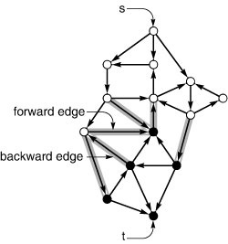
An st-network has one source s and one sink t. An st-cut is a partition of the vertices into a set containing s (white) and another set containing t (black). The edges that connect a vertex in one set with a vertex in the other (high-lighted in gray) are known as a cut set. A forward edge goes from a vertex in the set containing s to a vertex in the set containing t; a backward edge goes the other way. There are four forward edges and two backward edges in the cut set shown here.

Minimum cut Given an st-network, find an st-cut such that the capacity of no other cut is smaller. For brevity, we refer to such a cut as a mincut, and to the problem of finding one in a network as the mincut problem.

The mincut problem is a generalization of the connectivity problems that we discussed briefly in Section 18.6. We analyze specific relationships in detail in Section 22.4.

The statement of the mincut problem includes no mention of flows, and these definitions might seem to digress from our discussion of the augmenting-path algorithm. On the surface, computing a mincut (a set of edges) seems easier than computing a maxflow (an assignment of weights to all the edges). On the contrary, the key fact of this chapter is that the maxflow and mincut problems are intimately related. The augmenting-path method itself, in conjunction with two facts about flows and cuts, provides a proof.

Property 22.3 For any st-flow, the flow across each st-cut is equal to the value of the flow.

Proof: This property is an immediate consequence of the generalization of Property 22.1 that we discussed in the associated proof (see Figure 22.7). Add an edge t-s with flow equal to the value of the flow such that inflow is equal to outflow for any set of vertices. Then, for any st-cut where C _s is the vertex set containing s and C _t is the vertex set containing t, the inflow to C _s is the inflow to s (the value of the flow) plus the sum of the flows in the backward edges across the cut; and the outflow from C _s is the sum of the flows in the forward edges across the cut. Setting these two quantities equal establishes the desired result.

Property 22.4 No st-flow’s value can exceed the capacity of any st-cut.

Proof: The flow across a cut certainly cannot exceed that cut’s capacity, so this result is immediate from Property 22.3.

In other words, cuts represent bottlenecks in networks. In our military application, an enemy that is not able to cut off army troops

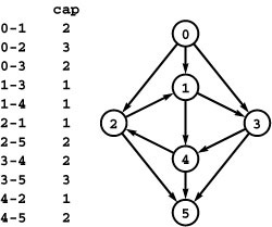
Figure 22.15 All st -cuts

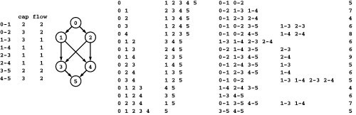
This list gives, for all the st-cuts of the network at left, the vertices in the set containing s, the vertices in the set containing t, forward edges, backward edges, and capacity (sum of capacities of the forward edges). For any flow, the flow across all the cuts (flow in forward edges minus flow in backward edges) is the same. For example, for the flow in the network at left, the flow across the cut separating 0 1 3 and 2 4 5 is 2 + 1 + 2 (the flow in 0-2, 1-4, and 3-5, respectively) minus 1 (the flow in 2-3), or 4. This calculation also results in the value 4 for every other cut in the network, and the flow is a maximum flow because its value is equal to the capacity of the minimum cut (see Property 22.5). There are two minimum cuts in this network.

completely from their supplies could still be sure that supply flow is restricted to at most the capacity of any given cut. We certainly might imagine that the cost of making a cut is proportional to its capacity in this application, thus motivating the invading army to find a solution to the mincut problem. More important, these facts also imply, in particular, that no flow can have value higher than the capacity of any minimum cut.

Property 22.5 (Maxflow–mincut theorem) The maximum value among all st-flows in a network is equal to the minimum capacity among all st-cuts.

Proof: It suffices to exhibit a flow and a cut such that the value of the flow is equal to the capacity of the cut. The flow has to be a maxflow because no other flow value can exceed the capacity of the cut and the cut has to be a minimum cut because no other cut capacity can be lower than the value of the flow (by Property 22.4). The Ford–Fulkerson algorithm gives precisely such a flow and cut: When the algorithm terminates, identify the first full forward or empty backward edge on every path from s to t in the graph. Let C _s be the set of all vertices that can be reached from s with an undirected path that does not contain a full forward or empty backward edge, and let C _t be the remaining vertices. Then, t must be in C _t, so (C_s, C_t)) is an st-cut, whose cut set consists entirely of full forward or empty backward edges. The flow across this cut is equal to the cut’s capacity (since forward edges are full and the backward edges are empty) and also to the value of the network flow (by Property 22.3).

This proof also establishes explicitly that the Ford–Fulkerson algorithm finds a maxflow. No matter what method we choose to find an augmenting path, and no matter what paths we find, we always end up with a cut whose flow is equal to its capacity, and therefore also is equal to the value of the network’s flow, which therefore must be a maxflow.

Another implication of the correctness of the Ford–Fulkerson algorithm is that, for any flow network with integer capacities, there exists a maxflow solution where the flows are all integers. Each augmenting path increases the flow by a positive integer (the minimum of the unused capacities in the forward edges and the flows in the backward edges, all of which are always positive integers). This fact justifies our decision to restrict our attention to integer capacities and flows. It is possible to design a maxflow with noninteger flows, even when capacities are all integers (see Exercise 22.23), but we do not need to consider such flows. This restriction is important: Generalizing to allow capacities and flows that are real numbers can lead to unpleasant anomalous situations. For example, the Ford–Fulkerson algorithm might lead to an infinite sequence of augmenting paths that does not even converge to the maxflow value (see reference section).

The generic Ford–Fulkerson algorithm does not specify any particular method for finding an augmenting path. Perhaps the most natural way to proceed is to use the generalized graph-search strategy of Section 18.8. To this end, we begin with the following definition.

Definition 22.4 Given a flow network and a flow, the residual network for the flow has the same vertices as the original and one or two edges in the residual network for each edge in the original, defined as follows: For each edge v-w in the original, let f be the flow and c the capacity. If f is positive, include an edge w-v in the residual with capacity f ; and if f is less than c, include an edge v-w in the residual with capacity c-f.

If v-w is empty (f is equal to 0), there is a single corresponding edge v-w with capacity c in the residual; if v-w is full (f is equal to c), there is a single corresponding edge w-v with capacity f in the residual; and if v-w is neither empty nor full, both v-w and w-v are in the residual with their respective capacities.

Program 22.2 defines the EDGE class that we use to implement the residual network abstraction with class function members. With such

Figure 22.16 Residual networks (augmenting paths)

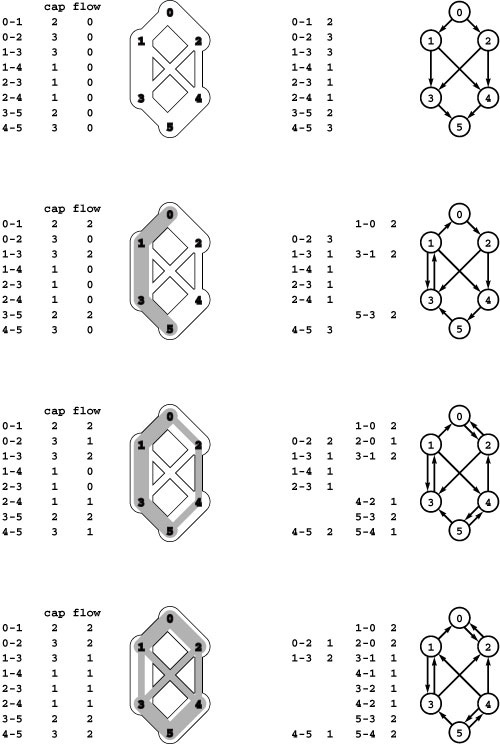
Finding augmenting paths in a flow network is equivalent to finding directed paths in the residual network that is defined by the flow. For each edge in the flow network, we create an edge in each direction in the residual network: one in the direction of the flow with weight equal to the unused capacity, and one in the opposite direction with weight equal to the flow. We do not include edges of weight 0 in either case. Initially (top), the residual network is the same as the flow network with weights equal to capacities. When we augment along the path 0-1-3-5 (second from top), we fill edges 0-1 and 3-5 to capacity so that they switch direction in the residual network, we reduce the weight of 1-3 to correspond to the remaining flow, and we add the edge 3-1 of weight 2. Similarly, when we augment along the path 0-2-4-5, we fill 2-4 to capacity so that it switches direction, and we have edges in either direction between 0 and 2 and between 4 and 5 to represent flow and unused capacity. After we augment along 0-2-3-1-4-5 (bottom), no directed paths from source to sink remain in the residual network, so there are no augmenting paths.

an implementation, we continue to work exclusively with pointers to client edges. Our algorithms work with the residual network, but they are actually examining capacities and changing flow (through edge pointers) in the client’s edges. The member functions from and P|other| allow us to process edges in either orientation: e.other(v) returns the endpoint of e that is not v. The member functions capRto and addflowRto implement the residual network: If e is a pointer to an edge v-w with capacity c and flow f, then e->capRto(w) is c-f and e->capRto(v) is f; e->addflowRto(w, d) adds d to the flow; and e->addflowRto(v, d) subtracts d from the flow.

Residual networks allow us to use any generalized graph search (see Section 18.8) to find an augmenting path, since any path from

source to sink in the residual network corresponds directly to an augmenting path in the original network. Increasing the flow along the path implies making changes in the residual network: For example, at least one edge on the path becomes full or empty, so at least one edge in the residual network changes direction or disappears (but our use of an

abstract residual network means that we just check for positive capacity and do not need to actually insert and delete edges). Figure 22.16 shows a sequence of augmenting paths and the corresponding residual networks for an example.

Program 22.3 is a priority-queue–based implementation that encompasses all these possibilities, using the slightly modified version of our PFS graph-search implementation from Program 21.1 that is shown in Program 22.4. This implementation allows us to choose among several different classical implementations of the Ford– Fulkerson algorithm, simply by setting priorities so as to implement various data structures for the fringe.

As discussed in Section 21.2, using a priority queue to implement a stack, queue, or randomized queue for the fringe data structure incurs an extra factor of lg V in the cost of fringe operations. Since we could avoid this cost by using a generalized-queue ADT in an implementation like Program 18.10 with direct implementations, we assume when analyzing the algorithms that the costs of fringe operations are constant in these cases. By using the single implementation in Program 22.3, we emphasize the direct relationships amoung various Ford–Fulkerson implementations.

Although it is general, Program 22.3 does not encompass all implementations of the Ford–Fulkerson algorithm (see, for example, Exercises 22.36 and 22.38). Researchers continue to develop new ways to implement the algorithm. But the family of algorithms encompassed by Program 22.3 is widely used, gives us a basis for understanding computation of maxflows, and introduces us to straightforward implementations that perform well on practical networks.

As we soon see, these basic algorithmic tools get us simple (and useful, for many applications) solutions to the network-flow problem. A complete analysis establishing which specific method is best is a complex task, however, because their running times depend on

• The number of augmenting paths needed to find a maxflow

• The time needed to find each augmenting path

These quantities can vary widely, depending on the network being processed and on the graph-search strategy (fringe data structure).

Perhaps the simplest Ford–Fulkerson implementation uses the shortest augmenting path (as measured by the number of edges on the path, not flow or capacity). This method was suggested by Edmonds and Karp in 1972. To implement it, we use a queue for the fringe, either by using the value of an increasing counter for P or by using a queue ADT instead of a priority-queue ADT in Program 22.3. In this case, the search for an augmenting path amounts to breadth-first search (BFS) in the residual network, precisely as described in Sections 18.8 and 21.2. Figure 22.17 shows this implementation of the Ford–Fulkerson method in operation on a sample network. For brevity, we refer to this method as the shortest-augmenting-path maxflow algorithm. As is evident

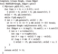
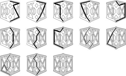
Figure 22.17 Shortest augmenting paths

This sequence illustrates how the shortest-augmenting-path implementation of the Ford–Fulkerson method finds a maximum flow in a sample network. Path lengths increase as the algorithm progresses: The first four paths in the top row are of length 3; the last path in the top row and all of the paths in the second row are of length 4; the first two paths in the bottom row are of length 5; and the process finishes with two paths of length 7 that each have a backward edge.

from the figure, the lengths of the augmenting paths form a nondecreasing sequence. Our analysis of this method, in Property 22.7, proves that this property is characteristic.

Another Ford–Fulkerson implementation suggested by Edmonds and Karp is the following: Augment along the path that increases the flow by the largest amount. The priority value P that is used in Program 22.3 implements this method. This priority makes the algorithm choose edges from the fringe to give the maximum amount of flow that can be pushed through a forward edge or diverted from a backward edge. For brevity, we refer to this method as the maximum-capacity– augmenting-path maxflow algorithm. Program 22.18 illustrates the algorithm on the same flow network as that in Program 22.17.

These are but two examples (ones we can analyze!) of Ford– Fulkerson implementations. At the end of this section, we consider others. Before doing so, we consider the task of analyzing augmenting-path methods in order to learn their properties and, ultimately, to decide which one will have the best performance.

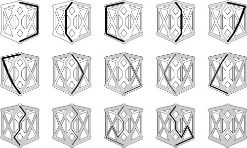
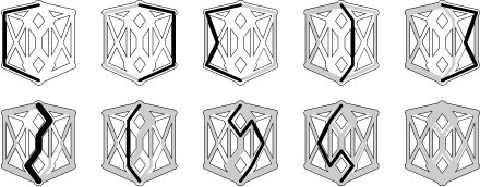
Figure 22.18 Maximum-capacity augmenting paths

This sequence illustrates how the maximum-capacity–augmenting-path implementation of the Ford– Fulkerson method finds a maxflow in a sample network. Path capacities decrease as the algorithm progresses, but their lengths may increase or decrease. The method needs only nine augmenting paths to compute the same maxflow as the one depicted in Program 22.17.

In trying to choose among the family of algorithms represented by Program 22.3, we are in a familiar situation. Should we focus on worst-case performance guarantees, or do those represent a mathematical fiction that may not relate to networks that we encounter in practice? This question is particularly relevant in this context, because the classical worst-case performance bounds that we can establish are much higher than the actual performance results that we see for typical graphs.

Many factors further complicate the situation. For example, the worst-case running time for several versions depends not just on V and E, but also on the values of the edge capacities in the network. Developing a maxflow algorithm with fast guaranteed performance has been a tantalizing problem for several decades, and numerous methods have been proposed. Evaluating all these methods for all the types of networks that are likely to be encountered in practice, with sufficient precision to allow us to choose among them, is not as clear-cut as is the same task for other situations that we have studied, such as typical practical applications of sorting or searching algorithms.

Keeping these difficulties in mind, we now consider the classical results about the worst-case performance of the Ford–Fulkerson method: One general bound and two specific bounds, one for each of the two augmenting-path algorithms that we have examined. These results serve more to give us insight into characteristics of the algorithms than to allow us to predict performance to a sufficient degree of accuracy

Figure 22.19 Two scenarios for the Ford– Fulkerson algorithm

This network illustrates that the number of iterations used by the Ford–Fulkerson algorithm depends on the capacities of the edges in the network and the sequence of paths chosen by the implementation. It consists of four edges of capacity X and one of capacity 1. The scenario depicted at the top shows that an implementation that alternates between using 0-1-2-3 and 0-2-1-3 as augmenting paths (for example, one that prefers long paths) would require X pairs of iterations like the two pairs shown, each pair incrementing the total flow by 2. The scenario depicted at the bottom shows that an implementation that chooses 0-1-3 and then 0-2-3 as augmenting paths (for example, one that prefers short paths) finds the maximum flow in just two iterations.

for meaningful comparison. We discuss empirical comparisons of the methods at the end of the section.

If edge capacities are, say, 32-bit integers, the scenario depicted at the top would be billions of times slower than the scenario depicted the bottom.

Property 22.6 Let M be the maximum edge capacity in the network. The number of augmenting paths needed by any implementation of the Ford–Fulkerson algorithm is at most equal to VM.

Proof: Any cut has at most V edges, of capacity M, for a total capacity of VM. Every augmenting path increases the flow through every cut by at least 1, so the algorithm must terminate after VM passes, since all cuts must be filled to capacity after that many augmentations.

As discussed below, such a bound is of little use in typical situations because M can be a very large number. Worse, it is easy to describe situations where the number of iterations is proportional to the maximum edge capacity. For example, suppose that we use a longest augmenting-path algorithm (perhaps based on the intuition that the longer the path, the more flow we put on the network’s edges). Since we are counting iterations, we ignore, for the moment, the cost of computing such a path. The (classical) example shown in Figure 22.19 shows a network for which the number of iterations of a longest augmenting-path algorithm is equal to the maximum edge capacity. This example tells us that we must undertake a more detailed scrutiny to know whether other specific implementations use substantially fewer iterations than are indicated by Property 22.6.

For sparse networks and networks with small integer capacities, Property 22.6 does give an upper bound on the running time of any Ford–Fulkerson implementation that is useful.

Corollary The time required to find a maxflow is O (V EM), which is O(V²M)for sparse networks.

Proof: Immediate from the basic result that generalized graph search is linear in the size of the graph representation (Property 18.12). As mentioned, we need an extra lg V factor if we are using a priority-queue fringe implementation.

The proof actually establishes that the factor of M can be replaced by the ratio between the largest and smallest nonzero capacities in the network (see Exercise 22.25). When this ratio is low, the bound tells us that any Ford–Fulkerson implementation will find a maxflow in time proportional to the time required to (for example) solve the all-shortest-paths problem, in the worst case. There are many situations where the capacities are indeed low and the factor of M is of no concern. We will see an example in Section 22.4.

When M is large, the V EM worst-case bound is high; but it is pessimistic, as we obtained it by multiplying together worst-case bounds that derive from contrived examples. Actual costs on practical networks are typically much lower.

From a theoretical standpoint, our first goal is to discover, using the rough subjective categorizations of Section 17.8, whether or not the maximum-flow problem for networks with large integer weights is tractable (solvable by a polynomial-time algorithm). The bounds just derived do not resolve this question, because the maximum weight M = 2^m could grow exponentially with V and E. From a practical standpoint, we seek better performance guarantees. To pick a typical practical example, suppose that we use 32-bit integers (m = 32) to represent edge weights. In a graph with hundreds of vertices and thousands of edges, the corollary to Property 22.6 says that we might have to perform hundreds of trillions of operations in an augmenting-path algorithm. If we are dealing with millions of vertices, this point is moot, not only because we will not have weights as large 2^1000000, but also because V³ and V E are so large as to make the bound meaningless. We are interested both in finding a polynomial bound to resolve the tractability question and in finding better bounds that are relevant for situations that we might encounter in practice.

Property 22.6 is general: It applies to any Ford–Fulkerson implementation at all. The generic nature of the algorithm leaves us with a substantial amount of flexibility to consider a number of simple implementations in seeking to improve performance. We expect that specific implementations might be subject to better worst-case bounds. Indeed, that is one of our primary reasons for considering them in the first place! Now, as we have seen, implementing and using a large class of these implementations is trivial: We just substitute different generalized-queue implementations or priority definitions in Program 22.3. Analyzing differences in worst-case behavior is more challenging, as indicated by the classical results that we consider next for the two basic augmenting-path implementations that we have considered.

First, we analyze the shortest-augmenting-path algorithm. This method is not subject to the problem illustrated in Program 22.19. Indeed, we can use it to replace the factor of M in the worst-case running time with V E/ 2, thus establishing that the network-flow problem is tractable. We might even classify it as being easy (solvable in polynomial time on practical cases by a simple, if clever, implementation).

Property 22.7 The number of augmenting paths needed in the shortest-augmenting-path implementation of the Ford–Fulkerson algorithm is at most V E/ 2.

Proof: First, as is apparent from the example in Program 22.17, no augmenting path is shorter than a previous one. To establish this fact, we show by contradiction that a stronger property holds: No augmenting path can decrease the length of the shortest path from the source s to any vertex in the residual network. Suppose that some augmenting path does so, and that v is the first such vertex on the path. There are two cases to consider: Either no vertex on the new shorter path from s to v appears anywhere on the augmenting path or some vertex w on the new shorter path from s to v appears somewhere between v and t on the augmenting path. Both situations contradict the minimality of the augmenting path.

Now, by construction, every augmenting path has at least one critical edge: an edge that is deleted from the residual network because it corresponds either to a forward edge that becomes filled to capacity or a backward edge that is emptied. Suppose that an edge u-v is a critical edge for an augmenting path P of length d. The next augmenting path for which it is a critical edge has to be of length at least d+2, because that path has to go from s to v, then along v-u, then from u to t. The first segment is of length at least 1 greater than the distance from s to u in P, and the final segment is of length at least 1 greater than the distance from v to t in P, so the path is of length at least 2 greater than P.

Since augmenting paths are of length at most V, these facts imply that each edge can be the critical edge on at most V/ 2 augmenting paths, so the total number of augmenting paths is at most EV/ 2.

Corollary The time required to find a maxflow in a sparse network is O (V³).

Proof: The time required to find an augmenting path is O (E), so the total time is O (V E²). The stated bound follows immediately.

The quantity V³ is sufficiently high that it does not provide a guarantee of good performance on huge networks. But that fact should not preclude us from using the algorithm on a huge network, because it is a worst-case performance result that may not be useful for predicting performance in a practical application. For example, as just mentioned, the maximum capacity M (or the maximum ratio between capacities) might be much less than V, so the corollary to Property 22.6 would provide a better bound. Indeed, in the best case, the number of augmenting paths needed by the Ford–Fulkerson method is the smaller of the outdegree of s or the indegree of t, which again might be far smaller than V. Given this range between best- and worst-case performance, comparing augmenting-path algorithms solely on the basis of worst-case bounds is not wise.

Still, other implementations that are nearly as simple as the shortest-augmenting-path method might admit better bounds or be preferred in practice (or both). For example, the maximum-augmenting-path algorithm used far fewer paths to find a maxflow than did the shortest-augmenting-path algorithm in the example illustrated in Figures 22.17 and 22.18. We now turn to the worst-case analysis of that algorithm.

First, just as for Prim’s algorithm and for Dijkstra’s algorithm (see Sections 20.6 and 21.2), we can implement the priority queue such that the algorithm takes time proportional to V² (for dense graphs) or (E + V) log V (for sparse graphs) per iteration in the worst case, although these estimates are pessimistic because the algorithm stops

Figure 22.20 Stack-based augmenting-path search

This illustrates the result of using a stack for the generalized queue in our implementation of the Ford– Fulkerson method, so that the path search operates like DFS. In this case, the method does about as well as BFS, but its somewhat erratic behavior is rather sensitive to the network representation and has not been analyzed.

when it reaches the sink. We also have seen that we can do slightly better with advanced data structures. The more important and more challenging question is how many augmenting paths are needed.

Property 22.8 The number of augmenting paths needed in the maximal-augmenting-path implementation of the Ford–Fulkerson algorithm is at most 2E lg M.

Proof: Given a network, let F be its maxflow value. Let v be the value of the flow at some point during the algorithm as we begin to look for an augmenting path. Applying Property 22.2 to the residual network, we can decompose the flow into at most E directed paths that sum to F − v, so the flow in at least one of the paths is at least (F − v)/E. Now, either we find the maxflow sometime before doing another 2E augmenting paths or the value of the augmenting path after that sequence of 2E paths is less than (F − v)/2E, which is less than one-half of the value of the maximum before that sequence of 2E paths. That is, in the worst case, we need a sequence of 2E paths to

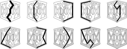
Figure 22.21 Randomized augmenting-path search

This sequence the result of using a randomized queue for the fringe data structure in the augmenting-path search in the Ford–Fulkerson method. In this example, we happen upon the short high-capacity path and therefore need relatively few augmenting paths. While predicting the performance characteristics of this method is a challenging task, it performs well in many situations.

decrease the path value by a factor of 2. The first path value is at most M, which we need to decrease by a factor of 2 at most lg M times, so we have a total of at most lg M sequences of 2E paths.

Corollary The time required to find a maxflow in a sparse network is O (V² lg M lg V ).

Proof: Immediate from the use of a heap-based priority-queue implementation, as for Properties 20.7 and 21.5.

For values of M and V that are typically encountered in practice, this bound is significantly lower than the O (V³) bound of the corollary to Property 22.7. In many practical situations, the maximum-augmenting-path algorithm uses significantly fewer iterations than does the shortest-augmenting-path algorithm, at the cost of a slightly higher bound on the work to find each path.

There are many other variations to consider, as reflected by the extensive literature on maxflow algorithms. Algorithms with better worst-case bounds continue to be discovered, and no nontrivial lower bound has been proved—that is, the possibility of a simple linear-time algorithm remains. Although they are important from a theoretical standpoint, many of the algorithms are primarily designed to lower the worst-case bounds for dense graphs, so they do not offer substantially better performance than the maximum-augmenting-path algorithm for the kinds of sparse networks that we encounter in practice. Still, there remain many options to explore in pursuit of better practical maxflow algorithms. We briefly consider two more augmenting-path algorithms next; in Section 22.3, we consider another family of algorithms.

One easy augmenting-path algorithm is to use the value of a decreasing counter for P or a stack implementation for the generalized queue in Program 22.3, making the search for augmenting paths like depth-first search. Figure 22.20 shows the flow computed for our small example by this algorithm. The intuition is that the method is fast, is easy to implement, and appears to put flow throughout the network. As we will see, its performance varies remarkably, from extremely poor on some networks to reasonable on others.

Another alternative is to use a randomized-queue implementation for the generalized queue so that the search for augmenting paths is a randomized search. Program 22.21 shows the flow computed for our small example by this algorithm. This method is also fast and easy to implement; in addition, as we noted in Section 18.8, it may embody good features of both breadth-first and depth-first search. Randomization is a powerful tool in algorithm design, and this problem represents a reasonable situation in which to consider using it.

We conclude this section by looking more closely at the methods that we have examined in order to see the difficulty of comparing them or attempting to predict performance for practical applications.

As a start in understanding the quantitative differences that we might expect, we use two flow-network models that are based on the Euclidean graph model that we have been using to compare other graph algorithms. Both models use a graph drawn from V points in the plane with random coordinates between 0 and 1 with edges connecting any two points within a fixed distance of each other. They differ in the assignment of capacities to the edges.

The first model simply assigns the same constant value to each capacity. As discussed in Section 22.4, this type of network-flow problem is known to be easier than the general problem. For our Euclidean graphs, flows are limited by the outdegree of the source and the indegree of the sink, so the algorithms each need only a few augmenting paths. But the paths differ substantially for the various algorithms, as we soon see.

The second model assigns random weights from some fixed range of values to the capacities. This model generates the type of networks that people typically envision when thinking about the problem, and

Figure 22.22 Random flow networks

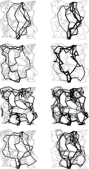
This figure depicts maxflow computations on our random Euclidean graph, with two different capacity models. On the left, all edges are assigned unit capacities; on the right, edges are assigned random capacities. The source is near the middle at the top and the sink near the middle at the bottom. Illustrated top to bottom are the flows computed by the shortest-path, maximum-capacity, stack-based, and randomized algorithms, respectively. Since the vertices are not of high degree and the capacities are small integers, there are many different flows that achieve the maximum for these examples.

The indegree of the sink is 6, so all the algorithms find the flow in the unit-capacity model on the left with six augmenting paths.

The methods find augmenting paths that differ dramatically in character for the random-weight model on the right. In particular, the stack-based method finds long paths of low weight and even produces a flow with a disconnected cycle.

Table 22.1 Empirical study of augmenting-path algorithms

This table shows performance parameters for various augmenting-path network-flow algorithms for our sample Euclidean neighbor network (with random capacities with maxflow value 286) and with unit capacities (with maxflow value 6). The maximum-capacity algorithm outperforms the others for both types of networks. The random search algorithm finds augmenting paths that are not much longer than the shortest, and examines fewer nodes. The stack-based algorithm peforms very well for random weights but, though it has very long paths, is competetive for unit weights.

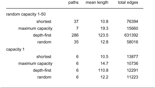
the performance of the various algorithms on such networks is certainly instructive.

Both of these models are illustrated in Program 22.22, along with the flows that are computed by the four methods on the two networks. Perhaps the most noticeable characteristic of these examples is that the flows themselves are different in character. All have the same value, but the networks have many maxflows, and the different algorithms make different choices when computing them. This situation is typical in practice. We might try to impose other conditions on the flows that we want to compute, but such changes to the problem can make it more difficult. The mincost-flow problem that we consider in Sections 22.5 through 22.7 is one way to formalize such situations.

Table 22.1 gives more detailed quantitative results for use of the four methods to compute the flows in Program 22.22. An augmenting-path

Figure 22.23 Maximum-capacity augmenting paths (larger example)

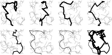
This figure depicts the augmenting paths computed by the maximum-capacity algorithm for the Euclidean network with random weights that is shown in Program 22.22, along with the edges in the graph-search spanning tree (in gray). The resulting flow is shown at the bottom right.

algorithm’s performance depends not just on the number of augmenting paths but also on the lengths of such paths and on the cost of finding them. In particular, the running time is proportional to the number of edges examined in the inner loop of Program 22.3. As usual, this number might vary widely, even for a given graph, depending on properties of the representation; but we can still characterize different algorithms. For example, Figures 22.23 and 22.24 show the search trees for the maximum-capacity and shortest-path algorithms, respectively. These examples help support the general conclusion that the shortest-path method expends more effort to find augmenting paths with less flow than the maximum-capacity algorithm, thus helping to explain why the latter is preferred.

Perhaps the most important lesson that we can learn from studying particular networks in detail in this way is that the gap between the upper bounds of Properties 22.6 through 22.8 and the actual number of augmenting paths that the algorithms need for a given application might be enormous. For example, the flow network illustrated in Program 22.23 has 177 vertices and 2000 edges of capacity less than 100, so the value of the quantity 2E lg M in Property 22.8 is more than 25,000; but the maximum-capacity algorithm finds the maxflow with only seven augmenting paths. Similarly, the value of the quantity V E/2 in Property 22.7 for this network is 177,000, but the shortest-path algorithm needs only 37 paths.

As we have already indicated, the relatively low node degree and the locality of the connections partially explain these differences between theoretical and actual performance in this case. We can prove more accurate performance bounds that account for such details; but such disparities are the rule, not the exception, in flow-network models and in practical networks. On the one hand, we might take these results to indicate that these networks are not sufficiently general to represent the networks that we encounter in practice; on the other hand, perhaps the worst-case analysis is more removed from practice than these kinds of networks.

Large gaps like this certainly provide strong motivation for researchers seeking to lower the worst-case bounds. There are many other possible implementations of augmenting-path algorithms to consider that might lead to better worst-case performance or better practical performance than the methods that we have considered (see Exercises 22.56 through 22.60). Numerous methods that are more sophisticated and have been shown to have improved worst-case performance can be found in the research literature (see reference section).

Another important complication follows when we consider the numerous other problems that reduce to the maxflow problem. When such reductions apply, the flow networks that result may have some special structure that some particular algorithm may be able to exploit for improved performance. For example, in Section 22.8 we will examine a reduction that gives flow networks with unit capacities on all edges.

Even when we restrict attention just to augmenting-path algorithms, we see that the study of maxflow algorithms is both an art and a science. The art lies in picking the strategy that is most effective for a given practical situation; the science lies in understanding the essential nature of the problem. Are there new data structures and algorithms that can solve the maxflow problem in linear time, or can we prove that none exist? In Section 22.3, we see that no augmenting-path algorithm can have linear worst-case performance, and we examine a different generic family of algorithms that might.

Figure 22.24 Shortest augmenting paths (larger example)

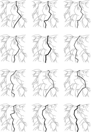
This figure depicts the augmenting paths computed by the shortest-paths algorithm for the Euclidean network with random weights that is shown in Program 22.22, along with the edges in the graph-search spanning tree (in gray). In this case, this algorithm is much slower than the maximum-capacity algorithm depicted in Program 22.23 both because it requires a large number of augmenting paths (the paths shown are just the first 12 out of a total of 37) and because the spanning trees are larger (usually containing nearly all of the vertices).

Exercises

22.19 Show, in the style of Program 22.13, as many different sequences of augmenting paths as you can find for the flow network shown in Program 22.10.

22.20 Show, in the style of Program 22.15, all the cuts for the flow network shown in Program 22.10, their cut sets, and their capacities.

• 22.21 Find a minimum cut in the flow network shown in Program 22.11.

• 22.22 Suppose that capacities are in equilibrium in a flow network (for every internal node, the total capacity of incoming edges is equal to the total capacity of outgoing edges). Does the Ford–Fulkerson algorithm ever use a backward edge? Prove that it does or give a counterexample.

22.23 Give a maxflow for the flow network shown in Program 22.5 with at least one flow that is not an integer.

• 22.24 Develop an implementation of the Ford–Fulkerson algorithm that uses a generalized queue instead of a priority queue (see Section 18.8).

• 22.25 Prove that the number of augmenting paths needed by any implementation of the Ford–Fulkerson algorithm is no more than V times the smallest integer larger than the ratio of the largest edge capacity to the smallest edge capacity.

22.26 Prove a linear-time lower bound for the maxflow problem: Show that, for any values of V and E, any maxflow algorithm might have to examine every edge in some network with V vertices and E edges.

• 22.27 Give a network like Program 22.19 for which the shortest-augmenting-path algorithm has the worst-case behavior that is illustrated.

22.28 Give an adjacency-lists representation of the network in Program 22.19 for which our implementation of the stack-based search (Program 22.3, using a stack for the generalized queue) has the worst-case behavior that is illustrated.

22.29 Show, in the style of Program 22.16, the flow and residual networks after each augmenting path when we use the shortest-augmenting-path algorithm to find a maxflow in the flow network shown in Program 22.10. Also include the graph-search trees for each augmenting path. When more than one path is possible, show the one that is chosen by the implementations given in this section.

22.30 Do Exercise 22.29 for the maximum-capacity–augmenting-path algorithm.

22.31 Do Exercise 22.29 for the stack-based–augmenting-path algorithm.

• 22.32 Exhibit a family of networks for which the maximum-augmenting-path algorithm needs 2E lg M augmenting paths.

• 22.33 Can you arrange the edges such that our implementations take time proportional to E to find each path in your example in Exercise 22.32? If necessary, modify your example to achieve this goal. Describe the adjacency-lists representation that is constructed for your example. Explain how the worst case is achieved.

22.34 Run empirical studies to determine the number of augmenting paths and the ratio of the running time to V for each of the four algorithms described in this section, for various networks (see Exercises 22.7–12).

22.35 Develop and test an implementation of the augmenting-path method that uses the source–sink shortest-path heuristic for Euclidean networks of Section 21.5.

22.36 Develop and test an implementation of the augmenting-path method that is based on alternately growing search trees rooted at the source and at the sink (see Exercises 21.35 and 21.75).

• 22.37 The implementation of Program 22.3 stops the graph search when it finds the first augmenting path from source to sink, augments, then starts the search all over again. Alternatively, it could go on with the search and find another path, continuing until all vertices have been marked. Develop and test this second approach.

22.38 Develop and test implementations of the augmenting-path method that use paths that are not simple.

• 22.39 Give a sequence of simple augmenting paths that produces a flow with a cycle in the network depicted in Program 22.11.

• 22.40 Give an example showing that not all maxflows can be the result of starting with an empty network and augmenting along a sequence of simple paths from source to sink.

22.41 [Gabow] Develop a maxflow implementation that uses m = lg M phases, where the i th phase solves the maxflow problem using the leading i bits of the capacities. Start with zero flow everywhere; then, after the first phase, initialize the flow by doubling the flow found during the previous phase. Run empirical studies for various networks (see Exercises 22.7–12) to compare this implementation to the basic methods.

• 22.42 Prove that the running time of the algorithm described in Exercise 22.41 is O (V E lg M ).

22.43 Experiment with hybrid methods that use one augmenting-path method at the beginning, then switch to a different augmenting path to finish up (part of your task is to decide what are appropriate criteria for when to switch). Run empirical studies for various networks (see Exercises 22.7–12) to compare these to the basic methods, studying methods that perform better than others in more detail.

22.44 Experiment with hybrid methods that alternate between two or more different augmenting-path methods. Run empirical studies for various networks (see Exercises 22.7–12) to compare these to the basic methods, studying variations that perform better than others in more detail.

• 22.45 Experiment with hybrid methods that choose randomly among two or more different augmenting-path methods. Run empirical studies for various networks (see Exercises 22.7–12) to compare these to the basic methods, studying variations that perform better than others in more detail.

• 22.46 Write a flow-network client function that, given an integer c, finds an edge for which increasing the capacity of that edge by c increases the maxflow by the maximum amount. Your function may assume that the client has already computed a maximum flow with MAXFLOW.

•• 22.47 Suppose that you are given a mincut for a network. Does this information make it easier to compute a maxflow? Develop an algorithm that uses a given mincut to speed up substantially the search for maximum-capacity augmenting paths.

• 22.48 Write a client program that does dynamic graphical animations of augmenting-path algorithms. Your program should produce images like Program 22.17 and the other figures in this section (see Exercises 17.55–59). Test your implementation for the Euclidean networks among Exercises 22.7–12.

22.3 Preflow-Push Maxflow Algorithms

In this section, we consider another approach to solving the maxflow problem. Using a generic method known as the preflow-push method, we incrementally move flow along the outgoing edges of vertices that have more inflow than outflow. The preflow-push approach was developed by A. Goldberg and R. E. Tarjan in 1986 on the basis of various earlier algorithms. It is widely used because of its simplicity, flexibility, and efficiency.

As defined in Section 22.1, a flow must satisfy the equilibrium conditions that the outflow from the source is equal to the inflow to the sink and that inflow is equal to the outflow at each of the internal nodes. We refer to such a flow as a feasible flow. An augmenting-path algorithm always maintains a feasible flow: It increases the flow along augmenting paths until a maxflow is achieved. By contrast, the preflow-push algorithms that we consider in this section maintain maxflows that are not feasible because some vertices have more inflow than outflow: They push flow through such vertices until a feasible flow is achieved (no such vertices remain).

Definition 22.5 In a flow network, a preflow is a set of positive edge flows satisfying the conditions that the flow on each edge is no greater than that edge’s capacity and that inflow is no smaller than outflow

Figure 22.25 Preflow-push example

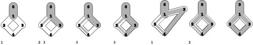
In the preflow-push algorithm, we maintain a list of the active nodes that have more incoming than outgoing flow (shown below each network). One version of the algorithm is a loop that chooses an active node from the list and pushes flow along outgoing edges until it is no longer active, perhaps creating other active nodes in the process. In this example, we push flow along 0-1, which makes 1 active. Next, we push flow along 1-2 and 1-3, which makes 1 inactive but 2 and 3 both active. Then, we push flow along 2-4, which makes 2 inactive. But 3-4 does not have sufficient capacity for us to push flow along it to make 3 inactive, so we also push flow back along 3-1 to do so, which makes 1 active. Then we can push the flow along 1-2 and then 2-4, which makes all nodes inactive and leaves a maxflow.

for every internal vertex. An active vertex is an internal vertex whose inflow is larger than its outflow (by convention, the source and sink are never active).

We refer to the difference between an active vertex’s inflow and outflow as that vertex’s excess. To change the set of active vertices, we choose one and push its excess along an outgoing edge, or, if there is insufficient capacity to do so, push the excess back along an incoming edge. If the push equalizes the vertex’s inflow and outflow, the vertex becomes inactive; the flow pushed to another vertex may activate that vertex. The preflow-push method provides a systematic way to push excess out of active vertices repeatedly so that the process terminates in a maxflow, with no active vertices. We keep active vertices on a generalized queue. As for the augmenting-path method, this decision gives a generic algorithm that encompasses a whole family of more specific algorithms.

Figure 22.25 is a small example that illustrates the basic operations used in preflow-push algorithms, in terms of the metaphor that we have been using, where we imagine that flow can go only down the page. Either we push excess flow out of an active vertex down an outgoing edge or we imagine that the vertex temporarily moves up so we can push excess flow back down an incoming edge.

Figure 22.26 is an example that illustrates why the preflow-push approach might be preferred to the augmenting-paths approach. In this network, any augmenting-path method successively puts a tiny amount of flow through a long path over and over again, slowly filling up the edges on the path until finally the maxflow is reached. By contrast, the preflow-push method fills up the edges on the long path as it traverses that path for the first time, then distributes that flow directly to the sink without traversing the long path again.

As we did in augmenting-path algorithms, we use the residual network (see Definition 22.4) to keep track of the edges that we might push flow through. Every edge in the residual network represents a potential place to push flow. If a residual-network edge is in the same direction as the corresponding edge in the flow network, we increase the flow; if it is in the opposite direction, we decrease the flow. If the increase fills the edge or the decrease empties the edge, the corresponding edge disappears from the residual network. For preflow-push algorithms, we use an additional mechanism to help decide which of the edges in the residual network can help us to eliminate active vertices.

Definition 22.6 A height function for a given flow in a flow network is a set of nonnegative vertex weights h(0)…h(V− 1)such that h (t)= 0 for the sink t and h(u)≤h(v)+1for every edge u-v in the residual network for the flow. An eligible edge is an edge u-v in the residual network with h(u)=h(v)+1.

Figure 22.26 Bad case for the Ford–Fulkerson algorithm

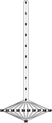
This network represents a family of networks with V vertices for which any augmenting-path algorithm requires V/ 2 paths of length V/2 (since every augmenting path has to include the long vertical path), for a total running time proportional to V². Preflow-push algorithms find maxflows in such networks in linear time.

A trivial height function, for which there are no eligible edges, is h(0)=h(1) =…=h(V − 1) = 0. If we set h(s) = 1, then any edge that emanates from the source and has flow corresponds to an eligible edge in the residual network.

We define a more interesting height function by assigning to each vertex the latter’s shortest-path distance to the sink (its distance to the root in any BFS tree for the reverse of the network rooted at t, as illustrated in Program 22.27). This height function is valid because h(t) = 0, and, for any pair of vertices u and v connected by an edge u-v, any shortest path to t starting with u-v is of length h (v) + 1; so the shortest-path length from u to t, or h (u), must be less than or equal to that value. This function plays a special role because it puts each vertex at the maximum possible height. Working backward, we see that t has to be at height 0; the only vertices that could be at height 1 are those with an edge directed to t in the residual network; the only vertices that could be at height 2 are those that have edges directed to vertices that could be at height 1, and so forth.

Property 22.9 For any flow and associated height function, a vertex’s height is no larger than the length of the shortest path from that vertex to the sink in the residual network.

Proof: For any given vertex u, let d be the shortest-path length from u to t, and let u =u₁, u₂,…, u_d =t be a shortest path. Then

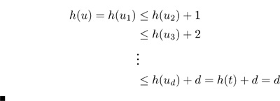
Figure 22.27 Initial height function

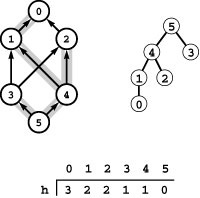
The tree at the right is a BFS tree rooted at 5 for the reverse of our sample network (left). The vertex-indexed array h gives the distance from each vertex to the root and is a valid height function: For every edge u-v in the network, h[u] is less than or equal to h[v]+1.

The intuition behind height functions is the following: When an active node’s height is less than the height of the source, it is possible that there is some way to push flow from that node down to the sink; when an active node’s height exceeds the height of the source, we know that that node’s excess needs to be pushed back to the source. To establish this latter fact, we reorient our view of Property 22.9, where we thought about the length of the shortest path to the sink as an upper bound on the height; instead, we think of the height as a lower bound on the shortest-path length:

Corollary If a vertex’s height is greater than V, then there is no path from that vertex to the sink in the residual network.

Proof: If there is a path from the vertex to the sink, the implication of Property 22.9 would be that the path’s length is greater than V, but that cannot be true because the network has only V vertices.

Now that we understand these basic mechanisms, the generic preflow-push algorithm is simple to describe. We start with any height function and assign zero flow to all edges except those connected to the source, which we fill to capacity. Then, we repeat the following step until no active vertices remain:

We do not specify what the initial height function is, how to choose the active vertex, how to choose the eligible edge, or how much flow to push. We refer to this generic method as the edge-based preflow-push algorithm.

The algorithm depends on the height function to identify eligible edges. We also use the height function both to prove that the algorithm computes a maxflow and to analyze performance. Therefore, it is critical to ensure that the height function remains valid throughout the execution of the algorithm.

Property 22.10 The edge-based–preflow-push algorithm preserves the validity of the height function.

Proof: We increment h(u) only if there are no edges u-v with h(u)=h(v)+1. Thatis, h(u)< h(v)+1 for all edges u-v before incrementing h(u), so h(u)h(v) + 1 afterward. For any incoming edges w-u, incrementing h(u) certainly preserves the inequality h(w)h(u)+1. Incrementing h(u) does not affect inequalities corresponding to any other edge, and we never increment h(t) (or h(s)). Together, these observations imply the stated result.

All the excess flow emanates from the source. Informally, the generic preflow-push algorithm tries to push the excess flow to the sink; if it cannot do so, it eventually pushes the excess flow back to the source. It behaves in this manner because nodes with excess always stay connected to the source in the residual network.

Property 22.11 While the preflow-push algorithm is in execution on a flow network, there exists a (directed) path in that flow network’s residual network from each active vertex to the source, and there are no (directed) paths from source to sink in the residual network.

Proof: By induction. Initially, the only flow is in the edges leaving the source, which are filled to capacity, so the destination vertices of those edges are the only active vertices. Since the edges are filled to capacity, there is an edge in the residual network from each of those vertices to the source and there are no edges in the residual network leaving the source. Thus, the stated property holds for the initial flow.

The source is reachable from every active vertex because the only way to add to the set of active vertices is to push flow from an active vertex down an eligible edge. This operation leaves an edge in the residual network from the receiving vertex back to the active vertex, from which the source is reachable, by the inductive hypothesis.

Initially, no other nodes are reachable from the source in the residual network. The first time that another node u becomes reachable from the source is when flow is pushed back along u-s (thus causing s-u to be added to the residual network). But this can happen only when h(u) is greater than h(s), which can happen only after h(u) has been incremented, because there are no edges in the residual network to vertices with lower height. The same argument shows that all nodes reachable from the source have greater height. But the sink’s height is always 0, so it cannot be reachable from the source.

Corollary During the preflow-push algorithm, vertex heights are always less than 2V.

Proof: We need to consider only active vertices, since the height of each inactive vertex is either the same as or 1 greater than it was the last time that the vertex was active. By the same argument as in the proof of Property 22.9, the path from a given active vertex to the source implies that that vertex’s height is at most V −2 greater than the height of the source (t cannot be on the path). The height of the source never changes, and it is initially no greater than V. Thus, active vertices are of height at most 2V − 2, and no vertex has height 2V or greater.

The generic preflow-push algorithm is simple to state and implement. Less clear, perhaps, is why it computes a maxflow. The height function is the key to establishing that it does so.

Property 22.12 The preflow-push algorithm computes a maxflow.

Proof: First, we have to show that the algorithm terminates. There must come a point where there are no active vertices. Once we push all the excess flow out of a vertex, that vertex cannot become active again until some of that flow is pushed back; and that pushback can happen only if the height of the vertex is increased. If we have a sequence of active vertices of unbounded length, some vertex has to appear an unbounded number of times; and it can do so only if its height grows without bound, contradicting the corollary to Property 22.9.

When there are no active vertices, the flow is feasible. Since, by Property 22.11, there is also no path from source to sink in the residual network, the flow is a maxflow, by the same argument as that in the proof of Property 22.5.

It is possible to refine the proof that the algorithm terminates to give an O(V²E) bound on its worst-case running time. We leave the details to exercises (see Exercises 22.66 through 22.67), in favor of the simpler proof in Property 22.13, which applies to a less general version of the algorithm. Specifically, the implementations that we consider are based on the following more specialized instructions for the iteration:

That is, once we have chosen a vertex, we push out of it as much flow as possible. If we get to the point that the vertex still has excess flow but no eligible edges remain, we increment the vertex’s height. We refer to this generic method as the vertex-based preflow-push algorithm. It is a special case of the edge-based generic algorithm, where we keep choosing the same active vertex until it becomes inactive or we have used up all the eligible edges leaving it. The correctness proof in Property 22.12 applies to any implementation of the edge-based generic algorithm, so it immediately implies that the vertex-based algorithm computes a maxflow.

Program 22.5 is an implementation of the vertex-based generic algorithm that uses a generalized queue for the active vertices. It is a direct implementation of the method just described and represents a family of algorithms that differ only in their initial height function (see, for example, Exercise 22.52) and in their generalized-queue ADT implementation. This implementation assumes that the generalized queue disallows duplicate vertices; alternatively, we could add code to Program 22.5 to avoid enqueueing duplicates (see Exercises 22.61 and 22.62).

Perhaps the simplest data structure to use for active vertices is a FIFO queue. Figure 22.28 shows the operation of the algorithm on a sample network. As illustrated in the figure, it is convenient to break up the sequence of active vertices chosen into a sequence of phases, where a phase is defined to be the contents of the queue after all the vertices that were on the queue in the previous phase have been processed. Doing so helps us to bound the total running time of the algorithm.

Property 22.13 The worst-case running time of the FIFO queue implementation of the preflow-push algorithm is proportional to V²E.

Proof: We bound the number of phases using a potential function. This argument is a simple example of a powerful technique in the

Figure 22.28 Residual networks (FIFO preflow-push)

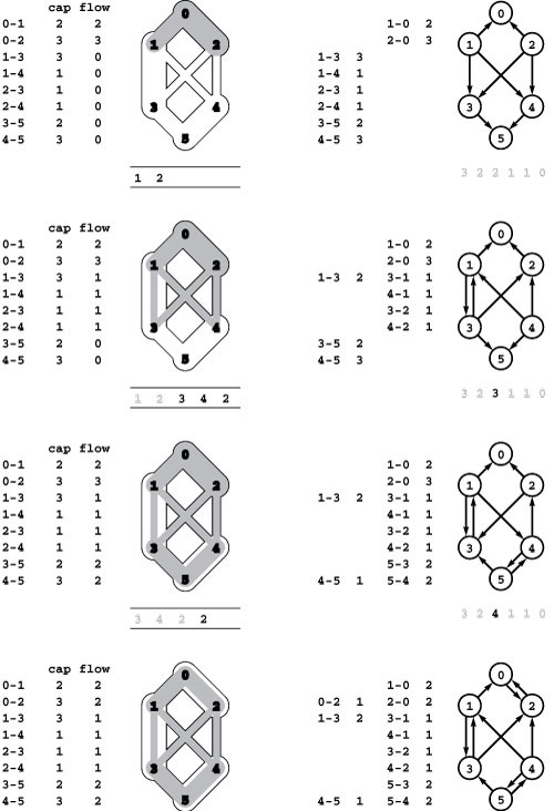
This figure shows the flow networks (left) and the residual networks (right) for each phase of the FIFO preflow-push algorithm operating on our sample network. Queue contents are shown below the flow networks and distance labels below the residual networks. In the initial phase, we push flow through 0-1 and 0-2, thus making 1 and 2 active. In the second phase, we push flow from these two vertices to 3 and 4, which makes them active and 1 inactive (2 remains active and its distance label is incremented). In the third phase, we push flow through 3 and 4 to 5, which makes them inactive (2 still remains active and its distance label is again incremented). In the fourth phase, 2 is the only active node, and the edge 2-0 is admissible because of the distance-label increments, and one unit of flow is pushed back along 2-0 to complete the computation.

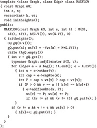
analysis of algorithms and data structures that we examine in more detail in Part 8.

Define the quantity ϕ to be 0 if there are no active vertices and to be the maximum height of the active vertices otherwise, then consider the effect of each phase on the value of ϕ. Let h₀(s) be the initial height of the source. At the beginning, ϕ =h₀(s); at the end, ϕ =0.

First, we note that the number of phases where the height of some vertex increases is no more than 2V²−h₀(s), since each of the V vertex heights can be increased to a value of at most 2V, by the corollary to Property 22.11. Since ϕ can increase only if the height of some vertex increases, the number of phases where ϕ increases is no more than 2V²− h₀(s).

If, however, no vertex’s height is incremented during a phase, then ϕ must decrease by at least 1, since the effect of the phase was to push all excess flow from each active vertex to vertices that have smaller height.

Together, these facts imply that the number of phases must be less than 4V²: The value of ϕ is h₀(s) at the beginning and can be incremented at most 2V²−h₀(s) times and therefore can be decremented at most 2V² times. The worst case for each phase is that all vertices are on the queue and all of their edges are examined, leading to the stated bound on the total running time.

This bound is tight. Program 22.29 illustrates a family of flow networks for which the number of phases used by the preflow-push algorithm is proportional to V².

Because our implementations maintain an implicit representation of the residual network, they examine edges leaving a vertex even when those edges are not in the residual network (to test whether or not they are there). It is possible to show that we can reduce the bound in Property 22.13 from V²E to V³ for an implementation that eliminates this cost by maintaining an explicit representation of the residual network. Although the theoretical bound is the lowest that we have seen for the maxflow problem, this change may not be worth the trouble, particularly for the sparse graphs that we see in practice (see Exercises 22.63 through 22.65).

Again, these worst-case bounds tend to be pessimistic and thus not necessarily useful for predicting performance on real networks (though the gap is not as excessive as we found for augmenting-path

Figure 22.29 FIFO preflow-push worst case

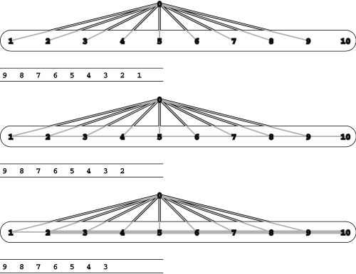
This network represents a family of networks with V vertices such that the total running time of the preflow-push algorithm is proportional to V². It consists of unit-capacity edges emanating from the source (vertex 0) and horizontal edges of capacity v− 2 running from left to right towards the sink (vertex 10). In the initial phase of the preflow-push algorithm (top), we push one unit of flow out each edge from the source, making all the vertices active except the source and the sink. In a standard adjacency-lists representation, they appear on the FIFO queue of active vertices in reverse order, as shown below the network. In the second phase (center), we push one unit of flow from 9 to 10, making 9 inactive (temporarily); then we push one unit of flow from 8 to 9, making 8 inactive (temporarily) and making 9 active; then we push one unit of flow from 7 to 8, making 7 inactive (temporarily) and making 8 active; and so forth. Only 1 is left inactive. In the third phase (bottom), we go through a similar process to make 2 inactive, and the same process continues for V − 2 phases.

algorithms). For example, the FIFO algorithm finds the flow in the network illustrated in Program 22.30 in 15 phases, whereas the bound in the proof of Property 22.13 says only that it must do so in fewer than 182.

To improve performance, we might try using a stack, a randomized queue, or any other generalized queue in Program 22.5. One approach that has proved to do well in practice is to implement the generalized queue such that GQget returns the highest active vertex. We refer to this method as the highest-vertex–preflow-push maxflow algorithm. We can implement this strategy with a priority queue, although it is also possible to take advantage of the particular properties of heights to implement the generalized-queue operations in constant time. A worst-case time bound of V² (which is V^5/2 for sparse graphs) has been proved for this algorithm (see reference section); as usual, this bound is pessimistic. Many other preflow-push variants have been proposed, several of which reduce the worst-case time bound to be close to V E (see reference section).

Table 22.2 shows performance results for preflow-push algorithms corresponding to those for augmenting-path algorithms in Table

Figure 22.30 Preflow-push algorithm (FIFO)

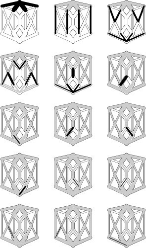
This sequence illustrates how the FIFO implementation of the preflow-push method finds a maximum flow in a sample network. It proceeds in phases: First it pushes as much flow as it can from the source along the edges leaving the source (top left). Then, it pushes flow from each of those nodes, continuing until all nodes are in equilibrium.

Table 22.2 Empirical study of preflow-push algorithms

This table shows performance parameters (number of vertices expanded and number of adjacency-list nodes touched) for various preflow-push network-flow algorithms for our sample Euclidean neighbor network (with random capacities with maxflow value 286) and with unit capacities (with maxflow value 6). Differences among the methods are minimal for both types of networks. For random capacities, the number of edges examined is about the same as for the random augmenting-path algorithm (see Table 22.1). For unit capacities, the augmenting-path algorithms examine substantially fewer edges for these networks.

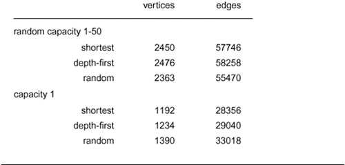
22.1, for the two network models discussed in Section 22.2. These experiments show much less performance variation for the various preflow-push methods than we observed for augmenting-path methods.

There are many options to explore in developing preflow-push implementations. We have already discussed three major choices:

• Edge-based versus vertex-based generic algorithm

• Generalized queue implementation

• Initial assignment of heights

There are several other possibilities to consider and many options to try for each, leading to a multitude of different algorithms to study (see, for example, Exercises 22.56 through 22.60). The dependence of an algorithm’s performance on characteristics of the input network further multiplies the possibilities.

The two generic algorithms that we have discussed (augmenting-path and preflow-push) are among the most important from an extensive research literature on maxflow algorithms. The quest for better maxflow algorithms is still a potentially fruitful area for further research. Researchers are motivated to develop and study new algorithms and implementations by the reality of faster algorithms for practical problems and by the possibility that a simple linear algorithm exists for the maxflow problem. Until one is discovered, we can work confidently with the algorithms and implementations that we have discussed; numerous studies have shown them to be effective for a broad range of practical maxflow problems.

Exercises

• 22.49 Describe the operation of the preflow-push algorithm in a network whose capacities are in equilibrium.

22.50 Use the concepts described in this section (height functions, eligible edges, and pushing of flow through edges) to describe augmenting-path maxflow algorithms.

22.51 Show, in the style of Program 22.28, the flow and residual networks after each phase when you use the FIFO preflow-push algorithm to find a maxflow in the flow network shown in Program 22.10.

• 22.52 Implement the initheights() function for Program 22.5, using breadth-first search from the sink.

22.53 Do Exercise 22.51 for the highest-vertex–preflow-push algorithm.

• 22.54 Modify Program 22.5 to implement the highest-vertex–preflow-push algorithm, by implementing the generalized queue as a priority queue. Run empirical tests so that you can add a line to Table 22.2 for this variant of the algorithm.

22.55 Plot the number of active vertices and the number of vertices and edges in the residual network as the FIFO preflow-push algorithm proceeds, for specific instances of various networks (see Exercises 22.7–12).

• 22.56 Implement the generic edge-based–preflow-push algorithm, using a generalized queue of eligible edges. Run empirical studies for various networks (see Exercises 22.7–12) to compare these to the basic methods, studying generalized-queue implementations that perform better than others in more detail.

22.57 Modify Program 22.5 to recalculate the vertex heights periodically to be shortest-path lengths to the sink in the residual network.

• 22.58 Evaluate the idea of pushing excess flow out of vertices by spreading it evenly among the outgoing edges, rather than perhaps filling some and leaving others empty.

22.59 Run empirical tests to determine whether the shortest-paths computation for the initial height function is justified in Program 22.5 by comparing its performance as given for various networks (see Exercises 22.7–12) with its performance when the vertex heights are just initialized to zero.

• 22.60 Experiment with hybrid methods involving combinations of the ideas above. Run empirical studies for various networks (see Exercises 22.7–12) to compare these to the basic methods, studying variations that perform better than others in more detail.

22.61 Modify the implementation of Program 22.5 such that it explicitly disallows duplicate vertices on the generalized queue. Run empirical tests for various networks (see Exercises 22.7–12) to determine the effect of your modification on actual running times.

22.62 What effect does allowing duplicate vertices on the generalized queue have on the worst-case running-time bound of Property 22.13?

22.63 Modify the implementation of Program 22.5 to maintain an explicit representation of the residual network.

• 22.64 Sharpen the bound in Property 22.13 to O (V³) for the implementation of Exercise 22.63. Hint: Prove separate bounds on the number of pushes that correspond to deletion of edges in the residual network and on the number of pushes that do not result in full or empty edges.

22.65 Run empirical studies for various networks (see Exercises 22.7–12) to determine the effect of using an explicit representation of the residual network (see Exercise 22.63) on actual running times.

22.66 For the edge-based generic preflow-push algorithm, prove that the number of pushes that correspond to deleting an edge in the residual network is less than 2V E. Assume that the implementation keeps an explicit representation of the residual network.

• 22.67 For the edge-based generic preflow-push algorithm, prove that the number of pushes that do not correspond to deleting an edge in the residual network is less than 4V²(V + E ). Hint: Use the sum of the heights of the active vertices as a potential function.

• 22.68 Run empirical studies to determine the actual number of edges examined and the ratio of the running time to V for several versions of the preflow-push algorithm for various networks (see Exercises 22.7–12). Consider various algorithms described in the text and in the previous exercises, and concentrate on those that perform the best on huge sparse networks. Compare your results with your result from Exercise 22.34.

• 22.69 Write a client program that does dynamic graphical animations of preflow-push algorithms. Your program should produce images like Program 22.30 and the other figures in this section (see Exercise 22.48). Test your implementation for the Euclidean networks among Exercises 22.7–12.

Figure 22.31 Reduction from multiple sources and sinks

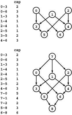
The network at the top has three sources (0, 1, and 2) and two sinks (5 and 6). To find a flow that maximizes the total flow out of the sources and into the sinks, we find a maxflow in the st-network illustrated at the bottom. This network is a copy of the original network, with the addition of a new source 7 and a new sink 8. There is an edge from 7 to each original-network source with capacity equal to the sum of the capacities of that source’s outgoing edges, and an edge from each original-network sink to 8 with capacity equal to the sum of the capacities of that sink’s incoming edges.

22.4 Maxflow Reductions

In this section, we consider a number of reductions to the maxflow problem in order to demonstrate that the maxflow algorithms of Sections 22.2 and 22.3 are important in a broad context. We can remove various restrictions on the network and solve other flow problems; we can solve other network- and graph-processing problems; and we can solve problems that are not network problems at all. This section is devoted to examples of such uses—to establish maxflow as a general problem-solving model.

We also consider relationships between the maxflow problem and problems that are more difficult so as to set the context for considering those problems later on. In particular, we note that the maxflow problem is a special case of the mincost-flow problem that is the subject of Sections 22.5 and 22.6, and we describe how to formulate maxflow problems as LP problems, which we will address in Part 8. Mincost flow and LP represent problem-solving models that are more general than the maxflow model. Although we normally can solve maxflow problems more easily with the specialized algorithms of Sections 22.2 and 22.3 than with algorithms that solve these more general problems, it is important to be cognizant of the relationships among problem-solving models as we progress to more powerful ones.

We use the term standard maxflow problem to refer to the version of the problem that we have been considering (maxflow in edge-capacitated st-networks). This usage is solely for easy reference in this section. Indeed, we begin by considering reductions that show the restrictions in the standard problem to be essentially immaterial, because several other flow problems reduce to or are equivalent to the standard problem. We could adopt any of the equivalent problems as the “standard” problem. A simple example of such a problem, already noted as a consequence of Property 22.1, is that of finding a circulation in a network that maximizes the flow in a specified edge. Next, we consider other ways to pose the problem, in each case noting its relationship to the standard problem.

Maxflow in general networks Find the flow in a network that maximizes the total outflow from its sources (and therefore the total inflow to its sinks). By convention, define the flow to be zero if there are no sources or no sinks.

Property 22.14 The maxflow problem for general networks is equivalent to the maxflow problem for st-networks.

Proof: A maxflow algorithm for general networks will clearly work for st-networks, so we just need to establish that the general problem reduces to the st-network problem. To do so, first find the sources and sinks (using, for example, the method that we used to initialize the queue in Program 19.8), and return zero if there are none of either. Then, add a dummy source vertex s and edges from s to each source in the network (with each such edge’s capacity set to that edge’s destination vertex’s outflow) and a dummy sink vertex t and edges from each sink in the network to t (with each such edge’s capacity set to that edge’s source vertex’s inflow) Program 22.31 illustrates this reduction. Any maxflow in the st-network corresponds directly to a maxflow in the original network.

Vertex-capacity constraints Given a flow network, find a maxflow satisfying additional constraints specifying that the flow through each vertex must not exceed some fixed capacity.

Property 22.15 The maxflow problem for flow networks with capacity constraints on vertices is equivalent to the standard maxflow problem.

Proof: Again, we could use any algorithm that solves the capacity-constraint problem to solve a standard problem (by setting capacity constraints at each vertex to be larger than its inflow or outflow), so we need only to show a reduction to the standard problem. Given a flow network with capacity constraints, construct a standard flow network with two vertices u and u* corresponding to each original vertex u, with all incoming edges to the original vertex going to u, all outgoing edges coming from u*, and an edge u-u* of capacity equal to the vertex capacity. This construction is illustrated in Program 22.32. The flows in the edges of the form u*-v in any maxflow for the transformed network give a maxflow for the original network that must satisfy the vertex-capacity constraints because of the edges of the form u-u*.

Figure 22.32 Removing vertex capacities

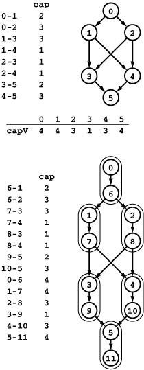
To solve the problem of finding a maxflow in the network at the top such that flow through each vertex does not exceed the capacity bound given in the vertex-indexed array capV, we build the standard network at the bottom: Associate a new vertex u* (where u* denotes u+V) with each vertex u, add an edge u-u* whose capacity is the capacity of u, and include an edge u*-v for each edge u-v. Each u-u* pair is encircled in the diagram. Any flow in the bottom network corresponds directly to a flow in the top network that satisfies the vertex-capacity constraints.

Allowing multiple sinks and sources or adding capacity constraints seem to generalize the maxflow problem; the interest of Properties 22.14 and 22.15 is that these problems are actually no more difficult than the standard problem. Next, we consider a version of the problem that might seem to be easier to solve.

Acyclic networks Find a maxflow in an acyclic network. Does the presence of cycles in a flow network make more difficult the task of computing a maxflow?

We have seen many examples of digraph-processing problems that are much more difficult to solve in the presence of cycles. Perhaps the most prominent example is the shortest-paths problem in weighted digraphs with edge weights that could be negative (see Section 21.7), which is simple to solve in linear time if there are no cycles but NP-complete if cycles are allowed. But the maxflow problem, remarkably, is no easier for acyclic networks.

Property 22.16 The maxflow problem for acyclic networks is equivalent to the standard maxflow problem.

Proof: Again, we need only to show that the standard problem reduces to the acyclic problem. Given any network with V vertices and E edges, we construct a network with 2V +2 vertices and E +3V edges that is not just acyclic but has a simple structure.

Let u* denote u+V, and build a bipartite digraph consisting of two vertices u and u* corresponding to each vertex u in the original network and one edge u-v* corresponding to each edge u-v in the original network with the same capacity. Now, add to the bipartite digraph a source s and a sink t and, for each vertex u in the original graph, an edge s-u and an edge u*-t, both of capacity equal to the sum of the capacities of u’s outgoing edges in the original network. Also, let X be the sum of the capacities of the edges in the original network, and add edges from u to u*, with capacity X +1. This construction is illustrated in Program 22.33.

Figure 22.33 Reduction to acyclic network

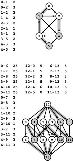
Each vertex u in the top network corresponds to two vertices u and u* (where u* denotes u+V) in the bottom network and each edge u-v in the top network corresponds to an edge u-v* in the bottom network. Additionally, the bottom network has uncapacitated edges u-u*, a source s with an edge to each unstarred vertex, and a sink t with an edge from each starred vertex. The shaded and un-shaded vertices (and edges which connect shaded to unshaded) illustrate the direct relationship among cuts in the two networks (see text).

To show that any maxflow in the original network corresponds to a maxflow in the transformed network, we consider cuts rather than flows. Given any st-cut of size c in the original network, we show how to construct an st-cut of size c+ X in the transformed network; and, given any minimal st-cut of size c+ X in the transformed network, we show how to construct an st-cut of size c in the original network. Thus, given a minimal cut in the transformed network, the corresponding cut in the original network is minimal. Moreover, our construction gives a flow whose value is equal to the minimal-cut capacity, so it is a maxflow.

Given any cut of the original network that separates the source from the sink, let S be the source’s vertex set and T the sink’s vertex set. Construct a cut of the transformed network by putting vertices in S in a set with s and vertices in T in a set with t and putting u and u* on the same side of the cut for all u, as illustrated in Program 22.33. For every u, either s-u or P|u*-t| is in the cut set, and u-v* is in the cut set if and only if u-v is in the cut set of the original network; so the total capacity of the cut is equal to the capacity of the cut in the original network plus X.

Given any minimal st-cut of the transformed network, let S* be s’s vertex set and T*t’s vertex set. Our goal is to construct a cut of the same capacity with u and u* both in the same cut vertex set for all u so that the correspondence of the previous paragraph gives a cut in the original network, completing the proof. First, if u is in S and u* in T*, then u-u* must be a crossing edge, which is a contradiction: u-u* cannot be in any minimal cut, because a cut consisting of all the edges corresponding to the edges in the original graph is of lower cost. Second, if u is in T and u* is in S, then s-u must be in the cut, because that is the only edge connecting s to u. But we can create a cut of equal cost by substituting all the edges directed out of u for s-u, moving u to S*.

Given any flow in the transformed network of value c + X, we simply assign the same flow value to each corresponding edge in the original network to get a flow with value c. The cut transformation at the end of the previous paragraph does not affect this assignment, because it manipulates edges with flow value zero.

The result of the reduction not only is an acyclic network, but also has a simple bipartite structure. The reduction says that we could, if we wished, adopt these simpler networks, rather than general networks, as our standard. It would seem that perhaps this special structure would lead to faster maxflow algorithms. But the reduction shows that we could use any algorithm that we found for these special acyclic networks to solve maxflow problems in general networks, at only modest extra cost. Indeed, the classical maxflow algorithms exploit the flexibility of the general network model: Both the augmenting-path and preflow-push approaches that we have considered use the concept of a residual network, which involves introducing cycles into the network.

Figure 22.34 Reduction from undirected networks

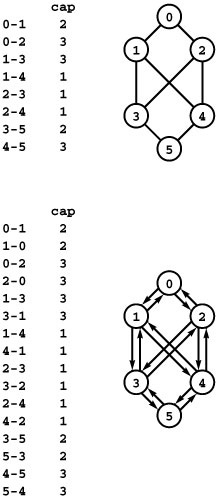
To solve a maxflow problem in an undirected network, we can consider it to be a directed network with edges in each direction. Note that the residual network for such a network has four edges corresponding to each edge in the undirected network.

When we have a maxflow problem for an acyclic network, we typically use the standard algorithm for general networks to solve it.

The construction of Property 22.16 is elaborate, and it illustrates that reduction proofs can require care, if not ingenuity. Such proofs are important because not all versions of the maxflow problem are equivalent to the standard problem, and we need to know the extent of the applicability of our algorithms. Researchers continue to explore this topic because reductions relating various natural problems have not yet been established, as illustrated by the following example.

Maxflow in undirected networks An undirected flow network is a weighted graph with integer edge weights that we interpret to be capacities. A circulation in such a network is an assignment of weights and directions to the edges satisfying the conditions that the flow on each edge is no greater than that edge’s capacity and that the total flow into each vertex is equal to the total flow out of that vertex. The undirected maxflow problem is to find a circulation that maximizes the flow in specified direction in a specified edge (that is, from some vertex s to some other vertex t). This problem perhaps corresponds more naturally than the standard problem to our liquid-flowing-through-pipes model: It corresponds to allowing liquid to flow through a pipe in either direction.

Property 22.17 The maxflow problem for undirected st-networks reduces to the maxflow problem for st-networks.

Proof: Given an undirected network, construct a directed network with the same vertices and two directed edges corresponding to each edge, one in each direction, both with the capacity of the undirected edge. Any flow in the original network certainly corresponds to a flow with the same value in the transformed network. The converse is also true: If u-v has flow f and v-u flow g in the undirected network, then we can put the flow f − g in u-v in the directed network if f≥g; g −f in v-u otherwise. Thus, any maxflow in the directed network is a maxflow in the undirected network: The construction gives a flow, and any flow with a higher value in the directed network would correspond to some flow with a higher value in the undirected network; but no such flow exists.

This proof does not establish that the problem for undirected networks is equivalent to the standard problem. That is, it leaves open

Figure 22.35 Feasible flow

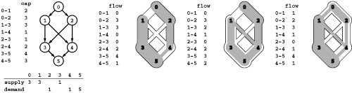
In a feasible-flow problem, we specify supply and demand constraints at the vertices in addition to the capacity constraints on the edges. We seek any flow for which outflow equals supply plus inflow at supply vertices and inflow equals outflow plus demand at demand vertices. Three solutions to the feasible-flow problem at left are shown on the right.

the possibility that finding maxflows in undirected networks is easier than finding maxflows in standard networks (see Exercise 22.81).

In summary, we can handle networks with multiple sinks and sources, undirected networks, networks with capacity constraints on vertices, and many other types of networks (see, for example, Exercise 22.79) with the maxflow algorithms for st-networks in the previous two sections. In fact, Property 22.16 says that we could solve all these problems with even an algorithm that works for only acyclic networks.

Next, we consider a problem that is not an explicit maxflow problem but that we can reduce to the maxflow problem and therefore solve with maxflow algorithms. It is one way to formalize a basic version of the merchandise-distribution problem described at the beginning of this chapter.

Feasible flow Suppose that a weight is assigned to each vertex in a flow network, and is to be interpreted as supply (if positive) or demand (if negative), with the sum of the vertex weights equal to zero. Define a flow to be feasible if the difference between each vertex’s outflow and inflow is equal to that vertex’s weight (supply if positive and demand if negative). Given such a network, determine whether or not a feasible flow exists. Program 22.35 illustrates a feasible-flow problem.

Supply vertices correspond to warehouses in the merchandise-distribution problem; demand vertices correspond to retail outlets; and edges correspond to roads on the trucking routes. The feasible-flow problem answers the basic question of whether it is possible to find a way to ship the goods such that supply meets demand everywhere.

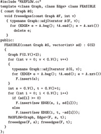
Figure 22.36 Reduction from feasible flow

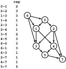
This network is a standard network constructed from the feasible-flow problem in Program 22.35 by adding edges from a new source vertex to the supply vertices (each with capacity equal to the amount of the supply) and edges to a new sink vertex from the demand vertices (each with capacity equal to the amount of the demand). The network in Program 22.35 has a feasible flow if and only if this network has a flow (a maxflow) that fills all the edges from the sink and all the edges to the source.

Property 22.18 The feasible-flow problem reduces to the maxflow problem.

Proof: Given a feasible-flow problem, construct a network with the same vertices and edges but with no weights on the vertices. Instead, add a source vertex s that has an edge to each supply vertex with weight equal to that vertex’s supply and a sink vertex t that has an edge from each demand vertex with weight equal to the negation of that vertex’s demand (so that the edge weight is positive). Solve the maxflow problem on this network. The original network has a feasible flow if and only if all the edges out of the source and all the edges into the sink are filled to capacity in this flow. Program 22.36 illustrates an example of this reduction.

Developing classes that implement reductions of the type that we have been considering can be a challenging software-engineering task, primarily because the objects that we are manipulating are represented with complicated data structures. To reduce another problem to a standard maxflow problem, should we create a new network? Some of the problems require extra data, such as vertex capacities or supply and demand, so creating a standard network without these data might be justified. Our use of edge pointers plays a critical role here: If we copy a network’s edges and then compute a maxflow, what are we to do with the result? Transferring the computed flow (a weight on each edge) from one network to another when both are represented with adjacency lists is not a trivial computation. With edge pointers, the new network has copies of pointers, not edges, so we can transfer flow assignments right through to the client’s network. Program 22.6 is an implementation that illustrates some of these considerations in a class for solving feasible-flow problems using the reduction of Property 22.16.

A canonical example of a flow problem that we cannot handle with the maxflow model, and that is the subject of Sections 22.5 and 22.6, is an extension of the feasible-flow problem. We add a second set of edge weights that we interpret as costs, define flow costs in terms of these weights, and ask for a feasible flow of minimal cost. This model formalizes the general merchandise-distribution problem. We are interested not just in whether it is possible to move the goods but also in what is the lowest-cost way to move them.

All the problems that we have considered so far in this section have the same basic goal (computing a flow in a flow network), so it is perhaps not surprising that we can handle them with a flow-network problem-solving model. As we saw with the maxflow–mincut theorem, we can use maxflow algorithms to solve graph-processing problems that seem to have little to do with flows. We now turn to examples of this kind.

Maximum-cardinality bipartite matching Given a bipartite graph, find a set of edges of maximum cardinality such that each vertex is connected to at most one other vertex.

For brevity, we refer to this problem simply as the bipartite-matching problem except in contexts where we need to distinguish it from similar problems. It formalizes the job-placement problem discussed at the beginning of this chapter. Vertices correspond to individuals and employers; edges correspond to a “mutual interest in the job” relation. A solution to the bipartite-matching problem maximizes total employment. Program 22.37 illustrates the bipartite graph that models the example problem in Program 22.3.

Figure 22.37 Bipartite matching

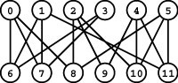
This instance of the bipartite-matching problem formalizes the job-placement example depicted in Program 22.3. Finding the best way to match the students to the jobs in that example is equivalent to finding the maximum number of vertex-disjoint edges in this bipartite graph.

It is an instructive exercise to think about finding a direct solution to the bipartite-matching problem, without using the graph model. For example, the problem amounts to the following combinatorial puzzle: “Find the largest subset of a set of pairs of integers (drawn from disjoint sets) with the property that no two pairs have the same integer.” The example depicted in Program 22.37 corresponds to solving this puzzle on the pairs 0-6, 0-7, 0-8, 1-6, and so forth. The problem seems straightforward at first, but, as was true of the Hamilton-path problem that we considered in Section 17.7 (and many other problems), a naive approach that chooses pairs in some systematic way until finding a contradiction might require exponential time. That is, there are far too many subsets of the pairs for us to try all possibilities; a solution to the problem must be clever enough to examine only a few of them. Solving specific matching puzzles like the one just given or developing algorithms that can solve efficiently any such puzzle are nontrivial tasks that help to demonstrate the power and utility of the network-flow model, which provides a reasonable way to do bipartite matching.

Property 22.19 The bipartite-matching problem reduces to the maxflow problem.

Proof: Given a bipartite-matching problem, construct an instance of the maxflow problem by directing all edges from one set to the other, adding a source vertex with edges directed to all the members of one set in the bipartite graph, and adding a sink vertex with edge directed from all the members of the other set. To make the resulting digraph a network, assign each edge capacity 1. Program 22.38 illustrates this construction.

Now, any solution to the maxflow problem for this network provides a solution to the corresponding bipartite-matching problem. The matching corresponds exactly to those edges between vertices in the two sets that are filled to capacity by the maxflow algorithm. First, the network flow always gives a legal matching: Since each vertex has an edge of capacity one either coming in (from the sink) or going out (to the source), at most one unit of flow can go through each vertex, implying in turn that each vertex will be included at most once in the matching. Second, no matching can have more edges, since any such matching would lead directly to a better flow than that produced by the maxflow algorithm.

Figure 22.38 Reduction from bipartite matching

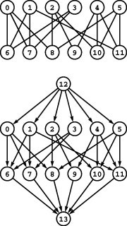
To find a maximum matching in a bipartite graph (top), we construct an st-network (bottom) by directing all the edges from the top row to the bottom row, adding a new source with edges to each vertex on the top row, adding a new sink with edges to each vertex on the bottom row, and assigning capacity 1 to all edges. In any flow, at most one outgoing edge from each vertex on the top row can be filled and at most one incoming edge to each vertex on the bottom row can be filled, so a solution to the maxflow problem on this network gives a maximum matching for the bipartite graph.

For example, in Program 22.38, an augmenting-path maxflow algorithm might use the paths s-0-6-t, s-1-7-t, s-2-8-t, s-4-9-t, s-5-10-t, and s-3-6-0-7-1-11-t to compute the matching 0-7, 1-11, 2-8, 3-6, 4-9, and 5-10. Thus, there is a way to match all the students to jobs in Program 22.3.

Program 22.7 is a client program that reads a bipartite-matching problem from standard input and uses the reduction described in this proof to solve it. What is the running time of this program for huge networks? Certainly, the running time depends on the maxflow algorithm and implementation that we use. Also, we need to take into account that the networks that we build have a special structure (unit-capacity bipartite flow networks)—not only do the running times of the various maxflow algorithms that we have considered not necessarily approach their worst-case bounds, but also we can substantially reduce the bounds. For example, the first bound that we considered, for the generic augmenting-path algorithm, provides a quick answer.

Corollary The time required to find a maximum-cardinality matching in a bipartite graph is O(V E).

Proof: Immediate from Property 22.6.

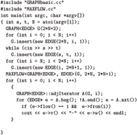
The operation of augmenting-path algorithms on unit-capacity bipartite networks is simple to describe. Each augmenting path fills one edge from the source and one edge into the sink. These edges are never used as back edges, so there are at most V augmenting paths. The V E upper bound holds for any algorithm that finds augmenting paths in time proportional to E.

Table 22.3 shows performance results for solving random bipartite-matching problems using various augmenting-path algorithms. It is clear from this table that actual running times for this problem are closer to the V E worst case than to the optimal (linear)

Table 22.3 Empirical study for bipartite matching

This table shows performance parameters (number of vertices expanded and number of adjacency-list nodes touched) when various augmenting-path maxflow algorithms are used to compute a maximum bipartite matching for graphs with 2000 pairs of vertices and 500 edges (top) and 4000 edges (bottom). For this problem, depth-first search is the most effective method.

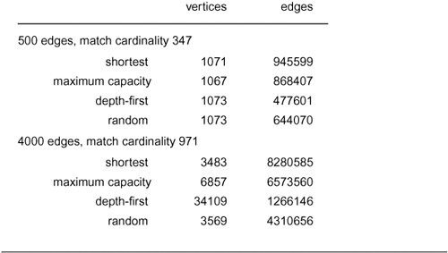
time. It is possible, with judicious choice and tuning of the maxflow implementation, to speed up this method by a factor of pV (see Exercises 22.91 and 22.92).

This problem is representative of a situation that we face more frequently as we examine new problems and more general problem-solving models, demonstrating the effectiveness of reduction as a practical problem-solving tool. If we can find a reduction to a known general model such as the maxflow problem, we generally view that as a major step toward developing a practical solution, because it at least indicates not only that the problem is tractable, but also that we have numerous efficient algorithms for solving the problem. In many situations, it is reasonable to use an existing maxflow class to solve the problem and move on to the next problem. If performance remains a critical issue, we can study the relative performance of various maxflow algorithms or implementations, or we can use their behavior as the starting point to develop a better, special-purpose algorithm.

The general problem-solving model provides both an upper bound that we can choose either to live with or to strive to improve, and a host of implementations that have proved effective on a variety of other problems.

Next, we discuss problems relating to connectivity in graphs. Before considering the use of maxflow algorithms to solve connectivity problems, we examine the use of the maxflow–mincut theorem to take care of a piece of unfinished business from Chapter 18: The proofs of the basic theorems relating to paths and cuts in undirected graphs. These proofs are further testimony to the fundamental importance of the maxflow–mincut theorem.

Property 22.20 (Menger’s Theorem) The minimum number of edges whose removal disconnects two vertices in a digraph is equal to the maximum number of edge-disjoint paths between the two vertices.

Proof: Given a digraph, define a flow network with the same vertices and edges with all edge capacities defined to be 1. By Property 22.2, we can represent any st-flow as a set of edge-disjoint paths from s to t, with the number of such paths equal to the value of the flow. The capacity of any st-cut is equal to that cut’s cardinality. Given these facts, the maxflow–mincut theorem implies the stated result.

The corresponding results for undirected graphs, and for vertex connectivity for digraphs and for undirected graphs, involve reductions similar to those considered here and are left for exercises (see Exercises 22.94 through 22.96).

Now we turn to algorithmic implications of the direct connection between flows and connectivity that is established by the maxflow– mincut theorem. Property 22.5 is perhaps the most important algorithmic implication (the mincut problem reduces to the maxflow problem), but the converse is not known to be true (see Exercise 22.47). Intuitively, it seems as though knowing a mincut should make easier the task of finding a maxflow, but no one has been able to demonstrate how. This basic example highlights the need to proceed with care when working with reductions among problems.

Still, we can also use maxflow algorithms to handle numerous connectivity problems. For example, they help solve the first nontrivial graph-processing problems that we encountered, in Chapter 18.

Edge connectivity What is the minimum number of edges that need to be removed to separate a given graph into two pieces? Find a set of edges of minimal cardinality that does this separation.

Vertex connectivity What is the minimum number of vertices that need to be removed to separate a given graph into two pieces? Find a set of vertices of minimal cardinality that does this separation.

These problems also are relevant for digraphs, so there are a total of four problems to consider. As with Menger’s theorem, we consider one of them in detail (edge connectivity in undirected graphs) and leave the others for exercises.

Property 22.21 The time required to determine the edge connectivity of an undirected graph is O(E²).

Proof: We can compute the minimum size of any cut that separates two given vertices by computing the maxflow in the st-network formed from the graph by assigning unit capacity to each edge. The edge connectivity is equal to the minimum of these values over all pairs of vertices.

We do not need to do the computation for all pairs of vertices, however. Let s* be a vertex of minimal degree in the graph. Note that the degree of s* can be no greater than 2E/V. Consider any minimum cut of the graph. By definition, the number of edges in the cut set is equal to the graph’s edge connectivity. The vertex s* appears in one of the cut’s vertex sets, and the other set must have some vertex t, so the size of any minimal cut separating s* and t must be equal to the graph’s edge connectivity. Therefore, if we solve V-1 maxflow problems (using s* as the source and each other vertex as the sink), the minimum flow value found is the edge connectivity of the network.

Now, any augmenting-path maxflow algorithm with s* as the source uses at most 2E/V paths; so, if we use any method that takes at most E steps to find an augmenting path, we have a total of at most (V − 1)(2E/V )E steps to find the edge connectivity and that implies the stated result.

This method, unlike all the other examples of this section, is not a direct reduction of one problem to another, but it does give a practical algorithm for computing edge connectivity. Again, with a careful maxflow implementation tuned to this specific problem, we can improve performance—it is possible to solve the problem in time proportional to V E (see reference section). The proof of Property 22.21 is an example of the more general concept of efficient (polynomial-time) reductions that we first encountered in Section 21.7 and that plays an essential role in the theory of algorithms discussed in Part 8. Such a reduction both proves the problem to be tractable and provides an algorithm for solving it—significant first steps in coping with a new combinatorial problem.

We conclude this section by considering a strictly mathematical formulation of the maxflow problem, using linear programming (LP) (see Section 21.6). This exercise is useful because it helps us to see relationships to other problems that can be so formulated.

The formulation is straightforward: We consider a system of inequalities that involve one variable corresponding to each edge, two inequalities corresponding to each edge, and one equation corresponding to each vertex. The value of the variable is the edge flow, the inequalities specify that the edge flow must be between 0 and the edge’s capacity, and the equations specify that the total flow on the edges that go into each vertex must be equal to the total flow on the edges that go out of that vertex.

Figure 22.39 LP formulation of a maxflow problem

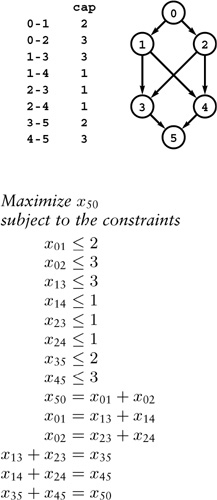
This linear program is equivalent to the maxflow problem for the sample network of Program 22.5. There is one inequality for each edge (which specifies that flow cannot exceed capacity) and one equality for each vertex (which specifies that flow in must equal flow out). We use a dummy edge from sink to source to capture the flow in the network, as described in the discussion following Property 22.2.

Figure 22.39 illustrates an example of this construction. Any maxflow problem can be cast as a LP problem in this way. LP is a versatile approach to solving combinatorial problems, and a great number of the problems that we study can be formulated as linear programs. The fact that maxflow problems are easier to solve than LP problems may be explained by the fact that the constraints in the LP formulation of maxflow problems have a specific structure not necessarily found in all LP problems.

Even though the LP problem is much more difficult in general than are specific problems such as the maxflow problem, there are powerful algorithms that can solve LP problems efficiently. The worst-case running time of these algorithms certainly exceeds the worst-case running of the specific algorithms that we have been considering, but an immense amount of practical experience over the past several decades has shown them to be effective for solving problems of the type that arise in practice.

The construction illustrated in Program 22.39 indicates a proof that the maxflow problem reduces to the LP problem, unless we insist that flow values be integers. When we examine LP in detail in Part 8, we describe a way to overcome the difficulty that the LP formulation does not carry the constraint that the results have integer values.

This context gives us a precise mathematical framework that we can use to address ever more general problems and to create ever more powerful algorithms to solve those problems. The maxflow problem is easy to solve and also is versatile in its own right, as indicated by the examples in this section. Next, we examine a harder problem (still easier than LP) that encompasses a still-wider class of practical problems. We discuss ramifications of building solutions to these increasingly general problem-solving models at the end of this chapter, setting the stage for a full treatment in Part 8.

Exercises

• 22.70 Define a class for finding a circulation with maximal flow in a specified edge. Provide an implementation that uses MAXFLOW.

22.71 Define a class for finding a maxflow in a network with no constraint on the number of sources or sinks. Provide an implementation that uses MAXFLOW.

22.72 Define a class for finding a maxflow in an undirected network. Provide an implementation that uses MAXFLOW.

22.73 Define a class for finding a maxflow in a network with capacity constraints on vertices. Provide an implementation that uses MAXFLOW.

• 22.74 Develop a class for feasible-flow problems that includes member functions allowing clients to set supply–demand values and to check that flow values are properly related at each vertex.

22.75 Do Exercise 22.18 for the case that each distribution point has limited capacity (that is, there is a limit on the amount of goods that can be stored there at any given time).

• 22.76 Show that the maxflow problem reduces to the feasible-flow problem (so that the two problems are therefore equivalent).

22.77 Find a feasible flow for the flow network shown in Program 22.10, given the additional constraints that 0, 2, and 3 are supply vertices with weight 4, andthat 1, 4, and 5 are supply vertices with weights 1, 3, and 5, respectively.

• 22.78 Write a program that takes as input a sports league’s schedule and current standings and determines whether a given team is eliminated. Assume that there are no ties. Hint: Reduce to a feasible-flow problem with one source node that has a supply value equal to the total number of games remaining to play in the season, sink nodes that correspond to each pair of teams having a demand value equal to the number of remaining games between that pair, and distribution nodes that correspond to each team. Edges should connect the supply node to each team’s distribution node (of capacity equal to the number of games that team would have to win to beat X if X were to win all its remaining games), and there should be an (uncapacitated) edge connecting each team’s distribution node to each of the demand nodes involving that team.

• 22.79 Prove that the maxflow problem for networks with lower bounds on edges reduces to the standard maxflow problem.

• 22.80 Prove that, for networks with lower bounds on edges, the problem of finding a minimal flow (that respects the bounds) reduces to the maxflow problem (see Exercise 22.79).

••• 22.81 Prove that the maxflow problem for st-networks reduces to the maxflow problem for undirected networks, or find a maxflow algorithm for undirected networks that has a worst-case running time substantially better than those of the algorithms in Sections 22.2 and 22.3.

• 22.82 Find all the matchings with five edges for the bipartite graph in Program 22.37.

22.83 Extend Program 22.7 to use symbolic names instead of integers to refer to vertices (see Program 17.10).

• 22.84 Prove that the bipartite-matching problem is equivalent to the problem of finding maxflows in networks where all edges are of unit capacity.

22.85 We might interpret the example in Program 22.3 as describing student preferences for jobs and employer preferences for students, the two of which may not be mutual. Does the reduction described in the text apply to the directed bipartite-matching problem that results from this interpretation, where edges in the bipartite graph are directed (in either direction) from one set to the other? Prove that it does or provide a counterexample.

• 22.86 Construct a family of bipartite-matching problems where the average length of the augmenting paths used by any augmenting-path algorithm to solve the corresponding maxflow problem is proportional to E.

22.87 Show, in the style of Program 22.28, the operation of the FIFO preflow-push network-flow algorithm on the bipartite-matching network shown in Program 22.38.

• 22.88 Extend Table 22.3 to include various preflow-push algorithms.

•• 22.89 Suppose that the two sets in a bipartite-matching problem are of size S and T, with S << T. Give as sharp a bound as you can for the worst-case running time to solve this problem, for the reduction of Property 22.19 and the maximal-augmenting-path implementation of the Ford–Fulkerson algorithm (see Property 22.8).

• 22.90 Exercise 22.89 for the FIFO-queue implementation of the preflow-push algorithm (see Property 22.13).

22.91 Extend Table 22.3 to include implementations that use the all-augmenting-paths approach described in Exercise 22.37.

•• 22.92 Prove p that the running time of the method described in Exercise 22.91 is O(E) for BFS.

22.93 Do empirical studies to plot the expected number of edges in a maximal matching in random bipartite graphs with V + V vertices and E edges, for a reasonable set of values for V and sufficient values of E to plot a smooth curve that goes from zero to V.

• 22.94 Prove Menger’s theorem (Property 22.20) for undirected graphs.

• 22.95 Prove that the minimum number of vertices whose removal disconnects two vertices in a digraph is equal to the maximum number of vertex-disjoint paths between the two vertices. Hint: Use a vertex-splitting transformation, similar to the one illustrated in Program 22.32.

• 22.96 Extend your proof for Exercise 22.95 to apply to undirected graphs.

22.97 Implement an edge-connectivity class for the graph ADT of Chapter 17 whose constructor uses the algorithm described in this section to support a public member function that returns the graph’s connectivity.

22.98 Extend your solution to Exercise 22.97 to put in a user-supplied vector a minimal set of edges that separates the graph. How big a vector should the user expect?

• 22.99 Develop an algorithm for computing the edge connectivity of di-graphs (the minimal number of edges whose removal leaves a digraph that is not strongly connected). Implement a class based on your algorithm for the digraph ADT of Chapter 19.

• 22.100 Develop algorithms based on your solutions to Exercises 22.95 and 22.96 for computing the vertex connectivity of digraphs and undirected graphs. Implement classes based on your algorithms for the digraph ADT of Chapter 19 and the graph ADT of Chapter 17, respectively (see Exercises 22.97 and 22.98).

22.101 Describe how to find the vertex connectivity of a digraph by solving V lg V unit-capacity maxflow problems. Hint: Use Menger’s theorem and binary search.

• 22.102 Run empirical studies based on your solution to Exercise 22.97 to determine edge connectivity of various graphs (see Exercises 17.63–76).

• 22.103 Give an LP formulation for the problem of finding a maxflow in the flow network shown in Program 22.10.

• 22.104 Formulate as an LP problem the bipartite-matching problem in Program 22.37.

22.5 Mincost Flows

It is not unusual for there to be numerous solutions to a given maxflow problem. This fact leads to the question of whether we might wish to impose some additional criteria for choosing one of them. For example, there are clearly many solutions to the unit-capacity flow problems shown in Program 22.22; perhaps we would prefer the one that uses the fewest edges or the one with the shortest paths, or perhaps we would like to know whether there exists one comprising disjoint paths. Such problems are more difficult than the standard maxflow problem; they fall into a more general model known as the mincost flow problem, which is the subject of this section.

As with the maxflow problem, there are numerous equivalent ways to pose the mincost-flow problem. We consider one standard formulation in detail in this section, then consider various reductions in Section 22.7.

Specifically, we use the mincost-maxflow model: We define an edge type that includes integer costs, use the edge costs to define a flow cost in a natural way, then ask for a maximal flow of minimal cost. As we learn, not only do we have efficient and effective algorithms for this problem, but also the problem-solving model is of broad applicability.

Definition 22.8 The flow cost of an edge in a flow network with edge costs is the product of that edge’s flow and cost. The cost of a flow is the sum of the flow costs of that flow’s edges.

We continue to assume that capacities are positive integers less than M. We also assume edge costs to be nonnegative integers less than C. (Disallowing negative costs is primarily a matter of convenience, as discussed in Section 22.7.) As before, we assign names to these upper-bound values because the running times of some algorithms depend on the latter. With these basic assumptions, the problem that we wish to solve is trivial to define.

Mincost maxflow Given a flow network with edge costs, find a maxflow such that no other maxflow has lower cost.

Figure 22.40 illustrates different maxflows in a flow network with costs, including a mincost maxflow. Certainly, the computational burden of minimizing cost is no less challenging than the burden of maximizing flow with which we were concerned in Sections 22.2

Figure 22.40 Maxflows in flow networks with costs

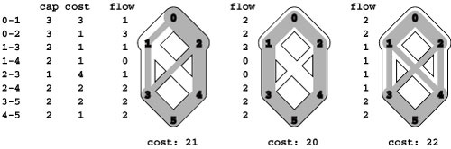
These flows all have the same (maximal) value, but their costs (the sum of the products of edge flows and edge costs) differ. The maxflow in the center has minimal cost (no maxflow has lower cost).

and 22.3. Indeed, costs add an extra dimension that presents significant new challenges. Even so, we can shoulder this burden with a generic algorithm that is similar to the augmenting-path algorithm for the maxflow problem.

Numerous other problems reduce to or are equivalent to the mincost-maxflow problem. For example, the following formulation is of interest because it encompasses the merchandise-distribution problem that we considered at the beginning of the chapter.

Mincost feasible flow Recall that we define a flow in a network with vertex weights (supply if positive, demand if negative) to be feasible if the sum of the vertex weights is negative and the difference between each vertex’s outflow and inflow. Given such a network, find a feasible flow of minimal cost.

To describe the network model for the mincost–feasible-flow problem, we use the term distribution network for brevity to mean “capacitated flow network with edge costs and supply or demand weights on vertices.”

In the merchandise-distribution application, supply vertices correspond to warehouses, demand vertices to retail outlets, edges to trucking routes, supply or demand values to the amount of material to be shipped or received, and edge capacities to the number and capacity of the trucks available for the various routes. A natural way to interpret each edge’s cost is as the cost of moving a unit of flow through that edge (the cost of sending a unit of material in a truck along the corresponding route). Given a flow, an edge’s flow cost is the part of the cost of moving the flow through the network that we can attribute to that edge. Given an amount of material that is to be shipped along a given edge, we can compute the cost of shipping it by multiplying the cost per unit by the amount. Doing this computation for each edge

and adding the results together gives us the total shipping cost, which we would like to minimize.

Property 22.22 The mincost–feasible-flow problem and the mincostmaxflow problems are equivalent.

Proof: Immediate, by the same correspondence as Property 22.18 (see also Exercise 22.76).

Because of this equivalence and because the mincost–feasible-flow problem directly models merchandise-distribution problems and many other applications, we use the term mincost flow to refer to both problems in contexts where we could refer to either. We consider other reductions in Section 22.7.

To implement edge costs in flow networks, we add an integer pcost private data member to the EDGE class from Section 22.1 and a member function cost() to return its value to clients. Program 22.8 is a client function that computes the cost of a flow in a graph built with pointers to such edges. As when we work with maxflows, it is also prudent to implement a function to check that inflow and outflow values are properly related at each vertex and that the data structures are consistent (see Exercise 22.12).

The first step in developing algorithms to solve the mincost-flow problem is to extend the definition of residual networks to include costs on the edges.

Definition 22.9 Given a flow in a flow network with edge costs, the residual network for the flow has the same vertices as the original and one or two edges in the residual network for each edge in the original, defined as follows: For each edge u-v in the original, let f be the flow, c the capacity, and x the cost. If f is positive, include an edge v-u in the residual with capacity f and cost-x; if f is less than c , include an edge u-v in the residual with capacity c-f and cost x.

This definition is nearly identical to Definition 22.4, but the difference is crucial. Edges in the residual network that represent backward edges have negative cost. To implement this convention, we use the following member function in the edge class:

int costRto(int v)
 { return from(v) ? -pcost : pcost; }

Traversing backward edges corresponds to removing flow in the corresponding edge in the original network, so the cost has to be reduced accordingly. Because of the negative edge costs, these networks can have negative-cost cycles. The concept of negative cycles, which seemed artificial when we first considered it in the context of shortest-paths algorithms, plays a critical role in mincost-flow algorithms, as we now see. We consider two algorithms, both based on the following optimality condition.

Property 22.23 A maxflow is a mincost maxflow if and only if its residual network contains no negative-cost (directed) cycle.

Proof: Suppose that we have a mincost maxflow whose residual network has a negative-cost cycle. Let x be the capacity of a minimal-capacity edge in the cycle. Augment the flow by adding x to edges in the flow corresponding to positive-cost edges in the residual network (forward edges) and subtracting x from edges corresponding to negative-cost edges in the residual network (backward edges). These changes do not affect the difference between inflow and outflow at any vertex, so the flow remains a maxflow, but they change the network’s cost by x times the cost of the cycle, which is negative, thereby contradicting the assertion that the cost of the original flow was minimal.

To prove the converse, suppose that we have a maxflow F with no negative-cost cycles whose cost is not minimal, and con- sider any mincost maxflow M. By an argument identical to the flow-decomposition theorem (Property 22.2), we can find at most E directed cycles such that adding those cycles to the flow F gives the flow M. But, since F has no negative cycles, this operation cannot lower the cost of F, a contradiction. In other words, we should be able to convert F to M by augmenting along cycles, but we cannot do so because we have no negative-cost cycles to use to lower the flow cost.

This property leads immediately to a simple generic algorithm for solving the mincost-flow problem, called the cycle-canceling algorithm.

This method brings together machinery that we have developed over this chapter and the previous one to provide effective algorithms for solving the wide class of problems that fit into the mincost-flow model. Like several other generic methods that we have seen, it admits several different implementations, since the methods for finding the initial maxflow and for finding the negative-cost cycles are not specified. Figure 22.41 shows an example mincost-maxflow computation that uses cycle canceling.

Since we have already developed algorithms for computing a maxflow and for finding negative cycles, we immediately have the implementation of the cycle-canceling algorithm given in Program 22.9. We use any maxflow implementation to find the initial maxflow and the Bellman–Ford algorithm to find negative cycles (see Exercise 22.108). To these two implementations, we need to add only a loop to augment flow along the cycles.

We can eliminate the initial maxflow computation in the cycle-canceling algorithm by adding a dummy edge from source to sink and assigning to it a cost that is higher than the cost of any source–sink path in the network (for example, VC ) and a flow that is higher than the maxflow (for example, higher than the source’s outflow). With this initial setup, cycle canceling moves as much flow as possible out of the dummy edge, so the resulting flow is a maxflow. A mincost-flow computation using this technique is illustrated in Program 22.42. In the figure, we use an initial flow equal to the maxflow to make plain that the algorithm is simply computing another flow of the same value but

Figure 22.41 Residual networks (cycle canceling)

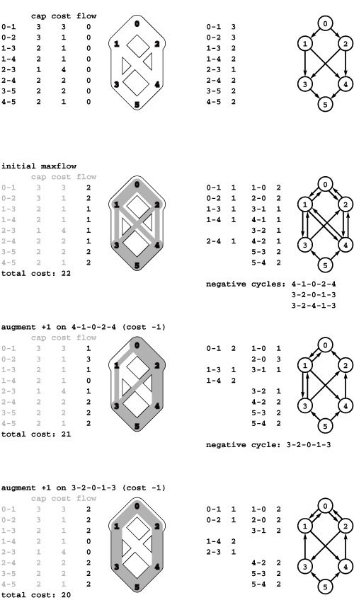
Each of the flows depicted here is a maxflow for the flow network depicted at the top, but only the one at the bottom is a mincost maxflow. To find it, we start with any maxflow and augment flow around negative cycles. The initial maxflow (second from top) has a cost of 22, which is not a min-cost maxflow because the residual network (shown at right) has three negative cycles. In this example, we augment along 4-1-0-2-4 to get a maxflow of cost 21 (third from top), which still has one negative cycle. Augmenting along that cycle gives a mincost flow (bottom). Note that augmenting along 3-2-4-1-3 in the first step would have brought us to the mincost flow in one step.

lower cost (in general, we do not know the flow value, so there is some flow left in the dummy edge at the end, which we ignore). As is evident from the figure, some augmenting cycles include the dummy edge and increase flow in the network; others do not include the dummy edge and reduce cost. Eventually, we reach a maxflow; at that point, all the augmenting cycles reduce cost without changing the value of the flow, as when we started with a maxflow.

Technically, using a dummy-flow initialization is neither more nor less generic than using a maxflow initialization for cycle canceling. The former does encompass all augmenting-path maxflow algorithms, but not all maxflows can be computed with an augmenting-path algorithm

Figure 22.42 Cycle canceling without initial maxflow

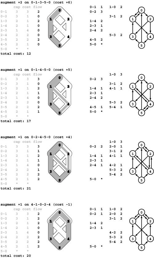
This sequence illustrates the computation of a mincost maxflow from an initially empty flow with the cycle-canceling algorithm by using a dummy edge from sink to source in the residual network with infinite capacity and infinite negative cost. The dummy edge makes any augmenting path from 0 to 5 a negative cycle (but we ignore it when augmenting and computing the cost of the flow). Augmenting along such a path increases the flow, as in augmenting-path algorithms (top three rows). When there are no cycles involving the dummy edge, there are no paths from source to sink in the residual network, so we have a maxflow (third from top). At that point, augmenting along a negative cycle decreases the cost without changing the flow value (bottom). In this example, we compute a maxflow, then decrease its cost; but that need not be the case. For example, the algorithm might have augmented along the negative cycle 1-4-5-3-1 instead of 0-1-4-5-0 in the second step. Since every augmentation either increases the flow or reduces the cost, we always wind up with a mincost maxflow.

(see Exercise 22.40). On the one hand, by using this technique, we may be giving up the benefits of a sophisticated maxflow algorithm; on the other hand, we may be better off reducing costs during the process of building a maxflow. In practice, dummy-flow initialization is widely used because it is so simple to implement.

As for maxflows, the existence of this generic algorithm guarantees that every mincost-flow problem (with capacities and costs that are integers) has a solution where flows are all integers; and the algorithm computes such a solution (see Exercise 22.107). Given this fact, it is easy to establish an upper bound on the amount of time that any cycle-canceling algorithm will require.

Property 22.24 The number of augmenting cycles needed in the generic cycle-canceling algorithm is less than ECM.

Proof: In the worst case, each edge in the initial maxflow has capacity M, cost C, and is filled. Each cycle reduces this cost by at least 1.

Corollary The time required to solve the mincost-flow problem in a sparse network is O(V³CM).

Proof: Immediate by multiplying the worst-case number of augmenting cycles by the worst-case cost of the Bellman–Ford algorithm for finding them (see Property 21.22).

Like that of augmenting-path methods, this running time is extremely pessimistic, as it assumes not only that we have a worst-case situation where we need to use a huge number of cycles to minimize cost, but also that we have another worst-case situation where we have to examine a huge number of edges to find each cycle. In many practical situations, we use relatively few cycles that are relatively easy to find, and the cycle-canceling algorithm is effective.

It is possible to develop a strategy that finds negative-cost cycles and ensures that the number of negative-cost cycles used is less than V E (see reference section). This result is significant because it establishes the fact that the mincost-flow problem is tractable (as are all the problems that reduce to it). However, practitioners typically use implementations that admit a bad worst case (in theory) but use substantially fewer iterations on the problems that arise in practice than predicted by the worst-case bounds.

The mincost-flow problem represents the most general problem-solving model that we have yet examined, so it is perhaps surprising that we can solve it with such a simple implementation. Because of the importance of the model, numerous other implementations of the cycle-canceling method and numerous other different methods have been developed and studied in detail. Program 22.9 is a remarkably simple and effective starting point, but it suffers from two defects that can potentially lead to poor performance. First, each time that we seek a negative cycle, we start from scratch. Can we save intermediate information during the search for one negative cycle that can help us find the next? Second, Program 22.9 just takes the first negative cycle that the Bellman–Ford algorithm finds. Can we direct the search towards negative cycles with particular properties? In Section 22.6, we consider an improved implementation, still generic, that represents a response to both of these questions.

Exercises

22.105 Expand your class for feasible flows from Exercise 22.74 to include costs. Use MINCOST to solves the mincost–feasible-flow problem.

• 22.106 Given a flow network whose edges are not all maximal capacity and cost, give an upper bound better than ECM on the cost of a maxflow.

22.107 Prove that, if all capacities and costs are integers, then the mincostflow problem has a solution where all flow values are integers.

22.108 Implement the negcyc() function for Program 22.9, using the Bellman-Ford algorithm (see Exercise 21.134).

• 22.109 Modify Program 22.9 to initialize with flow in a dummy edge instead of computing a flow.

• 22.110 Give all possible sequences of augmenting cycles that might have been depicted in Program 22.41.

• 22.111 Give all possible sequences of augmenting cycles that might have been depicted in Program 22.42.

22.112 Show, in the style of Program 22.41, the flow and residual networks after each augmentation when you use the cycle-canceling implementation of Program 22.9 to find a mincost flow in the flow network shown in Program 22.10, withcost 2 assigned to 0-2 and 0-3;cost 3 assigned to 2-5 and 3-5; cost 4 assigned to 1-4; and cost 1 assigned to all of the other edges. Assume that the maxflow is computed with the shortest-augmenting-path algorithm.

22.113 Answer Exercise 22.112, but assume that the program is modified to start with a maxflow in a dummy edge from source to sink, as in Program 22.42.

22.114 Extend your solutions to Exercises 22.6 and 22.7 to handle costs in flow networks.

22.115 Extend your solutions to Exercises 22.9 through 22.11 to include costs in the networks. Take each edge’s cost to be roughly proportional to the Euclidean distance between the vertices that the edge connects.

22.6 Network Simplex Algorithm

The running time of the cycle-canceling algorithm is based on not just the number of negative-cost cycles that the algorithm uses to reduce the flow cost but also the time that the algorithm uses to find each of the cycles. In this section, we consider a basic approach that both dramatically decreases the cost of identifying negative cycles and admits methods for reducing the number of iterations. This implementation of the cycle-canceling algorithm is known as the network simplex algorithm. It is based on maintaining a tree data structure and reweighting costs such that negative cycles can be identified quickly.

To describe the network simplex algorithm, we begin by noting that, with respect to any flow, each network edge u-v is in one of three states (see Figure 22.43):

Figure 22.43 Edge classification

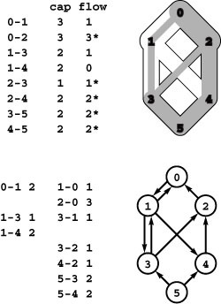
With respect to any flow, every edge is either empty, full, or partial (neither empty nor full). In this flow, edge 1-4 is empty; edges 0-2, 2-3, 2-4, 3-5, and 4-5 are full; and edges 0-1 and 1-3 are partial. Our conventions in figures give two ways to identify an edge’s state: In the flow column, 0 entries are empty edges; starred entries are full edges; and entries that are neither 0 nor starred are partial edges. In the residual network (bottom), empty edges appear only in the left column; full edges appear only in the right column; and partial edges appear in both columns.

• Empty, so flow can be pushed from only u to v

• Full, so flow can be pushed from only v to u

• Partial (neither empty nor full), so flow can pushed either way

This classification is familiar from our use of residual networks throughout this chapter. If u-v is an empty edge, then u-v is in the residual network, but v-u is not; if u-v is a full edge, then v-u is in the residual network, but u-v is not; if u-v is a partial edge, then both u-v and v-u are in the residual network.

Definition 22.10 Given a maxflow with no cycle of partial edges, a feasible spanning tree for the maxflow is any spanning tree of the network that contains all the flow’s partial edges.

In this context, we ignore edge directions in the spanning tree. That is, any set of V − 1 directed edges that connects the network’s V vertices (ignoring edge directions) constitutes a spanning tree, and a spanning tree is feasible if all nontree edges are either full or empty.

The first step in the network simplex algorithm is to build a spanning tree. One way to build it is to compute a maxflow, to break

Figure 22.44 Maxflow spanning tree

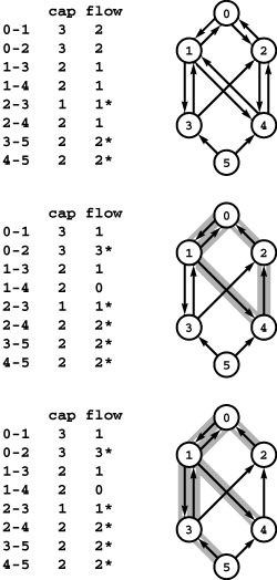
Given any maxflow (top), we can construct a maxflow that has a spanning tree such that no nontree edges are partial by the two-step process illustrated in this example. First, we break cycles of partial edges; in this case, we break the cycle 0-2-4-1-0 by pushing 1 unit of flow along it. We can always fill or empty at least one edge in this way; in this case, we empty 1-4 and fill both 0-2 and 2-4 (center). Second, we add empty or full edges to the set of partial edges to make a spanning tree; in this case, we add 0-2, 1-4 and 3-5 (bottom).

cycles of partial edges by augmenting along each cycle to fill or empty one of its edges, then to add full or empty edges to the remaining partial edges to make a spanning tree. An example of this process is illustrated in Program 22.44. Another option is to start with the maxflow in a dummy edge from source to sink. Then, this edge is the only possible partial edge, and we can build a spanning tree for the flow with any graph search. An example of such a spanning tree is illustrated in Program 22.45.

Now, adding any nontree edge to a spanning tree creates a cycle. The basic mechanism behind the network simplex algorithm is a set of vertex weights that allows immediate identification of the edges that, when added to the tree, create negative-cost cycles in the residual network. We refer to these vertex weights as potentials and use the notation ϕ (v) to refer to the potential associated with v. Depending on context, we refer to potentials as a function defined on the vertices, or as a set of integer weights with the implicit assumption that one is assigned to each vertex, or as a vertex-indexed vector (since we always store them that way in implementations).

Definition 22.11 Given a flow in a flow network with edge costs, let c (u, v)denote the cost of u-v in the flow’s residual network. For any potential function ϕ, the reduced cost of an edge u-v in the residual network with respect to ϕ, which we denote by c (u, v), is defined to be the value c(u, v)− (ϕ(u)− ϕ(v)).

In other words, the reduced cost of every edge is the difference between that edge’s actual cost and the difference of the potentials of the edge’s vertices. In the merchandise distribution application, we can see the intuition behind node potentials: If we interpret the potential ϕ (u) as the cost of buying a unit of material at node u, the full cost c (u, v)+ ϕ(u)− ϕ (v) is the cost of buying at u, shipping to v and selling at v.

We maintain a vertex-indexed vector phi for the vertex potentials and compute the reduced cost of an edge v-w by subtracting from the edge’s cost the value (phi[v] - phi[w]). That is, there is no need to store the reduced edge costs anywhere, because it is so easy to compute them.

In the network simplex algorithm, we use feasible spanning trees to define vertex potentials such that reduced edge costs with respect to those potentials give direct information about negative-cost cycles.

Figure 22.45 Spanning tree for dummy maxflow

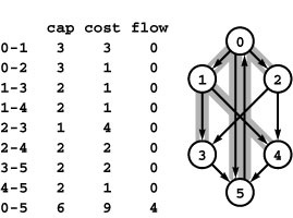
If we start with flow on a dummy edge from source to sink, then that is the only possible partial edge, so we can use any spanning tree of the remaining nodes to build a spanning tree for the flow. In the example, the edges 0-5, 0-1, 0-2, 1-3, and 1-4 comprise a spanning tree for the initial maxflow. All of the nontree edges are empty.

Specifically, we maintain a feasible spanning tree throughout the execution of the algorithm, and we set the values of the vertex potentials such that all tree edges have reduced cost zero.

Property 22.25 We say that a set of vertex potentials is valid with respect to a spanning tree if all tree edges have zero reduced cost. All valid vertex potentials for any given spanning tree imply the same reduced costs for each network edge.

Proof: Given two different potential functions ϕ and ϕ ^′ that are both valid with respect to a given spanning tree, we show that they differ by an additive constant: That ϕ (u) =ϕ ^′(u)+ ′for all u and some constant. Then, ϕ (u)−ϕ(v) =ϕ ^′(u)−ϕ^′(v) for all u and v, implying that all reduced costs are the same for the two potential functions.

For any two vertices u and v that are connected by a tree edge, we must have ϕ (v) =ϕ (u)c (u, v), by the following argument. If u-v is a tree edge, then ϕ (v) must − be equal to ϕ (u)c (u, v) to make the reduced cost c (u, v)− ϕ (u)+ ϕ (v) equal to zero; if v-u is a tree edge, then ϕ (v) must be equal to ϕ (u)+ c (v, u) =ϕ (u)c (u, v) to make the reduced cost c (v, u)− ϕ (v)+ ϕ (u) equal to zero. The same argument holds for ϕ ^′, so we must also have ϕ ^′(v) =ϕ ^′(u)c (u, v).

Subtracting, we find that ϕ (v)− ϕ ^′(v) =ϕ −(u)ϕ ^′(u) for any u and v connected by a tree edge. Denoting this difference by′ for any vertex and applying the equality along the edges of any search tree of the spanning tree immediately gives the desired result that ϕ(u) =ϕ ^′(u)+ ′for all u.

Another way to imagine the process of defining a set of valid vertex potentials is that we start by fixing one value, then compute the values for all vertices connected to that vertex by tree edges, then compute them for all vertices connected to those vertices, and so forth. No matter where we start the process, the potential difference between any two vertices is the same, determined by the structure of the tree. Program 22.46 depicts an example. We consider the details of the task of computing potentials after we examine the relationship between reduced costs on nontree edges and negative-cost cycles.

Property 22.26 We say that a nontree edge is eligible if the cycle that it creates with tree edges is a negative-cost cycle in the residual network. An edge is eligible if and only if it is a full edge with positive reduced cost or an empty edge with negative reduced cost.

Figure 22.46 Vertex potentials

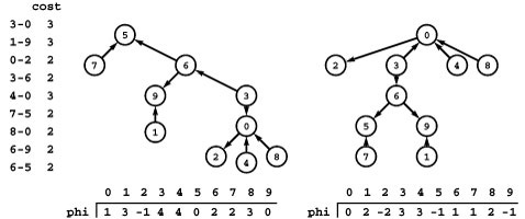
Vertex potentials are determined by the structure of the spanning tree and by an initial assignment of a potential value to any vertex. At left is a set of edges that comprise a spanning tree of the ten vertices 0 through 9. In the center is a representation of that tree with 5 at the root, vertices connected to 5 one level lower, and so forth. When we assign the root the potential value 0, there is a unique assignment of potentials to the other nodes that make the difference between the potentials of each edge’s vertices equal to its cost. At right is a different representation of the same tree with 0 at the root. The potentials that we get by assigning 0 the value 0 differ from those in the center by a constant offset. All our computations use the difference between two potentials: This difference is the same for any pair of potentials no matter what vertex we start with (and no matter what value we assign it), so our choice of starting vertex and value is immaterial.

Proof: Suppose that the edge u-v creates the cycle t1-t2-t3-…-td-t1 with tree edges t1-t2, t2-t3, …, where v is t1 and u is td. The reduced cost definitions of each edge imply the following:

c(u, v) = c (u, v)+ ϕ (u)− ϕ (t₁)
c(t₁,t₂) =ϕ (t₁)− ϕ (t₂)
c(t₂,t₃) =ϕ (t₂)ϕ (t₃)
.
.
.
c(t_d−1,u)= ϕ(t_d−1)− ϕ(u)

The left-hand side of the sum of these equations gives the total cost of the cycle, and the right-hand side collapses to c (u, v). In other words, the edge’s reduced cost gives the cycle cost, so only the edges described can give a negative-cost cycle

Property 22.27 If we have a flow and a feasible spanning tree with no eligible edges, the flow is a mincost flow.

Proof: If there are no eligible edges, then there are no negative-cost cycles in the residual network, so the optimality condition of Property 22.23 implies that the flow is a mincost flow.

An equivalent statement is that if we have a flow and a set of vertex potentials such that reduced costs of tree edges are all zero, full nontree edges are all nonnegative, and empty nontree edges are all nonpositive, then the flow is a mincost flow.

If we have eligible edges, we can choose one and augment along the cycle that it creates with tree edges to get a lower-cost flow. As we did with the cycle-canceling implementation in Section 22.5, we go through the cycle to find the maximum amount of flow that we can push, then go through the cycle again to push that amount, which fills or empties at least one edge. If that is the eligible edge that we used to create the cycle, it becomes ineligible (its reduced cost stays the same, but it switches from full to empty or empty to full). Otherwise, it becomes partial. By adding it to the tree and removing a full edge or an empty edge from the cycle, we maintain the invariant that no nontree edges are partial and that the tree is a feasible spanning tree. Again, we consider the mechanics of this computation later in this section.

In summary, feasible spanning trees give us vertex potentials, which give us reduced costs, which give us eligible edges, which give us negative-cost cycles. Augmenting along a negative-cost cycle reduces the flow cost and also implies changes in the tree structure. Changes in the tree structure imply changes in the vertex potentials; changes in the vertex potentials imply changes in reduced edge costs; and changes in reduced costs imply changes in the set of eligible edges. After making all these changes, we can pick another eligible edge and start the process again. This generic implementation of the cycle-canceling algorithm for solving the mincost-flow problem is called the network simplex algorithm.

This implementation is a generic one because the initial choice of spanning tree, the method of maintaining vertex potentials, and the method of choosing eligible edges are not specified. The strategy for choosing eligible edges determines the number of iterations, which trades off against the differing costs of implementing various strategies and recalculating the vertex potentials.

Property 22.28 If the generic network simplex algorithm terminates, it computes a mincost flow.

Proof: If the algorithm terminates, it does so because there are no negative-cost cycles in the residual network, so by Property 22.23 the maxflow is of mincost.

The condition that the algorithm might not terminate derives from the possibility that augmenting along a cycle might fill or empty multiple edges, thus leaving edges in the tree through which no flow can be pushed. If we cannot push flow, we cannot reduce the cost, and we could get caught in an infinite loop adding and removing edges to make a fixed sequence of spanning trees. Several ways to avoid this problem have been devised; we discuss them later in this section after we look in more detail at implementations.

The first choice that we face in developing an implementation of the network simplex algorithm is what representation to use for the spanning tree. We have three primary computational tasks that involve the tree:

• Computing the vertex potentials

• Augmenting along the cycle (and identifying an empty or a full edge on it)

• Inserting a new edge and removing an edge on the cycle formed Each of these tasks is an interesting exercise in data structure and algorithm design. There are several data structures and numerous algorithms that we might consider, with varied performance characteristics. We begin by considering perhaps the simplest available data structure—which we first encountered in Chapter 1(!)—the parent-link tree representation. After we examine algorithms and implementations that are based on the parent-link representation for the tasks just listed and describe their use in the context of the network simplex algorithm, we discuss alternative data structures and algorithms.

As we did in several other implementations in this chapter, beginning with the augmenting-path maxflow implementation, we keep links into the network representation, rather than simple indices in the tree representation, to allow us to have access to the flow values that need to be changed without losing access to the vertex name.

Program 22.10 is an implementation that assigns vertex potentials in time proportional to V. It is based on the following idea, also illustrated in Program 22.47. We start with any vertex and recursively compute the potentials of its ancestors, following parent links up to the root, to which, by convention, we assign potential 0. Then, we

pick another vertex and use parent links to compute recursively the potentials of its ancestors. The recursion terminates when we reach an ancestor whose potential is known; then, on the way out of the recursion, we travel back down the path, computing each node’s potential from its parent. We continue this process until we have computed all potential values. Once we have traveled along a path, we do not revisit any of its edges, so this process runs in time proportional to V.

Given two nodes in a tree, their least common ancestor (LCA) is the root of the smallest subtree that contains them both. The cycle that we form by adding an edge connecting two nodes consists of that edge plus the edges on the two paths from the two nodes to their LCA. The augmenting cycle formed by adding v-w goes through v-w to w, up the tree to the LCA of v and w (say r), then down the tree to v, so we have to consider edges in opposite orientation in the two paths.

As before, we augment along the cycle by traversing the paths once to find the maximum amount of flow that we can push through their edges then traversing the two paths again, pushing flow through them. We do not need to consider edges in order around the cycle; it suffices to consider them all (in either direction). Accordingly, we can simply follow paths from each of the two nodes to their LCA. To augment along the cycle formed by the addition of v-w, we push flow from v to w; from v along the path to the LCA r; and from w along

Figure 22.47 Computing potentials through parent links

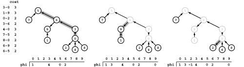
We start at 0, follow the path to the root, set pt[5] to 0, then work down the path, first setting 6 to make pt[6] - pt[5] equal to the cost of 6-5, then setting p[3] to make p[3] - p[6] equal to the cost of 3-6, and so forth (left). Then we start at 1 and follow parent links until hitting a vertex whose potential is known (6 in this case) and work down the path to compute potentials on 9 and 1 (center). When we start at 2, we can compute its potential from its parent (right); when we start at 3, we see that its potential is already known, and so forth. In this example, when we try each vertex after 1, we either find that its potential is already done or we can compute the value from its parent. We never retrace an edge, no matter what the tree structure, so the total running time is linear.

the path to r, but in reverse direction for each edge. Program 22.11 is an implementation of this idea, in the form of a function that augments a cycle and also returns an edge that is emptied or filled by the augmentation.

The implementation in Program 22.11 uses a simple technique to avoid paying the cost of initializing all the marks each time that we call it. We maintain the marks as global variables, initialized to zero. Each time that we seek an LCA, we increment a global counter and mark vertices by setting their corresponding entry in a vertex-indexed vector to that counter. After initialization, this technique allows us to perform the computation in time proportional to the length of the cycle. In typical problems, we might augment along a large number of small cycles, so the time saved can be substantial. As we learn, the same technique is useful in saving time in other parts of the implementation.

Our third tree-manipulation task is to substitute an edge u-v for another edge in the cycle that it creates with tree edges. Program 22.12 is an implementation of a function that accomplishes this task for the parent-link representation. Again, the LCA of u and v is important, because the edge to be removed is either on the path from u to the LCA or on the path from v to the LCA. Removing an edge detaches all its descendants from the tree, but we can repair the damage by reversing the links between u-v and the removed edge, as illustrated in Program 22.48.

These three implementations support the basic operations underlying the network simplex algorithm: We can choose an eligible edge by examining reduced costs and flows; we can use the parent-link representation of the spanning tree to augment along the negative cycle

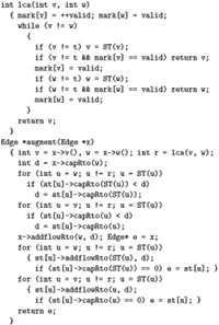
Figure 22.48 Spanning tree substitution

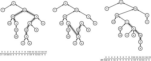
This example illustrates the basic tree-manipulation operation in the network simplex algorithm for the parent-link representation. At left is a sample tree with links all pointing upwards, as indicated by the parent-link structure ST. (In our code, the function ST computes the parent of the given vertex from the edge pointer in the vertex-indexed vector st.) Adding the edge 1-2 creates a cycle with the paths from 1 and 2 to their LCA, 11. If we then delete one of those edges, say 0-3, the structure remains a tree. To update the parent-link array to reflect the change, we switch the directions of all the links from 2 up to 3 (center). The tree at right is the same tree with node positions changed so that links all point up, as indicated by the parent-link array that represents the tree (bottom right).

formed with tree edges and the chosen eligible edge; and we can update the tree and recalculate potentials. These operations are illustrated for an example flow network in Figures 22.49 and 22.50.

Figure 22.49 illustrates initialization of the data structures using a dummy edge with the maxflow on it, as in Figure 22.42. Shown there are an initial feasible spanning tree with its parent-link representation, the corresponding vertex potentials, the reduced costs for the nontree edges, and the initial set of eligible edges. Also, rather than computing the maxflow value in the implementation, we use the outflow from the source, which is guaranteed to be no less than the maxflow value; we use the maxflow value here to make the operation of the algorithm easier to trace.

Figure 22.50 illustrates the changes in the data structures for each of a sequence of eligible edges and augmentations around negative-cost cycles. The sequence does not reflect any particular method for choosing eligible edges; it represents the choices that make the augmenting paths the same as depicted in Program 22.42. These figures show all vertex potentials and all reduced costs after each cycle augmentation, even though many of these numbers are implicitly defined and are not necessarily computed explicitly by typical implementations. The purpose of these two figures is to illustrate the overall progress of the algorithm and the state of the data structures as the algorithm moves

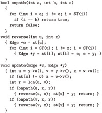
from one feasible spanning tree to another simply by adding an eligible edge and removing a tree edge on the cycle that is formed.

One critical fact that is illustrated in the example in Program 22.50 is that the algorithm might not even terminate, because full or empty edges on the spanning tree can stop us from pushing flow along the negative cycle that we identify. That is, we can identify an eligible edge and the negative cycle that it makes with spanning tree edges, but the maximum amount of flow that we can push along the cycle may be 0. In this case, we still substitute the eligible edge for an edge on the

Figure 22.49 Network simplex initialization

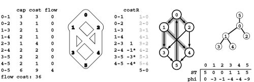
To initialize the data structures for the network simplex algorithm, we start with zero flow on all edges (left), then add a dummy edge 0-5 from source to sink with flow no less than the maxflow value (for clarity, we use a value equal to the maxflow value here). The cost value 9 for the dummy edge is greater than the cost of any cycle in the network; in the implementation, we use the value CV. The dummy edge is not shown in the flow network, but it is included in the residual network (center).

We initialize the spanning tree with the sink at the root, the source as its only child, and a search tree of the graph induced by the remaining nodes in the residual network. The implementation uses the parent-edge representation of the tree in the array st and the related parent-vertex function ST; our figures depict this representation and two others: the rooted representation shown on the right and the set of shaded edges in the residual network.

The vertex potentials are in the pt array and are computed from the tree structure so as to make the difference of a tree edge’s vertex potentials equal to its cost.

The column labeled costR in the center gives the reduced costs for nontree edges, which are computed for each edge by adding the difference of its vertex potentials to its cost. Reduced costs for tree edges are zero and left blank. Empty edges with negative reduced cost and full edges with positive reduced cost (eligible edges) are marked with asterisks.

cycle, but we make no progress in reducing the cost of the flow. To ensure that the algorithm terminates we need to prove that we cannot end up in an endless sequence of zero-flow augmentations.

If there is more than one full or empty edge on the augmenting cycle, the substitution algorithm in Program 22.12 always deletes from the tree the one closest to the LCA of the eligible edge’s two vertices. Fortunately, it has been shown that this particular strategy for choosing the edge to remove from the cycle suffices to ensure that the algorithm terminates (see reference section).

The final important choice that we face in developing an implementation of the network simplex algorithm is a strategy for identifying eligible edges and choosing one to add to the tree. Should we maintain a data structure containing eligible edges? If so, how sophisticated a data structure is appropriate? The answer to these questions depends somewhat on the application and the dynamics of solving particular instances of the problem. If the total number of eligible edges is small, then it is worthwhile to maintain a separate data structure; if most edges are eligible most of the time, it is not. Maintaining a separate data structure could spare us the expense of searching for eligible edges, but also could require costly update computations. What criteria should we use to pick from among the eligible edges? Again, there are many that we might adopt. We consider examples in our implementations, then discuss alternatives. For example, Program 22.13 illustrates a function that finds an eligible edge of minimal reduced cost: No other edge gives a cycle for which augmenting along the cycle would lead to a greater reduction in the total cost.

Program 22.14 is a full implementation of the network simplex algorithm that uses the strategy of choosing the eligible edge giving a negative cycle whose cost is highest in absolute value. The implementation

Figure 22.50 Residual networks and spanning trees (network simplex)

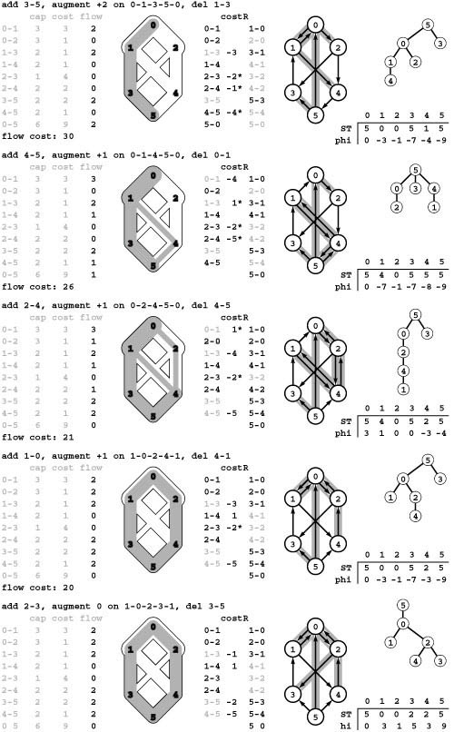
Each row in this figure corresponds to an iteration of the network simplex algorithm following the initialization depicted in Program 22.49: On each iteration, it chooses an eligible edge, augments along a cycle, and updates the data structures as follows: First, the flow is augmented, including implied changes in the residual network. Second, the tree structure ST is changed by adding an eligible edge and deleting an edge on the cycle that it makes with tree edges. Third, the table of potentials phi is updated to reflect the changes in the tree structure. Fourth, the reduced costs of the nontree edges (column marked costR in the center) are updated to reflect the potential changes, and these values used to identify empty edges with negative reduced cost and full edges with positive reduced costs as eligible edges (marked with asterisks on reduced costs). Implementations need not actually make all these computations (they only need to compute potential changes and reduced costs sufficient to identify an eligible edge), but we include all the numbers here to provide a full illustration of the algorithm.

The final augmentation for this example is degenerate. It does not increase the flow, but it leaves no eligible edges, which guarantees that the flow is a mincost maxflow.

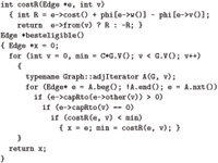
uses the tree-manipulation functions and the eligible-edge search of Programs 22.10 through 22.13, but the comments that we made regarding our first cycle-canceling implementation (Program 22.9) apply: It is remarkable that such a simple piece of code is sufficiently powerful to provide useful solutions in the context of a general problem-solving model with the reach of the mincost-flow problem.

The worst-case performance bound for Program 22.14 is at least a factor of V lower than that for the cycle-canceling implementation in Program 22.9, because the time per iteration is just E (to find the eligible edge) rather than V E (to find a negative cycle). Although we might suspect that using the maximum augmentation will result in fewer augmentations than just taking the first negative cycle provided by the Bellman–Ford algorithm, that suspicion has not been proved valid. Specific bounds on the number of augmenting cycles used are difficult to develop, and, as usual, these bounds are far higher than the numbers that we see in practice. As mentioned earlier, there are

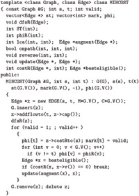
theoretical results demonstrating that certain strategies can guarantee that the number of augmenting cycles is bounded by a polynomial in the number of edges, but practical implementations typically admit an exponential worst case.

In light of these considerations, there are many options to consider in pursuit of improved performance. For example, Program 22.15 is another implementation of the network simplex algorithm. The straightforward implementation in Program 22.14 always takes time proportional to V to revalidate the tree potentials and always takes time proportional to E to find the eligible edge with the largest reduced cost. The implementation in Program 22.15 is designed to eliminate both of these costs in typical networks.

First, even if choosing the maximum edge leads to the fewest number of iterations, expending the effort of examining every edge to find the maximum edge may not be worthwhile. We could do numerous augmentations along short cycles in the time that it takes to scan all the edges. Accordingly, it is worthwhile to consider the strategy of using any eligible edge, rather than taking the time to find a particular one. In the worst case, we might have to examine all the edges or a substantial fraction of them to find an eligible edge, but we typically expect to need to examine relatively few edges to find an eligible one. One approach is to start from the beginning each time; another is to pick a random starting point (see Exercise 22.126). This use of randomness also makes an artificially long sequence of augmenting paths unlikely.

Second, we adopt a lazy approach to computing potentials. Rather than compute all the potentials in the vertex-indexed vector phi, then refer to them when we need them, we call the function phiR to get each potential value; it travels up the tree to find a valid potential, then computes the necessary potentials on that path. To implement this approach, we simply change the function that defines the cost to use the function call phiR(u), instead of the array access phi[u]. In the worst case, we calculate all the potentials in the same way as before; but if we examine only a few eligible edges, then we calculate only those potentials that we need to identify them.

Such changes do not affect the worst-case performance of the algorithm, but they certainly speed it up in practical applications. Several other ideas for improving the performance of the network

simplex algorithm are explored in the exercises (see Exercises 22.126 through 22.130); those represent only a small sample of the ones that have been proposed.

As we have emphasized throughout this book, the task of analyzing and comparing graph algorithms is complex. With the network simplex algorithm, the task is further complicated by the variety of different implementation approaches and the broad array of types of applications that we might encounter (see Section 22.5). Which implementation is best? Should we compare implementations based on the worst-case performance bounds that we can prove? How accurately can we quantify performance differences of various implementations, for specific applications. Should we use multiple implementations, each tailored to specific applications?

Readers are encouraged to gain computational experience with various network simplex implementations and to address some of these questions by running empirical studies of the kind that we have emphasized throughout this book. When seeking to solve mincost flow problems, we are faced with the familiar fundamental challenges, but the experience that we have gained in tackling increasingly difficult problems throughout this book provides ample background to develop efficient implementations that can effectively solve a broad variety of important practical problems. Some such studies are described in the exercises at the end of this and the next section, but these exercises should be viewed as a starting point. Each reader can craft a new empirical study that sheds light on some particular implementation/application pair of interest.

The potential to improve performance dramatically for critical applications through proper deployment of classic data structures and algorithms (or development of new ones) for basic tasks makes the study of network-simplex implementations a fruitful research area, and there is a large literature on network simplex implementations. In the past, progress in this research has been crucial, because it helps reduce the huge cost of solving network simplex problems. People tend to rely on carefully crafted libraries to attack these problems, and that is still appropriate in many situations. However, it is difficult for such libraries to keep up with recent research and to adapt to the variety of problems that arise in new applications. With the speed and size of modern computers, accessible implementations like Programs 22.12 and 22.13 can be starting points for the development of effective problem-solving tools for numerous applications.

Exercises

• 22.116 Give a maxflow with associated feasible spanning tree for the flow network shown in Program 22.10.

• 22.117 Implement the dfsR function for Program 22.14.

• 22.118 Implement a function that removes cycles of partial edges from a given network’s flow and builds a feasible spanning tree for the resulting flow, as illustrated in Program 22.44. Package your function so that it could be used to build the initial tree in Program 22.14 or Program 22.15.

22.119 In the example in Program 22.46, show the effect of reversing the direction of the edge connecting 6 and 5 on the potential tables.

• 22.120 Construct a flow network and exhibit a sequence of augmenting edges such that the generic network simplex algorithm does not terminate.

• 22.121 Show, in the style of Program 22.47, the process of computing potentials for the tree rooted at 0 in Program 22.46.

22.122 Show, in the style of Program 22.50, the process of computing a min-cost maxflow in the flow network shown in Program 22.10, starting with the basic maxflow and associated basic spanning tree that you found in Exercise 22.116.

• 22.123 Suppose that all nontree edges are empty. Write a function that computes the flows in the tree edges, putting the flow in the edge connecting v and its parent in the tree in the vth entry of a vector flow.

• 22.124 Do Exercise 22.123 for the case where some nontree edges may be full.

22.125 Use Program 22.12 as the basis for an MST algorithm. Run empirical tests comparing your implementation with the three basic MST algorithms described in Chapter 20 (see Exercise 20.66).

22.126 Describe how to modify Program 22.15 such that it starts the scan for an eligible edge at a random edge rather than at the beginning each time.

22.127 Modify your solution to Exercise 22.126 such that each time it searches for an eligible edge it starts where it left off in the previous search.

22.128 Modify the private member functions in this section to maintain a triply linked tree structure that includes each node’s parent, leftmost child, and right sibling (see Section 5.4). Your functions to augment along a cycle and substitute an eligible edge for a tree edge should take time proportional to the length of the augmenting cycle, and your function to compute potentials should take time proportional to the size of the smaller of the two subtrees created when the tree edge is deleted.

• 22.129 Modify the private member functions in this section to maintain, in addition to basic parent-edge tree vector, two other vertex-indexed vectors: one containing each vertex’s distance to the root, the other containing each vertex’s successor in a DFS. Your functions to augment along a cycle and substitute an eligible edge for a tree edge should take time proportional to the length of the augmenting cycle, and your function to compute potentials should take time proportional to the size of the smaller of the two subtrees created when the tree edge is deleted.

• 22.130 Explore the idea of maintaining a generalized queue of eligible edges. Consider various generalized-queue implementations and various improvements to avoid excessive edge-cost calculations, such as restricting attention to a subset of the eligible edges so as to limit the size of the queue or possibly allowing some ineligible edges to remain on the queue.

• 22.131 Run empirical studies to determine the number of iterations, the number of vertex potentials calculated, and the ratio of the running time to E for several versions of the network simplex algorithm, for various networks (see Exercises 22.7–12). Consider various algorithms described in the text and in the previous exercises, and concentrate on those that perform the best on huge sparse networks.

• 22.132 Write a client program that does dynamic graphical animations of network simplex algorithms. Your program should produce images like those in Program 22.50 and the other figures in this section (see Exercise 22.48). Test your implementation for the Euclidean networks among Exercises 22.7–12.

Figure 22.51 Reduction from shortest paths

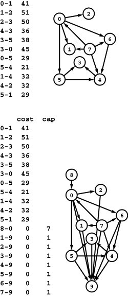
Finding a single-source–shortest-paths tree in the network at the top is equivalent to solving the mincost-maxflow problem in the flow network at the bottom.

22.7 Mincost-Flow Reductions

Mincost flow is a general problem-solving model that can encompass a variety of useful practical problems. In this section, we substantiate this claim by proving specific reductions from a variety of problems to mincost flow.

The mincost-flow problem is obviously more general than the maxflow problem, since any mincost maxflow is an acceptable solution to the maxflow problem. Specifically, if we assign to the dummy edge a cost 1 and to all other edges a cost 0 in the construction of Program 22.42, any mincost maxflow minimizes the flow in the dummy edge and therefore maximizes the flow in the original network. Therefore, all the problems discussed in Section 22.4 that reduce to the maxflow problem also reduce to the mincost-flow problem. This set of problems includes bipartite matching, feasible flow, and mincut, among numerous others.

More interesting, we can examine properties of our algorithms for the mincost-flow problem to develop new generic algorithms for the maxflow problem. We have already noted that the generic cycle-canceling algorithm for the mincost-maxflow problem gives a generic augmenting-path algorithm for the maxflow problem. In particular, this approach leads to an implementation that finds augmenting paths without having to search the network (see Exercises 22.133 and 22.134). On the other hand, the algorithm might produce zero-flow augmenting paths, so its performance characteristics are difficult to evaluate (see reference section).

The mincost-flow problem is also more general than the shortest-paths problem, by the following simple reduction.

Property 22.29 The single-source–shortest-paths problem (in networks with no negative cycles) reduces to the mincost–feasible-flow problem.

Proof: Given a single-source–shortest-paths problem (a network and a source vertex s), build a flow network with the same vertices, edges, and edge costs; and give each edge unlimited capacity. Add a new source vertex with an edge to s that has cost zero and capacity V-1 and a new sink vertex with edges from each of the other vertices with costs zero and capacities 1. This construction is illustrated in Program 22.51.

Solve the mincost–feasible-flow problem on this network. If necessary, remove cycles in the solution to produce a spanning-tree solution. This spanning tree corresponds directly to a shortest-paths spanning tree of the original network. Detailed proof of this fact is left as an exercise (see Exercise 22.138).

Thus, all the problems discussed in Section 21.6 that reduce to the single-source–shortest-paths problem also reduce to the mincost-flow problem. This set of problems includes job scheduling with deadlines and difference constraints, among numerous others.

As we found when studying maxflow problems, it is worthwhile to consider the details of the operation of the network simplex algorithm when solving a shortest-paths problem using the reduction of Property 22.29. In this case, the algorithm maintains a spanning tree rooted at the source, much like the search-based algorithms that we considered in Chapter 21, but the node potentials and reduced costs provide increased flexibility in developing methods to choose the next edge to add to the tree.

We do not generally exploit the fact that the mincost-flow problem is a proper generalization of both the maxflow and the shortest-paths problems, because we have specialized algorithms with better performance guarantees for both problems. If such implementations are not available, however, a good implementation of the network simplex algorithm is likely to produce quick solutions to particular instances of both problems. Of course, we must avoid reduction loops when using or building network-processing systems that take advantage of such reductions. For example, the cycle-canceling implementation in Program 22.9 uses both maxflow and shortest paths to solve the mincost-flow problem (see Exercise 21.96).

Next, we consider equivalent network models. First, we show that assuming that costs are nonnegative is not restrictive, as we can transform networks with negative costs into networks without them.

Property 22.30 In mincost-flow problems, we can assume, without loss of generality, that edge costs are nonnegative.

Proof: We prove this fact for feasible mincost flows in distribution networks. The same result is true for mincost maxflows because of the equivalence of the two problems proved in Property 22.22 (see Exercises 22.143 and 22.144).

Given a distribution network, we replace any edge u-v that has cost x < 0 and capacity c by an edge v-u of the same capacity that has cost −x (a positive number). Furthermore, we can decrement the supply-demand value of u by c and increment the supply-demand value of v by c. This operation corresponds to pushing c units of flow from u to v and adjusting the network accordingly.

For negative-cost edges, if a solution to the mincost-flow problem for the transformed network puts flow f in the edge v-u, we put flow c − f in u-v in the original network; for positive-cost edges, the transformed network has the same flow as in the original. This flow assignment preserves the supply or demand constraint at all the vertices.

The flow in v-u in the transformed network contributes fx to the cost and the flow in u-v in the original network contributes −cx + fx to the cost. The first term in this expression does not depend on the flow, so the cost of any flow in the transformed network is equal to the cost of the corresponding flow in the original network plus the sum of the products of the capacities and costs of all the negative-cost edges (which is a negative quantity). Any minimal-cost flow in the transformed network is therefore a minimal-cost flow in the original network.

This reduction shows that we can restrict attention to positive costs, but we generally do not bother to do so in practice because our implementations in Sections 22.5 and 22.6 work exclusively with residual networks and handle negative costs with no difficulty. It is important to have some lower bound on costs in some contexts, but that bound does not need to be zero (see Exercise 22.145).

Next, we show, as we did for the maxflow problem, that we could, if we wanted, restrict attention to acyclic networks. Moreover, we can also assume that edges are uncapacitated (there is no upper bound on the amount of flow in the edges). Combining these two variations leads to the following classic formulation of the mincost-flow problem.

Transportation Solve the mincost-flow problem for a bipartite distribution network where all edges are directed from a supply vertex to a demand vertex and have unlimited capacity. As discussed at the beginning of this chapter (see Figure 22.2), the usual way to think of this problem is as modeling the distribution of goods from warehouses (supply vertices) to retail outlets (demand vertices) along distribution channels (edges) at a certain cost per unit amount of goods.

Property 22.31 The transportation problem is equivalent to the mincost-flow problem.

Proof: Given a transportation problem, we can solve it by assigning a capacity for each edge higher than the supply or demand values of the vertices that it connects and solving the resulting mincost–feasible-flow problem on the resulting distribution network. Therefore, we need only to establish a reduction from the standard problem to the transportation problem.

For variety, we describe a new transformation, which is linear only for sparse networks. A construction similar to the one that we used in the proof of Property 22.16 establishes the result for nonsparse networks (see Exercise 22.148).

Given a standard distribution network with V vertices and E edges, build a transportation network with V supply vertices, E demand vertices and 2E edges, as follows. For each vertex in the original network, include a vertex in the bipartite network with supply or demand value set to the original value plus the sum of the capacities of the outgoing edges; and for each edge u-v in the original network with capacity c, include a vertex in the bipartite network with supply or demand value -c (we use the notation [u-v] to refer to this vertex). For each edge u-v in the original network, include two edges in the bipartite network: one from u to [u-v] with the same cost, and one from v to [u-v] with cost 0.

The following one-to-one correspondence preserves costs between flows in the two networks: An edge u-v has flow value f in the original network if and only if edge u-[u-v] has flow value f, and edge v-[u-v] has flow value c-f in the bipartite network (those two flows must sum to c because of the supply–demand constraint at vertex [u-v]. Thus, any mincost flow in one network corresponds to a mincost flow in the other.

Since we have not considered direct algorithms for solving the transportation problem, this reduction is of academic interest only. To use it, we would have to convert the resulting problem back to a (different) mincost-flow problem, using the simple reduction mentioned at the beginning of the proof of Property 22.31. Perhaps such networks admit more efficient solutions in practice; perhaps they do not. The point of studying the equivalence between the transportation problem and the mincost-flow problem is to understand that removing capacities and restricting attention to bipartite networks would seem to simplify the mincost-flow problem substantially; however, that is not the case.

We need to consider another classical problem in this context. It generalizes the bipartite-matching problem that is discussed in detail in Section 22.4. Like that problem, it is deceptively simple.

Assignment Given a weighted bipartite graph, find a set of edges of minimum total weight such that each vertex is connected to exactly one other vertex.

For example, we might generalize our job-placement problem to include a way for each company to quantify its desire for each applicant (say by assigning an integer to each applicant, with lower integers going to the better applicants) and for each applicant to quantify his or her desire for each company. Then, a solution to the assignment problem would provide a reasonable way to take these relative preferences into account.

Property 22.32 The assignment problem reduces to the mincost-flow problem.

Proof: This result can be established via a simple reduction to the transportation problem. Given an assignment problem, construct a transportation problem with the same vertices and edges, with all vertices in one of the sets designated as supply vertices with value 1 and all vertices in the other set designated as demand vertices with value 1. Assign capacity 1 to each edge, and assign a cost corresponding to that edge’s weight in the assignment problem. Any solution to this instance of the transportation problem is simply a set of edges of minimal total cost that each connect a supply vertex to a demand vertex and therefore corresponds directly to a solution to the original assignment problem.

Reducing this instance of the transportation problem to the mincost-maxflow problem gives a construction that is essentially equivalent to the construction that we used to reduce the bipartite-matching problem to the maxflow problem (see Exercise 22.158).

This relationship is not known to be an equivalence. There is no known way to reduce a general mincost-flow problem to the assignment problem. Indeed, like the single-source–shortest-paths problem and the maxflow problem, the assignment problem seems to be easier than the mincost-flow problem in the sense that algorithms that solve it are known that have better asymptotic performance than the best known algorithms for the mincost-flow problem. Still, the network simplex algorithm is sufficiently well refined that a good implementation of it is a reasonable choice for solving assignment problems. Moreover, as with maxflow and shortest paths, we can tailor the network simplex algorithm to get improved performance for the assignment problem (see reference section).

Our next reduction to the mincost-flow problem brings us back to a basic problem related to paths in graphs like the ones that we first considered in Section 17.7. As in the Euler-path problem, we want a path that includes all the edges in a graph. Recognizing that not all graphs have such a path, we relax the restriction that edges must appear only once.

Mail carrier Given a network (weighted digraph), find a cyclic path of minimal weight that includes each edge at least once (see Figure 22.52). Recall that our basic definitions in Chapter 17 make the distinction between cyclic paths (which may revisit vertices and edges) and cycles (which consist of distinct vertices, except the first and the final, which are the same).

The solution to this problem would describe the best route for a mail carrier (who has to cover all the streets on her route) to follow. A solution to this problem might also describe the route that a snow-plow should take during a snowstorm, and there are many similar applications.

The mail carrier’s problem is an extension of the Euler-tour problem that we discussed in Section 17.7: The solution to Exercise 17.92 is a simple test for whether a digraph has an Euler tour, and Program 17.14 is an effective way to find an Euler tour for such digraphs. That tour solves the mail carrier’s problem because it includes each edge exactly once—no path could have lower weight. The problem becomes more difficult when indegrees and outdegrees are not necessarily

Figure 22.52 Mail carrier’s problem

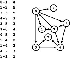
Finding the shortest path that includes each edge at least once is a challenge even for this small network, but the problem can be solved efficiently through reduction to the mincost-flow problem.

equal. In the general case, some edges must be traversed more than once: The problem is to minimize the total weight of all the multiply traversed edges.

Property 22.33 The mail carrier’s problem reduces to the mincost-flow problem.

Proof: Given an instance of the mail carrier’s problem (a weighted digraph), define a distribution network on the same vertices and edges, with all the vertex supply or demand values set to 0, edge costs set to the weights of the corresponding edge, and no upper bounds on edge capacities, but all edge capacities constrained to be greater than 1. We interpret a flow value f in an edge u-v as saying that the mail carrier needs to traverse u-v a total of f times.

Find a mincost flow for this network by using the transformation of Exercise 22.146 to remove the lower bound on edge capacities. The flow-decomposition theorem says that we can express the flow as a set of cycles, so we can build a cyclic path from this flow in the same way that we built an Euler tour in an Eulerian graph: We traverse any cycle, taking a detour to traverse another cycle whenever we encounter a node that is on another cycle.

A careful look at the mail carrier’s problem illustrates yet again the fine line between trivial and intractable in graph algorithms. Suppose that we consider the two-way version of the problem where the network is undirected, and the mail carrier must travel in both directions along each edge. Then, as we noted in Section 18.5, depth-first search (or any graph search) will provide an immediate solution. If, however, it suffices to traverse each undirected edge in either direction, then a solution is significantly more difficult to formulate than is the simple reduction to mincost flow that we just examined, but the problem is still tractable. If some edges are directed and others undirected, the problem becomes NP-hard (see reference section).

These are only a few of the scores of practical problems that have been formulated as mincost-flow problems. The mincost-flow problem is even more versatile than the maxflow problem or shortest-paths problems, and the network simplex algorithm effectively solves all problems encompassed by the model.

As we did when we studied maxflow, we can examine how any mincost-flow problem can be cast as an LP problem, as illustrated in

Figure 22.53 LP formulation of a mincostmaxflow problem

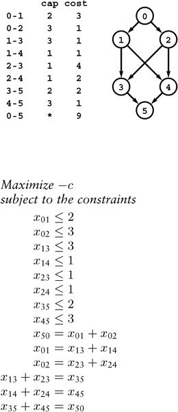
This linear program is equivalent to the mincost-maxflow problem for the sample network of Program 22.40. The edge equalities and vertex inequalities are the same as in Program 22.39, but the objective is different. The variable c represents the total cost, which is a linear combination of the other variables. In this case, c =− 9x₅₀ +3x₀₁ + x ₀₂ + x ₁₃ + x₁₄ +4x₂₃ +2x₂₄ +2x₃₅ + x ₄₅.

Figure 22.53. The formulation is a straightforward extension of the maxflow formulation: We add equations that set a dummy variable to be equal to the cost of the flow, then set the objective so as to minimize that variable. LP models allow addition of arbitrary (linear) constraints. Some constraints may lead to problems that still may be equivalent to mincost-flow problems, but others do not. That is, many problems do not reduce to mincost-flow problems: In particular, LP encompasses a much broader set of problems. The mincost-flow problem is a next step toward that general problem-solving model, which we consider in Part 8.

There are other models that are even more general than the LP model; but LP has the additional virtue that, while LP problems are in general more difficult than mincost-flow problems, effective and efficient algorithms have been invented to solve them. Indeed, perhaps the most important such algorithm is known as the simplex method: The network simplex method is a specialized version of the simplex method that applies to the subset of LP problems that correspond to mincost-flow problems, and understanding the network simplex algorithm is a helpful first step in understanding the simplex algorithm.