
Chapter 7: Performance Optimization
Amazon Redshift provides out-of-the-box capabilities for most workloads. Amazon Redshift defaults the table design choices, such as sort and distribution key, to AUTO and can learn from the query workloads to automatically set up the right structure. For more information, see Working with automatic table optimization (https://docs.aws.amazon.com/redshift/latest/dg/t_Creating_tables.html).
As a user of Amazon Redshift, it provides the necessary levers so that you can further optimize/pick a different choice when needed. The sort, distribution key, and table encoding choices have influential effects on the performance of queries, and in this chapter, we will discuss the optimization techniques we can use to improve these throughputs. Also, we will take a deep dive into analyzing queries to understand the rationale behind the tuning exercise.
In this chapter, we will cover the following recipes:
- Amazon Redshift Advisor
- Managing column compression
- Managing data distribution
- Managing sort keys
- Analyzing and improving queries
- Configuring workload management (WLM)
- Utilizing Concurrency Scaling
- Optimizing Spectrum queries
Technical requirements
You will need the following technical requirements to complete the recipes in this chapter:
- Access to the AWS Console.
- The AWS administrator should create an IAM user by following Recipe 1 – Creating an IAM User, in the Appendix. This IAM user will be used in some of the recipes in this chapter.
- The AWS administrator should create an IAM role by following Recipe 3: Creating IAM Role for an AWS service, in the Appendix. This IAM role will be used in some of the recipes in this chapter.
- The AWS administrator should deploy the AWS CloudFormation template (https://github.com/PacktPublishing/Amazon-Redshift-Cookbook/blob/master/Chapter07/chapter_7_CFN.yaml) and create two IAM policies:
a. An IAM policy that's attached to the IAM user, which will give them access to Amazon Redshift, Amazon EC2, AWS Secrets Manager, AWS IAM, AWS CloudFormation, AWS KMS, AWS Glue, and Amazon S3.
b. An IAM policy that's attached to the IAM role, which will allow the Amazon Redshift cluster to access Amazon S3.
- Attach the IAM role to the Amazon Redshift cluster by following Recipe 4 – Attaching an IAM Role to the Amazon Redshift cluster, in the Appendix. Take note of the IAM's role name. We will reference it in this chapter's recipes as [Your-Redshift_Role].
- An Amazon Redshift cluster deployed in AWS region eu-west-1.
- Amazon Redshift cluster master user credentials.
- Access to any SQL interface, such as a SQL client or the Amazon Redshift Query Editor.
- An AWS account number. We will reference it in this chapter's recipes as [Your-AWS_Account_Id].
- This chapter's code files, which can be found in this book's GitHub repository: https://github.com/PacktPublishing/Amazon-Redshift-Cookbook/tree/master/Chapter07.
Amazon Redshift Advisor
Amazon Redshift Advisor was launched in mid 2018. It runs daily and continuously observes the workload's operational statistics on the cluster with its lens of best practices. Amazon Redshift Advisor uses sophisticated algorithms to provide tailored best practice recommendations, which allows us to get the best possible performance and cost savings. The recommendations are provided which is ranked by order of impact. Amazon Redshift Advisor eases administration. Some of the recommendations include the following:
- Optimization for the COPY command for optimal data ingestion
- Optimization for physical table design
- Optimization for manual workload management
- Cost optimization with a recommendation to delete a cluster after taking a snapshot, if the cluster is not being utilized
Along with the Advisor recommendation, the Automatic Table Optimization feature allows you to apply these recommendations via an auto-requiring administrator intervention, thereby creating a fully self-tuning system.
In this recipe, you will learn where to find Amazon Redshift Advisor so that you can view these recommendations.
Getting ready
To complete this recipe, you will need the following:
- An IAM user with access to Amazon Redshift
- An Amazon Redshift cluster deployed in AWS region eu-west-1
How to do it…
In this recipe, we will use the Amazon Redshift console to access the Advisor recommendation for your cluster. Let's get started:
- Navigate to the AWS Management Console and select Amazon Redshift.
- On the left-hand side, you will see ADVISOR. Click on it:
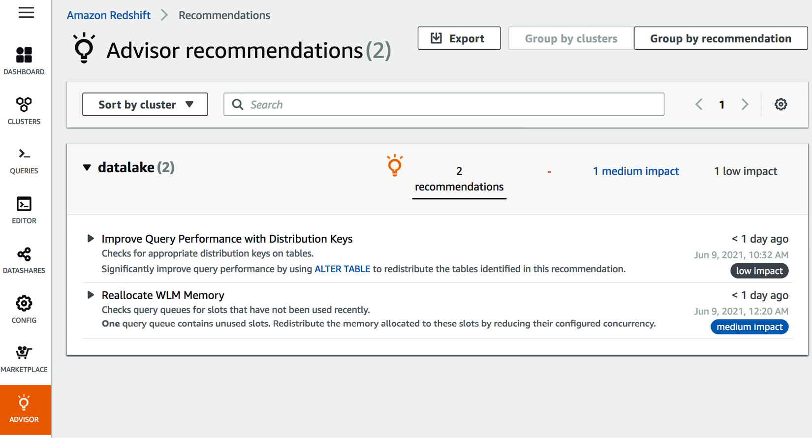
Figure 7.1 – Accessing the Advisor from the AWS Redshift console
- If you have multiple clusters in a region, you can view the recommendations for all the clusters. You can group the recommendations by cluster or by category – cost, performance, security, or other:
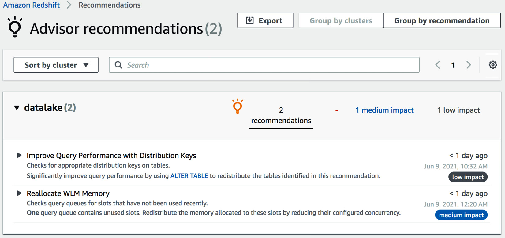
Figure 7.2 – Accessing Amazon Redshift Advisor
- You can distribute the recommendations by exporting the recommendations from the console to a file. To export the recommendations from the Advisor page, select Export:

Figure 7.3 – Amazon Redshift Advisor recommendations
How it works…
Amazon Redshift builds recommendations by continuously analyzing the operational data of your cluster. The Advisor provides recommendations that have a significant impact on the performance of your cluster. The Advisor, alongside the Automatic Table Optimization feature, collects the query access patterns and analyzes them using a machine learning service to predict recommendations about the sort and distribution keys. These recommendations are then applied automatically to the target tables in the cluster. Advisor and Automatic Table Optimization execute during low workload intensity so that user queries are affected.
Managing column compression
Amazon Redshift's columnar architecture stores data columns upon columns on disk. Analytical queries select a subset of the columns and perform aggregation on millions to billions of records. The columnar architecture reduces the I/O by selecting a subset of the columns, thus improving query performance. When data is ingested into the Amazon Redshift table, it provides three to four times compression. This further reduces the storage footprint, which, in turn, reduces I/O and hence improves query performance. Reducing the storage footprint also saves you money. Amazon Redshift Advisor provides recommendations for compressing any uncompressed tables.
In this recipe, you will learn how Amazon Redshift automatically applies compression to new and existing tables. You will also learn how column-level compression can be modified for existing columns.
Getting ready
To complete this recipe, you will need the following:
- An IAM user with access to Amazon Redshift.
- An Amazon Redshift cluster deployed in AWS region eu-west-1.
- Amazon Redshift cluster master user credentials.
- Access to any SQL interface, such as a SQL client or the Amazon Redshift Query Editor.
- An IAM role attached to an Amazon Redshift cluster that can access Amazon S3. We will reference it in this recipe as [Your-Redshift_Role].
- An AWS account number. We will reference it in this recipe as [Your-AWS_Account_Id].
How to do it…
In this recipe, we will be analyzing the table-level compression that's applied by Amazon Redshift automatically. Let's get started:
- Connect to the Amazon Redshift cluster using a SQL client or the Query Editor. Then, create the customer table using the following command:
drop table if exists customer;
CREATE TABLE customer
(
C_CUSTKEY BIGINT NOT NULL,
C_NAME VARCHAR(25),
C_ADDRESS VARCHAR(40),
C_NATIONKEY BIGINT,
C_PHONE VARCHAR(15),
C_ACCTBAL DECIMAL(18,4),
C_MKTSEGMENT VARCHAR(10),
C_COMMENT VARCHAR(117)
)
diststyle AUTO;
- Now, let's analyze the compression types that have been applied to the columns. Execute the following command:
SELECT "column", type, encoding FROM pg_table_def
WHERE tablename = 'customer';
Here is the expected output:
column | type | encoding
--------------+------------------------+----------
c_custkey | bigint | az64
c_name | character varying(25) | lzo
c_address | character varying(40) | lzo
c_nationkey | bigint | az64
c_phone | character varying(15) | lzo
c_acctbal | numeric(18,4) | az64
c_mktsegment | character varying(10) | lzo
c_comment | character varying(117) | lzo
Amazon Redshift automatically applies a compression type of az64 for AZ64 for the INT, SMALLINT, BIGINT, TIMESTAMP, TIMESTAMPTZ, DATE, and NUMERIC column types. Az64 is Amazon's proprietary compression encoding algorithm, and it's designed to achieve a high compression ratio and improved query processing. The default encoding of lzo is applied to the varchar and character columns.
Reference to Different Encoding Types in Amazon Redshift
https://docs.aws.amazon.com/redshift/latest/dg/c_Compression_encodings.html
- Now, let's recreate the customer table by encoding C_CUSTKEY as raw using the following SQL:
drop table if exists customer ;
CREATE TABLE customer
(
C_CUSTKEY BIGINT NOT NULL encode raw,
C_NAME VARCHAR(25),
C_ADDRESS VARCHAR(40),
C_NATIONKEY BIGINT,
C_PHONE VARCHAR(15),
C_ACCTBAL DECIMAL(18,4),
C_MKTSEGMENT VARCHAR(10),
C_COMMENT VARCHAR(117)
)
diststyle AUTO;
SELECT "column", type, encoding FROM pg_table_def
WHERE tablename = 'customer';
Here is the expected output:
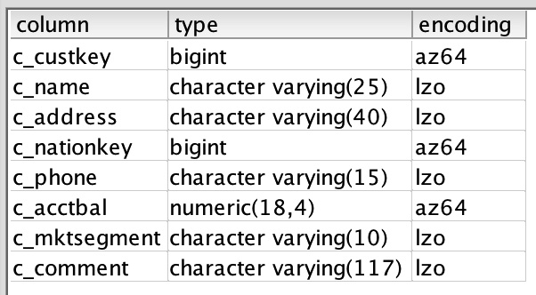
Figure 7.4 – Output of the preceding query
Notice that the c_custkey column has been encoded with a raw encoding (none).
- Now, let's use COPY to load data from Amazon S3 using the following command, replacing [Your-AWS_Account_Id] and [Your-Redshift_Role] with their respective values:
COPY customer from 's3://packt-redshift-cookbook/RetailSampleData/customer/' iam_role 'arn:aws:iam::[Your-AWS_Account_Id]:role/[Your-Redshift_Role]' CSV gzip COMPUPDATE PRESET;
SELECT "column", type, encoding FROM pg_table_def
WHERE tablename = 'customer';
Here is the expected output:
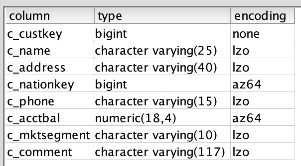
Figure 7.5 – Output of the preceding query
Note
Amazon Redshift command with compupdate on determines the encoding for the columns for an empty table, even for columns set to raw; that is, no compression. Create the table with the c_custkey column set to encode raw. Then, run the COPY command with the compupdate preset option, which determines how the columns for empty tables are encoded. Then, we must verify the encodings of the columns and that the c_custkey column has an encoding type of az64.
How it works…
Amazon Redshift, by default, applies compression, which helps reduce the storage footprint and hence query performance due to a decrease in I/O. Each column can have different encoding types and columns that can grow and shrink independently. For an existing table, you can use the ANALYZE COMPRESSION command to determine the encoding type that results in storage savings. It is a built-in command that will find the optimal compression for each column. You can then apply the recommended compression to the table using the alter statement or by creating a new table with the new encoding types. Then, you can copy the data from the old table to the new table.
Managing data distribution
Distribution style is a table property that dictates how that table's data is distributed throughout the compute nodes. The goal of data distribution is to leverage the massively parallel processing of Amazon Redshift and reduce the I/O during query processing to improve performance. Amazon Redshift Advisor provides actionable recommendations on distribution style for the table via the alter statement. Using automatic table optimization allows you to self-manage the table distribution style based on workload patterns:
- KEY: The value is hashed. The same value goes to the same location (slice).
- ALL: The entirety of the table data goes to the first slice of every compute node.
- EVEN: Round robin data distribution is performed across the compute nodes and slices.
- AUTO: Combines the EVEN, ALL, and KEY distributions:
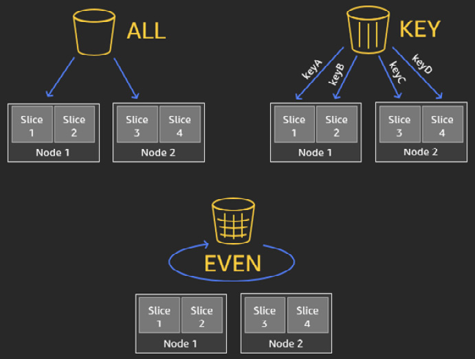
Figure 7.6 – Data distribution styles
In this recipe, you will learn how Amazon Redshift's automatic table style works and the benefits of different distribution styles.
Getting ready
To complete this recipe, you will need the following:
- An IAM user with access to Amazon Redshift.
- An Amazon Redshift cluster deployed in AWS region eu-west-1.
- Amazon Redshift cluster master user credentials.
- Access to any SQL interface, such as a SQL client or the Amazon Redshift Query Editor.
- An IAM role attached to an Amazon Redshift cluster that can access Amazon S3. We will reference it in this recipe as [Your-Redshift_Role].
- An AWS account number. We will reference it in this recipe as [Your-AWS_Account_Id].
How to do it…
In this recipe, we will create a customer table with different distribution keys and analyze their join effectiveness and data distribution:
- Connect to the Amazon Redshift cluster using a SQL client or the Query Editor.
- Create the dwdate table with the default auto-distribution style. Then, run the copy command, replacing [Your-AWS_Account_Id] and [Your-Redshift_Role] with the respective values:
DROP TABLE IF EXISTS dwdate;
CREATE TABLE dwdate
(
d_datekey INTEGER NOT NULL,
d_date VARCHAR(19) NOT NULL,
d_dayofweek VARCHAR(10) NOT NULL,
d_month VARCHAR(10) NOT NULL,
d_year INTEGER NOT NULL,
d_yearmonthnum INTEGER NOT NULL,
d_yearmonth VARCHAR(8) NOT NULL,
d_daynuminweek INTEGER NOT NULL,
d_daynuminmonth INTEGER NOT NULL,
d_daynuminyear INTEGER NOT NULL,
d_monthnuminyear INTEGER NOT NULL,
d_weeknuminyear INTEGER NOT NULL,
d_sellingseason VARCHAR(13) NOT NULL,
d_lastdayinweekfl VARCHAR(1) NOT NULL,
d_lastdayinmonthfl VARCHAR(1) NOT NULL,
d_holidayfl VARCHAR(1) NOT NULL,
d_weekdayfl VARCHAR(1) NOT NULL
);
COPY public.dwdate from 's3://packt-redshift-cookbook/dwdate/' iam_role 'arn:aws:iam::[Your-AWS_Account_Id]:role/[Your-Redshift_Role]' CSV gzip COMPUPDATE PRESET dateformat 'auto';
To verify the distribution style of the dwdate table, execute the preceding command.
Here is the expected output:

Figure 7.7 – Output of the preceding query
Amazon Redshift, by default, sets the distribution style to AUTO(ALL). Amazon Redshift automatically manages the distribution style for the table, and for small tables, it creates a distribution style of ALL. With the ALL distribution style, the data for this table is stored on every compute node slice as 0. The distribution style of ALL is well-suited for small dimension tables, which enables join performance optimization for large tables with smaller dimension tables.
Let's create the customer table with the default auto-distribution style using the following code, replacing [Your-AWS_Account_Id] and [Your-Redshift_Role].
- Now, let's modify the distribution style of the customer table using the c_nationkey column by executing the following query:
alter table customer alter distkey C_NATIONKEY;
- Now, let's verify the distribution style of the customer table by executing the following query:
select "schema", "table", "diststyle", skew_rows
from svv_table_info
where "table" = 'customer';
Here is the expected output:
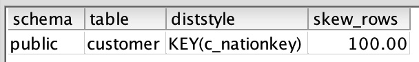
Figure 7.8 – Output of the preceding query
c_nationkey causes the skewness in the distribution, as shown by the skew_row column, since it has less distinct values (low cardinality). Ideally, skew_row should be less than 5. When data is skewed, some compute nodes will do more work compared to others. The performance of the query is affected by the compute node that contains more data.
- Now, let's alter the distribution key for the customer table using the high cardinality column; that is, c_custkey. Execute the following query and verify the table skew:
alter table customer alter distkey c_custkey;
select "schema", "table", "diststyle", skew_rows
from svv_table_info
where "table" = 'customer';
---output----
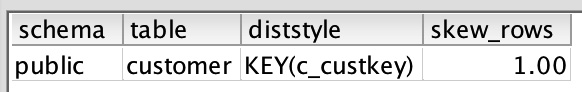
Now, the customer table has low skew_rows, which will ensure all the compute nodes can perform equal work when processing the query.
How it works…
Amazon Redshift data distribution is a physical table property. It determines how the data is distributed across the compute nodes. The purpose of data distribution is to have every compute node work in parallel to execute the workload and reduce the I/O during join performance, to optimize performance. Amazon Redshift's automatic table optimizations enable you to achieve this. You also have the option to select your distribution style to fine-tune your most demanding workloads to achieve significant performance. Creating a Redshift table with auto-table optimization will automatically change the distribution style based on your workload pattern. You can review the alter table recommendations in the svv_alter_table_recommendations view, and the actions that have been applied by automatic table optimization in the svl_auto_worker_action view.
Managing sort keys
Data sorting in Amazon Redshift is a concept regarding how data is physically sorted on the disk. Data sorting is determined by the sortkey property defined in the table. Amazon Redshift automatically creates in-memory metadata called zone maps. Zone maps contain the minimum and maximum values for each block. Zone maps automatically enable you to eliminate I/O from scanning blocks that do not contain data for queries. Sort keys make zone maps more efficient.
sortkey can be defined on one or more columns. The columns that are defined in the sort keys are based on your query pattern. Most frequently, filtered columns are good candidates for the sort key. The sort key column's order is defined from low to high cardinality. Sort keys enable range-restricted scans to prune blocks, eliminating I/O and hence optimizing query performance. Redshift Advisor provides recommendations on optimal sort keys, and automatic table optimization handles the sort key changes based on our query pattern.
In this recipe, you will learn how Amazon Redshift compound sort keys work.
Getting ready
To complete this recipe, you will need the following:
- An IAM user with access to Amazon Redshift.
- An Amazon Redshift cluster deployed in AWS region eu-west-1.
- Amazon Redshift cluster master user credentials.
- Access to any SQL interface, such as a SQL client or the Amazon Redshift Query Editor.
- An IAM role attached to an Amazon Redshift cluster that can access Amazon S3. We will reference it in this recipe as [Your-Redshift_Role].
- An AWS account number. We will reference it in this recipe as [Your-AWS_Account_Id].
How to do it…
In this recipe, we will use the lineitem table with sort keys and analyze the performance queries. Let's get started:
- Connect to the Amazon Redshift cluster using a SQL client or the Query Editor.
- Let's create the lineitem table with the default auto sortkey using the following code. Remember to replace [Your-AWS_Account_Id] and [Your-Redshift_Role] with their respective values:
drop table if exists lineitem;
CREATE TABLE lineitem
(
L_ORDERKEY BIGINT NOT NULL,
L_PARTKEY BIGINT,
L_SUPPKEY BIGINT,
L_LINENUMBER INTEGER NOT NULL,
L_QUANTITY DECIMAL(18,4),
L_EXTENDEDPRICE DECIMAL(18,4),
L_DISCOUNT DECIMAL(18,4),
L_TAX DECIMAL(18,4),
L_RETURNFLAG VARCHAR(1),
L_LINESTATUS VARCHAR(1),
L_SHIPDATE DATE,
L_COMMITDATE DATE,
L_RECEIPTDATE DATE,
L_SHIPINSTRUCT VARCHAR(25),
L_SHIPMODE VARCHAR(10),
L_COMMENT VARCHAR(44)
)
distkey (L_ORDERKEY) ;
COPY lineitem from 's3://packt-redshift-cookbook/lineitem/' iam_role 'arn:aws:iam::[Your-AWS_Account_Id]:role/[Your- Redshift_Role]' CSV gzip COMPUPDATE PRESET;
Note
Depending on the size of the cluster, the COPY command will take around 15 minutes to complete due to the size of the data.
- Let's verify the sort key of the lineitem table with the default auto sortkey using the following query:
select "schema", "table", "diststyle", skew_rows, sortkey1, unsorted
from svv_table_info
where "table" = 'lineitem';
Here is the expected output:
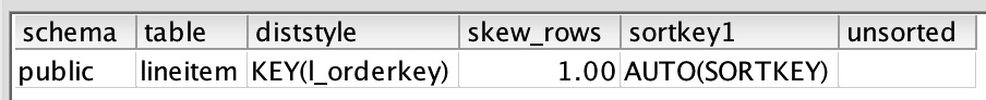
Figure 7.9 – Output of the preceding query
As shown in the preceding output, the lineitem table has been set with AUTO(sortkey). Amazon Redshift Advisor, based on your workload pattern, will make recommendations and the automatic table optimization will alter the table with an optimal sort key.
- To see the effectiveness of block pruning using the sort key, execute the following query and take note of query_id:
SELECT
l_returnflag,
l_linestatus,
sum(l_quantity) as sum_qty,
sum(l_extendedprice) as sum_base_price,
sum(l_extendedprice * (1 - l_discount)) as sum_disc_price,
count(*) as count_order
FROM
lineitem
WHERE
l_shipdate = '1992-01-10'
GROUP BY
l_returnflag,
l_linestatus
ORDER BY
l_returnflag,
l_linestatus;
select PG_LAST_QUERY_ID() as query_id;
Here is the expected output:
query_id
1240454
Note
Amazon Redshift captures the operational statistics of each query step in system tables. Details about Svl_query_summary can be found at https://docs.aws.amazon.com/redshift/latest/dg/r_SVL_QUERY_SUMMARY.html.
- Execute the following query to measure the effectiveness of the sort key for the preceding query, replacing [query_id] with the output from the preceding step:
SELECT query, step, label, is_rrscan, rows, rows_pre_filter, is_diskbased
from svl_query_summary where query in ([query_id])
and label like '%lineitem%'
order by query,step;
Here is the expected output:

rows_pre_filter indicates that Amazon Redshift was effectively able to use the sort key to rows_pre_filtered 4,066,288 down to 18,385. is_rrscan is true for these range scans. Amazon Redshift automatically leverages zone maps to prune out the blocks that do not match the filter criteria of the query.
- Let's alter the lineitem table and add the l_shipdate column as our sortkey. Most of the queries we will run will use l_shipdate as the filter. L_shipdate is a low cardinality column:
alter table lineitem alter sortkey (L_SHIPDATE);
Note
Depending on the size of the cluster, the ALTER statement will take at around 15 minutes to complete due to the size of the data.
To see the effectiveness of sortkey, execute the following query and capture the query ID:
query_id_1
Here is the expected output:
1240216
- Now, let's modify the query so that it purposely casts the l_shipdate column as a varchar data type and then applies the filter. Execute the following modified query and capture the output of query_id:
set enable_result_cache_for_session = off;
SELECT
l_returnflag,
l_linestatus,
sum(l_quantity) as sum_qty,
sum(l_extendedprice) as sum_base_price,
sum(l_extendedprice * (1 - l_discount)) as sum_disc_price,
count(*) as count_order
FROM
lineitem
WHERE
cast(l_shipdate as varchar(10) ) = '1992-01-10'
GROUP BY
l_returnflag,
l_linestatus
ORDER BY
l_returnflag,
l_linestatus;
select PG_LAST_QUERY_ID() as query_id_2;
---expected sample output--—
query_id_2
1240218
- Now, let's execute the following query to analyze the effectiveness of the sort key columns, replacing [query_id_1] and [query_id_2] shown in the preceding steps:
SELECT query, step, label, is_rrscan, rows, rows_pre_filter, is_diskbased
from svl_query_summary where query in ([query_id_1],[ query_id_2])
and label like '%lineitem%'
order by query,step;
Here is the expected output:

Figure 7.10 – Output of the preceding query
[query_id_1], which used l_shipdate to filter rows_pre_filter, is 4066288 versus [query_id_2], which was cast to rows_pre_filter and is 599037902. This means that a full table scan was performed. As a best practice, to make your sort keys effective, avoid applying functions or casting to sort key columns.
How it works…
Using sort keys when creating a table allows you to perform efficient range-restricted scans of the data, when the sort key is referenced in the where conditions. Amazon Redshift automatically leverages the in-memory metadata to prune out the blocks. The sort keys make the zone maps more pristine. Applying sort keys to the most commonly used columns as filters in a query can significantly reduce the I/O, and hence optimize query performance for any workload. You can learn more about sort keys at https://docs.aws.amazon.com/redshift/latest/dg/t_Sorting_data.html.
Analyzing and improving queries
Amazon Redshift defaults the table sort key and distribution key to AUTO. Amazon Redshift can learn from the workloads and automatically set the right sort and distribution style, the two big levers that dictate the table's design and optimization. Amazon Redshift also provides insights into the query plan, which helps optimize the queries when authoring them. This plan contains detailed steps about how to fetch the data.
Getting ready
To complete this recipe, you will need the following:
- An IAM user with access to Amazon Redshift.
- An Amazon Redshift cluster deployed in AWS region eu-west-1.
- Amazon Redshift cluster master user credentials.
- Access to any SQL interface, such as a SQL client or the Amazon Redshift Query Editor.
- An IAM role attached to an Amazon Redshift cluster that can access Amazon S3. We will reference it in this recipe as [Your-Redshift_Role].
- An AWS account number. We will reference it in this recipe as [Your-AWS_Account_Id].
How to do it…
In the recipe, we will use the Retail System Dataset from Chapter 3, Loading and Unloading Data, to perform analytical queries and optimize them:
- Connect to the Amazon Redshift cluster using any SQL interface, such as a SQL client or the Query Editor, and execute EXPLAIN on a query:
explain
SELECT o_orderstatus,
COUNT(o_orderkey) AS orders_count,
SUM(l_quantity) AS quantity,
MAX(l_extendedprice) AS extendedprice
FROM lineitem
JOIN orders ON l_orderkey = o_orderkey
WHERE
L_SHIPDATE = '1992-01-29'
GROUP BY o_orderstatus;
Here is the expected output:
QUERY PLAN
----------------------------------------------------------------------
XN HashAggregate (cost=97529596065.20..97529596065.22 rows=3 width=36)
-> XN Hash Join DS_BCAST_INNER (cost=3657.20..97529594861.20 rows=120400 width=36)
Hash Cond: ("outer".o_orderkey = "inner".l_orderkey)
-> XN Seq Scan on orders (cost=0.00..760000.00 rows=76000000 width=13)
-> XN Hash (cost=3047.67..3047.67 rows=243814 width=31)
-> XN Seq Scan on lineitem (cost=0.00..3047.67 rows=243814 width=31)
Filter: (l_shipdate = '1992-01-29'::date)
As shown in the preceding output, the explain command provides insights into the steps that were performed by the query. As we can see, lineitem and the orders table have been joined using a hash join. Each step also provides the relative cost of comparing the expensive steps in the query for optimization purposes.
Note
Please also see https://docs.aws.amazon.com/redshift/latest/dg/c-query-planning.html for a step-by-step illustration of the query planning and execution steps.
- Now, execute the analytical query using the following command to capture query_id for analysis:
SELECT o_orderstatus,
COUNT(o_orderkey) AS orders_count,
SUM(l_quantity) AS quantity,
MAX(l_extendedprice) AS extendedprice
FROM lineitem
JOIN orders ON l_orderkey = o_orderkey
WHERE L_SHIPDATE = '1992-01-29'
GROUP BY o_orderstatus;
select
PG_LAST_QUERY_ID() as query_id;
Here is the expected output:
query_id
24580051
Note that this query_id that will be used later to analyze the query.
- Execute the following command to analyze the effectiveness of the sort key column on the lineitem table by replacing [query_id] from the preceding step:
SELECT step, label, is_rrscan, rows, rows_pre_filter, is_diskbased
from svl_query_summary where query = [query_id]
order by step;
Here is the expected output:
step | label | is_rrscan | rows | rows_pre_filter | is_diskbased
------+-------------------------------------------+-----------+--------+-----------------+-------------
0 | scan tbl=1450056 name=lineitem | t | 57856 | 599037902 | f
0 | scan tbl=361382 name=Internal Worktable | f | 1 | 0 | f
0 | scan tbl=1449979 name=orders | t | 79119 | 76000000 | f
0 | scan tbl=361380 name=Internal Worktable | f | 173568 | 0 | f
0 | scan tbl=361381 name=Internal Worktable | f | 32 | 0 | f
As we can see, the query optimizer can effectively make use of the range restricted scan (is_rrscan) on the l_shipdate column in the lineitem table, to filter out the rows from 599037902 rows to 57856. This can be compared to the rows_pre_filter and rows columns in the preceding output. Also, none of the steps spill to disk, as indicated by is_diskbased = f.
- Now, let's execute the following command to analyze the effectiveness of our data distribution:
SELECT step,
label,
slice,
ROWS,
bytes
FROM SVL_QUERY_REPORT
WHERE query IN (24580051)
ORDER BY step;
| label | slice | rows | bytes
------+-------------------------------------------+-------+-------+---------
0 | scan tbl=1450056 name=lineitem | 2 | 1780 | 56960
0 | scan tbl=1450056 name=lineitem | 27 | 1859 | 59488
0 | scan tbl=1450056 name=lineitem | 5 | 1778 | 56896
0 | scan tbl=1450056 name=lineitem | 12 | 1755 | 56160
0 | scan tbl=1450056 name=lineitem | 6 | 1833 | 58656
0 | scan tbl=1450056 name=lineitem | 28 | 1874 | 59968
Notice that all the slices are processing approximately the same number of rows. That indicates good data distribution.
- Amazon Redshift provides consolidated alerts from the query execution to prioritize the analysis effort. You can execute the following query to view the alerts from the query's execution:
select event, solution
from stl_alert_event_log
where query in (24580051);
Here is the expected output:
Very selective query filter:ratio=rows(2470)/rows_pre_user_filter(2375000)=0.001040
Review the choice of sort key to enable range restricted scans, or run the VACUUM command to ensure the table is sorted
In the preceding query output, since we've already confirmed that the sort keys are effectively being used, using VACUUM will ensure that the data is sorted and that range restricted scans can be more effective.
- Another alert that you can view from stl_alert_event_log is "Statistics for the tables in the query are missing or out of date." To fix this issue, you can execute the Analyze query, as follows:
analyze lineitem;
Here is the expected output:
ANALYZE executed successfully
Here, lineitem has been updated with the current statistics, which will enable the optimizer to pick an optimal plan.
How it works…
Amazon Redshift automates performance tuning as part of its managed service. This includes automatic vacuum delete, automatic table sort, automatic analyze, and Amazon Redshift Advisor for actionable insights into optimizing cost and performance. These capabilities are enabled through a machine learning (ML) model that can learn from your workloads to generate and apply precise, high-value optimizations. You can read more about automatic table optimization here: https://aws.amazon.com/blogs/big-data/optimizing-tables-in-amazon-redshift-using-automatic-table-optimization/.
Configuring workload management (WLM)
Amazon Redshift workload management (WLM) enables you to set up query priorities in a cluster. WLM helps you create query queues that can be defined based on different parameters such as memory allotment, priority, user groups, query groups, and query monitoring rules. Users generally use WLM to set priorities for different query types, such as long-running versus short running or ETL versus Reporting, and so on. In this recipe, we will demonstrate how to configure WLM within a Redshift cluster. By doing this, you can manage multiple workloads running on the same cluster, and each of them can be assigned different priorities based on your business needs.
Getting ready
To complete this recipe, you will need the following:
- An IAM user with access to Amazon Redshift
- An Amazon Redshift cluster deployed in AWS region eu-west-1
How to do it…
In this recipe, we will configure WLM for your cluster using the AWS Console:
- Open the Amazon Redshift console at https://console.aws.amazon.com/redshiftv2/home.
- From the left-hand tool bar, browse to CONFIG and select Workload Management:
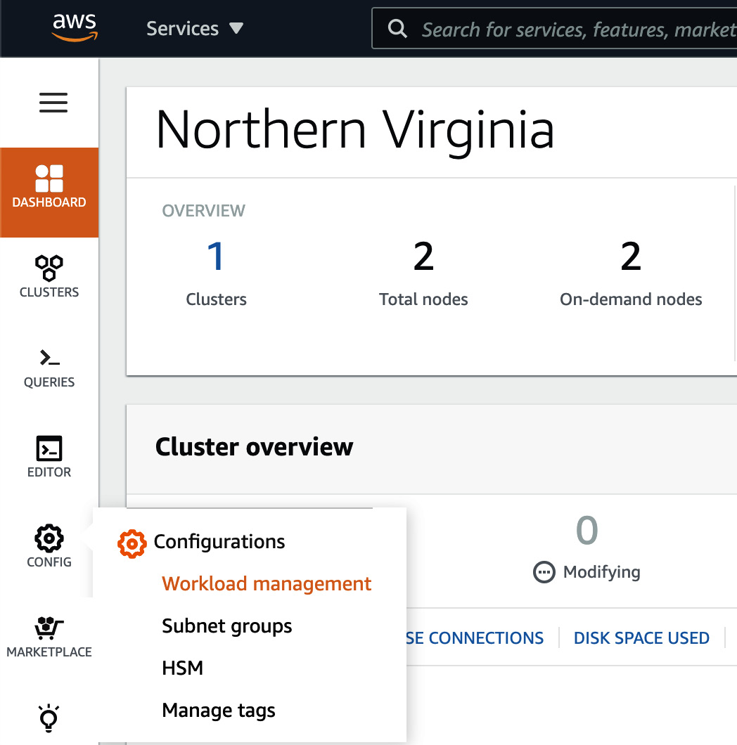
Figure 7.11 – Navigating Workload Management on the AWS Redshift Console
- On the Workload management page, we will need to create a new parameter group by clicking the Create button:

Figure 7.12 – Configuring a new parameter group
- A Create parameter group pop-up will open. Enter a Parameter group name and Description. Click on Create to finish creating a new parameter group:

Figure 7.13 – Creating a new parameter group called custom-parameter-group
- By default, Automatic WLM is configured under Workload Management. Automatic WLM is recommended, and it calculates the optimal memory and concurrency for query queues.
- To create a new queue, click on Edit workload queues in the Workload queues section. On the Modify workload queues: custom-parameter-group page, click on Add queue.
- You can configure the queue name by replacing the Queue 1 string and configuring other settings, such as Concurrency scaling mode between auto and off and Query priority between 5 levels ranging from lowest to highest. Additionally, you can include User groups or Query groups that need to be routed to this specific queue.
For example, we created an ETL queue with concurrency scaling disabled and query priority set to Normal. The user groups for data_engineers and query groups for load and transform will be routed to this queue:
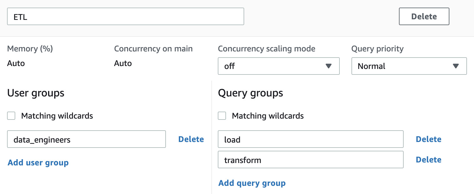
Figure 7.14 – Configuring the ETL queue on the parameter group
- You can repeat step 7 to create a total of 8 queues.
- You can create Query monitoring rules by either selecting Add rule from template or Add custom rule. This allows you to perform the log, abort, or change query priority action based on the predicates for the given query monitoring metrics.
For example, here, we created a rule to abort the query if it returns more than 100 million rows:
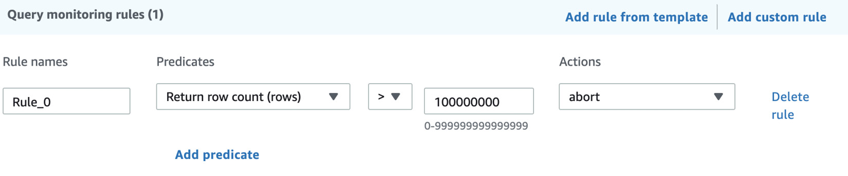
Figure 7.15 – Configuring a query monitoring rule
- To finish configuring the WLM settings, browse to the bottom of the page and click Save.
- To apply the new WLM settings to the cluster, browse to CLUSTERS and click the checkbox besides the Amazon Redshift cluster that you want to apply the new WLM settings to. Go to Actions and select Modify:
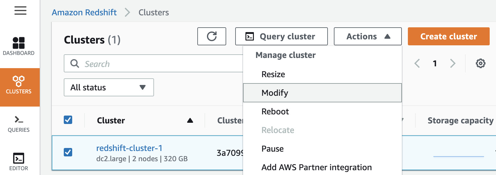
Figure 7.16 – Applying custom-parameter-group to your cluster
- Under the Modify cluster page, browse to the second set of Database configurations. Click the Parameter groups dropdown and select the newly created parameter group.
- Go to the bottom of the page and select Modify cluster. The changes are in the queue and applied once the cluster is rebooted.
- To reboot the cluster at an appropriate time that suits the business, click the checkbox besides the Amazon Redshift cluster, go to Actions, and select Reboot. A pop-up will appear to confirm the reboot. Select Reboot cluster.
How it works…
Amazon WLM's settings allows you to set up workload priorities and the concurrency of different types of workloads that run on an Amazon Redshift cluster. In addition, we have Auto WLM (recommended), which manages short query acceleration, memory allotment, and concurrency automatically. Using manual WLM, you can configure the memory and concurrency values for your workloads, if needed (not recommended).
Utilizing Concurrency Scaling
The Concurrency Scaling feature provided by Amazon Redshift allows you to support concurrent users and queries for steady query performance. Amazon Redshift utilizes resources that are available in a cluster to maximize throughput for analytical queries. Hence, when multiple queries are to be executed at the same time, Amazon Redshift will utilize workload management (WLM) to execute a few queries at a time so that they complete as soon as possible and don't take up the rest of the queries. This is done instead of you having to run all the queries for longer.
When the Concurrency Scaling feature is turned on, Amazon Redshift can instantly bring up additional redundant clusters to execute the queued-up queries and support burst traffic in the data warehouse. The redundant clusters are automatically shut down once the queries complete/there are no more queries waiting in the queue.
Getting ready
To complete this recipe, you will need the following:
- An Amazon Redshift cluster deployed in AWS region eu-west-1. You will also need the retail system dataset from the Loading data from Amazon S3 using COPY recipe in Chapter 3, Loading and Unloading Data.
- Amazon Redshift cluster master user credentials.
- Access to any SQL interface, such as a SQL client or the Amazon Redshift Query Editor.
- Install the par_psql client tool (https://github.com/gbb/par_psql) and psql https://docs.aws.amazon.com/redshift/latest/mgmt/connecting-from-psql.html on a Linux machine that can connect to an Amazon Redshift cluster.
How to do it…
In this recipe, we will be using the par_psql (https://github.com/gbb/par_psql) tool to execute parallel queries on Amazon Redshift to simulate concurrent workloads. Let's get started:
- Navigate to the AWS Amazon Redshift console and go to Amazon Redshift > Clusters > your Amazon Redshift Cluster. Click on the Properties tab and scroll down to Database configurations, as shown in the following screenshot:

Figure 7.17 – Database configurations
- Select the Parameter group property associated with the Amazon Redshift cluster.
- Click on the Parameter group property associated with the cluster.
- Verify that max_concurrency_scaling_clusters has been set to > =1 and that Workload queues has Concurrency scaling mode set to auto, as shown here:

Figure 7.18 – Workload queues
- Update Concurrency scaling mode to auto in Workload Queues.
For a step-by-step guide to setting up the Concurrency Scaling feature, please refer to the Managing workload management (WLM) recipe of this chapter.
- Download the par_psql script from https://github.com/PacktPublishing/Amazon-Redshift-Cookbook/blob/master/Chapter07/conc_scaling.sql and copy it into the path where par_psql has been installed. This script uses the retail system dataset, which we mentioned in the Getting started section.
- Execute the following command using the SQL client to capture the test's starttime:
select sysdate as starttime
Here is the expected output:
starttime
2020-12-04 16:10:43
- Execute the following command on the Linux box to simulate 100 concurrent query runs:
export PGPASSWORD=[PASSWORD]
./par_psql --file=conc_scaling.sql -h [YOUR AMAZON REDSHIFT HOST] -p [PORT] -d [DATABASE_NAME] -U [USER_NAME]
- Wait until all the queries have completed. Execute the following query to analyze the query execution. Do this by replacing [starttime] with the value corresponding to the datetime at the start of the script's execution, before the following query:
SELECT w.service_class AS queue
, case when q.concurrency_scaling_status = 1 then 'Y' else 'N' end as conc_scaled
, COUNT( * ) AS queries
, SUM( q.aborted ) AS aborted
, SUM( ROUND( total_queue_time::NUMERIC / 1000000,2 ) ) AS queue_secs
, SUM( ROUND( total_exec_time::NUMERIC / 1000000,2 ) ) AS exec_secs
FROM stl_query q
JOIN stl_wlm_query w
USING (userid,query)
WHERE q.userid > 1
AND q.starttime > '[starttime]'
GROUP BY 1,2
ORDER BY 1,2;
Here is the expected output:
queue | conc_scaled | queries | aborted | queue_secs | exec_secs
-------+-------------+---------+---------+------------+-----------
9 | N | 75 | 0 | 3569.83 | 31.24
9 | Y | 25 | 0 | 0.0| 10.97
As we can see, Amazon Redshift was able to take advantage of the Concurrency Scaling feature to execute 25% of the queries on the burst cluster.
How it works…
Concurrency Scaling allows users see the most current data, independent of whether the queries execute the main cluster or a Concurrency Scaling cluster. When Concurrency Scaling is used for peak workloads, you will be charged additional cluster time, but only for when they're used. Concurrency Scaling is enabled at a WLM queue, and eligible queries are sent to perform Concurrency Scaling when the concurrency in the queue exceeds the defined values, to ensure the queries do not wait. You can find more details about the queries that are eligible for Concurrency Scaling here: https://docs.aws.amazon.com/redshift/latest/dg/concurrency-scaling.html.
Optimizing Spectrum queries
Amazon Redshift Spectrum allows you to extend your Amazon Redshift data warehouse so that it can use SQL queries on data that is stored in Amazon S3. Optimizing Amazon Redshift Spectrum queries allows you to gain optimal throughput for SQL queries, as well as saving costs associated with them. In this recipe, we will learn how to gain insights into the performance of Spectrum-based queries and optimize them.
Getting ready
To complete this recipe, you will need the following:
- An IAM user with access to Amazon Redshift and Amazon S3.
- An Amazon Redshift cluster deployed in AWS region eu-west-1.
- Amazon Redshift cluster master user credentials.
- Access to any SQL interface, such as a SQL client or the Amazon Redshift Query Editor.
- An IAM role attached to an Amazon Redshift cluster that can access Amazon S3. We will reference it in this recipe as [Your-Redshift_Role].
- An AWS account number. We will reference it in this recipe as [Your-AWS_Account_Id].
How to do it…
In this recipe, we will use the Amazon.com customer product reviews dataset (refer to Chapter 3, Loading and Unloading Data) to demonstrate how to gain insight into Spectrum's SQL performance and tune it:
- Open any SQL client tool and connect to the Amazon Redshift cluster. Create a schema that points to the reviews dataset by using the following command, remembering to replace the [Your-AWS_Account_Id] and [Your-Redshift_Role] values with your own:
CREATE external SCHEMA reviews_ext_schema
FROM data catalog DATABASE 'reviews_ext_schema'
iam_role 'arn:aws:iam::[Your-AWS_Account_Id]:role/[Your-Redshift_Role]'
CREATE external DATABASE if not exists;
- Using the reviews dataset, create a parquet version of the external tables by using the following command:
CREATE external TABLE reviews_ext_schema.amazon_product_reviews_parquet(
marketplace varchar(2),
customer_id varchar(32),
review_id varchar(24),
product_id varchar(24),
product_parent varchar(32),
product_title varchar(512),
star_rating int,
helpful_votes int,
total_votes int,
vine char(1),
verified_purchase char(1),
review_headline varchar(256),
review_body varchar(max),
review_date date,
year int)
stored as parquet
location 's3://packt-redshift-cookbook/reviews_parquet/';
- Using the reviews dataset, create a plain text file (tab-delimited) version of the external tables by using the following command:
CREATE external TABLE reviews_ext_schema.amazon_product_reviews_tsv(
marketplace varchar(2),
customer_id varchar(32),
review_id varchar(24),
product_id varchar(24),
product_parent varchar(32),
product_title varchar(512),
star_rating int,
helpful_votes int,
total_votes int,
vine char(1),
verified_purchase char(1),
review_headline varchar(256),
review_body varchar(max),
review_date date,
year int)
row format delimited
fields terminated by ' '
stored as textfile
location 's3://packt-redshift-cookbook/reviews_tsv/';
- Execute the following analytical queries to calibrate the throughputs. Take note of the parquet_query_id and tsv_query_id outputs:
SELECT verified_purchase,
SUM(total_votes) total_votes,
avg(helpful_votes) avg_helpful_votes,
count(customer_id) total_customers
FROM reviews_ext_schema.amazon_product_reviews_parquet
WHERE review_headline = 'Y'
GROUP BY verified_purchase;
select PG_LAST_QUERY_ID() as parquet_query_id;
SELECT verified_purchase,
SUM(total_votes) total_votes,
avg(helpful_votes) avg_helpful_votes,
count(customer_id) total_customers
FROM reviews_ext_schema.amazon_product_reviews_tsv
WHERE review_headline = 'Y'
GROUP BY verified_purchase;
select PG_LAST_QUERY_ID() as tsv_query_id;
- Analyze the performance of both these queries by using the following command, substituting [parquet_query_id] and [tsv_query_id] from the previous step:
select query, segment, elapsed as elapsed_ms, s3_scanned_rows, s3_scanned_bytes, s3query_returned_rows, s3query_returned_bytes, files
from svl_s3query_summary
where query in ([parquet_query_id], [tsv_query_id])
order by query,segment ;
Here is the expected output:
query,elapsed_ms,s3_scanned_rows,s3_scanned_bytes,s3query_returned_rows,s3query_returned_bytes,files
parquet_query_id 3000554 5906460 142428017 4 1917 10
tsv_query_id 9182604 5906460 2001945218 4 5222 10
As we can see, the .tsv version of the dataset took 9 seconds versus 3 seconds in parquet since it has to scan 2 GB of data; only 0.14 MB of the data has to be scanned when it's in parquet format, even though the content of the files was the same.
Having the data in a columnar format such as parquet improves the query's throughput. It also reduces the cost that's incurred with the query due to an optimal scan being performed on the dataset.
How it works…
Optimizing Amazon Redshift Spectrum queries works on the principle of reducing the Amazon S3 scan and pushed down operations as much as possible into the infinitely scalable Spectrum engine. This can be achieved by using the following techniques:
- Amazon Redshift Spectrum supports structured and semi-structured data formats such as AVRO, PARQUET, ORC, TEXTFILE, JSON, and so on, and using a columnar file format such as parquet or ORC can reduce I/O by reading only the needed columns.
- Compress the row format file, such as a textfile, with compression file such as .gzip, snappy or .bzip to save costs and gain faster performance.
- Use an optimal file size:
a. Avoid excessively small files (less than 1 MB).
b. Avoid large files (1 GB or more) if the file format can't be split; for example, .gzip/snappy compressed text files.
- Organize the files as partitions. Take advantage of partition pruning and saving costs with the query.
You can read more about optimization techniques here: https://aws.amazon.com/blogs/big-data/10-best-practices-for-amazon-redshift-spectrum/.