Search in book...
Toggle Font Controls
Create new playlist

Name your new playlist

Playlist description (optional)
Sign In

Email address

Password

Forgot Password?

or

Continue with Facebook

Continue with Google
Sign Up

Full Name

Email address

Confirm Email Address

Password

or

Continue with Facebook

Continue with Google

Chapter 9: Lake House Architecture

The lake house is an architectural pattern that makes data easily accessible across customers' analytics solutions, thereby preventing data silos. Amazon Redshift is the backbone of the lake house architecture—it allows enterprise customers to query data across data lakes, operational databases, and multiple data warehouses to build an analytics solution without having to move data in and out of these different systems. In this chapter, you will learn how you can leverage the lake house architecture to extend the data warehouse to services outside Amazon Redshift to build your solution, while taking advantage of the built-in integration. For example, you can use the Federated Query capability to join the operational data in your relational systems to historical data in Amazon Redshift to analyze a promotional trend.

The following recipes are discussed in this chapter:

Building a data lake catalog using Amazon Web Services (AWS) Lake Formation
Exporting a data lake from Amazon Redshift
Extending a data warehouse using Amazon Redshift Spectrum
Data sharing across multiple Amazon Redshift clusters
Querying operational sources using Federated Query

Technical requirements

Here are the technical requirements in order to complete the recipes in this chapter:

Access to the AWS Management Console.
AWS administrators should create an Identity and Access Management (IAM) user by following Recipe 1 – Creating an IAM user in the Appendix. This IAM user will be deployed to perform some of the recipes in this chapter.
AWS administrators should create an IAM role by following Recipe 3 – Creating an IAM Role for an AWS service in the Appendix. This IAM role will be deployed to perform some of the recipes in this chapter.
AWS administrators should deploy the AWS CloudFormation template (https://github.com/PacktPublishing/Amazon-Redshift-Cookbook/blob/master/Chapter09/chapter_9_CFN.yaml) to create two IAM policies:
a. An IAM policy attached to the IAM user that will give them access to Amazon Redshift, Amazon Elastic Compute Cloud (Amazon EC2), Amazon Simple Storage Service (Amazon S3), Amazon Simple Notification Service (Amazon SNS), Amazon CloudWatch, Amazon CloudWatch Logs, AWS Key Management Service (AWS KMS), AWS IAM, AWS CloudFormation, AWS CloudTrail, Amazon Relational Database Service (Amazon RDS), AWS Lake Formation, AWS Secrets Manager, and AWS Glue
b. An IAM policy attached to the IAM role that will allow the Amazon Redshift cluster to access Amazon S3, Amazon RDS, and AWS Glue
Attach an IAM role to the Amazon Redshift cluster by following Recipe 4 – Attaching an IAM Role to the Amazon Redshift cluster in the Appendix. Make a note of the IAM role name—we will refer to this in the recipes as [Your-Redshift_Role].
An Amazon Redshift cluster deployed in the eu-west-1 AWS Region.
Amazon Redshift cluster masteruser credentials.
Access to any Structured Query Language (SQL) interface such as a SQL client or the Amazon Redshift Query Editor.
An AWS account number—we will refer to this in the recipes as [Your-AWS_Account_Id].
An Amazon S3 bucket created in the eu-west-1 Region. We will refer to this in the recipes as [Your-Amazon_S3_Bucket].
The code files are referenced in the GitHub repository at https://github.com/PacktPublishing/Amazon-Redshift-Cookbook/tree/master/Chapter09.

Building a data lake catalog using AWS Lake Formation

The data lake design pattern has been widely adopted in the industry. Data lakes help to break data silos by allowing you to store all of your data in a single, unified place. You can collect the data from different sources and data can arrive at different frequencies—for example, clickstream data. The data format can be structured, unstructured, or semi-structured. Analyzing a unified view of the data allows you to derive more value and helps to derive more insight from the data to drive business value.

Your data lake should be secure and should meet your compliance requirements, with a centralized catalog that allows you to search and easily find data that is stored in the lake. One of the advantages of data lakes is that you can run a variety of analytical tools against them. You may also want to do new types of analysis on your data. For example, you may want to move from answering questions on what happened in the past to what is happening in real time, and using statistical models and forecasting techniques to understand and answer what could happen in the future. To do this, you need to incorporate machine learning (ML), big data processing, and real-time analytics. The pattern that allows you to integrate your analytics into a data lake is the lake house architecture. Amazon S3 object storage is used for centralized data lakes due to its scalability, high availability, and durability.

You can see an overview of the lake house architecture here:

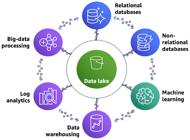
Figure 9.1 – Lake house architecture

Typical challenges and steps involved in building a data lake include the following:

Identifying sources and defining the frequency with which the data lake needs to be hydrated
Cleaning and cataloging the data
Centralizing the configuration and application of security policies
Integration of the data lake with analytical services that adhere to centralized security policies

Here is a representation of a lake house workflow moving data from raw format to analytics:

Figure 9.2 – Data workflow using the lake house architecture

The AWS Lake Formation service allows you to simplify the build, centralize management, and configure security policies. AWS Lake Formation leverages AWS Glue for cataloging, data ingestion, and data transformation.

In this recipe, you will learn how to use Lake Formation to hydrate the data lake from a relational database, catalog the data, and apply security policies.

Getting ready

To complete this recipe, you will need the following to be set up:

An IAM user with access to Amazon RDS, Amazon S3, and AWS Lake Formation.
An Amazon RDS MySQL database to create an RDS MySQL cluster (for more information, see https://aws.amazon.com/getting-started/hands-on/create-mysql-db/).
In this recipe, the version of the MySQL engine is 5.7.31.
A command line to connect to RDS MySQL (for more information, see https://docs.aws.amazon.com/AmazonRDS/latest/UserGuide/USER_ConnectToInstance.html).
This recipe is using an AWS EC2 Linux instance with a MySQL command line. Open the security group for the RDS MySQL database to allow connectivity from your client.

How to do it…

In this recipe, we will learn how to set up a data flow MySQL-based transactional database to be cataloged using a Lake Formation catalog and query it easily using Amazon Redshift:

Let's connect to the MySQLRDS database using the following command. Enter the password and it will connect you to the database:
mysql -h [yourMySQLRDSEndPoint] -u admin -p
We will create an ods database on MySQL and create a parts table in the ods database:
create database ods;
CREATE TABLE ods.part
(
  P_PARTKEY       BIGINT NOT NULL,
  P_NAME          VARCHAR(55),
  P_MFGR          VARCHAR(25),
  P_BRAND         VARCHAR(10),
  P_TYPE          VARCHAR(25),
  P_SIZE          INTEGER,
  P_CONTAINER     VARCHAR(10),
  P_RETAILPRICE   DECIMAL(18,4),
  P_COMMENT       VARCHAR(23)
);
On your client server, download the part.tbl file from https://github.com/PacktPublishing/Amazon-Redshift-Cookbook/blob/master/Chapter09/part.tbl to your local disk.
Now, we will load this file into the ods.part table on the MySQL database. This will load 20000 records into the parts table:
LOAD DATA LOCAL INFILE 'part.tbl'
    INTO TABLE ods.part
    FIELDS TERMINATED BY '|'
    LINES TERMINATED BY ' ';
Let's verify the record count loaded into the ods.part table:
MySQL [(none)]> select count(*) from ods.part;
+----------+
| count(*) |
+----------+
| 20000 |
+----------+
1 row in set (0.00 sec)
Navigate to AWS Lake Formation and click Get started:
Figure 9.3 – Navigating to Lake Formation
Now, let's set up the data lake location. Choose a register location:
Figure 9.4 – Data lake setup
Enter the location of the S3 bucket or folder in your account. If you do not have one, create a bucket on S3 in your account. Keep the default IAM role and click on Register location. With this, Lake Formation will manage the data lake location:
Figure 9.5 – Registering an Amazon S3 location in the data lake
Next, we will create a database that will serve as the catalog for the data in the data lake. Click on Create database, as shown here:
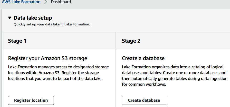
Figure 9.6 – Creating a database in Lake Formation
Use cookbook-data-lake as the database name. Select the s3 path that you registered in AWS Lake Formation. Select the Use only IAM access control for new tables in this database checkbox. Click on Create database:
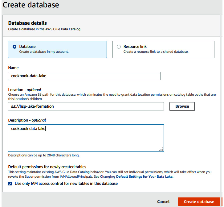
Figure 9.7 – Configuring the Lake Formation database
Now, we will hydrate the data lake from MySQL as the source. From the left menu, select Blueprint, and then click on Create blueprint.
Select Database snapshot, then right-click on Create a connection in AWS Glue to open a new tab:
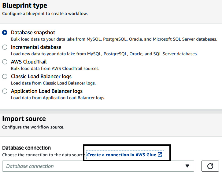
Figure 9.8 – Using a blueprint to create a database snapshot-based workflow
Set the following properties, as shown in Figure 9.9:
- Connection name—datalake-mysql
- Connection type—Amazon RDS
- Database engine—MySQL
Select Next:
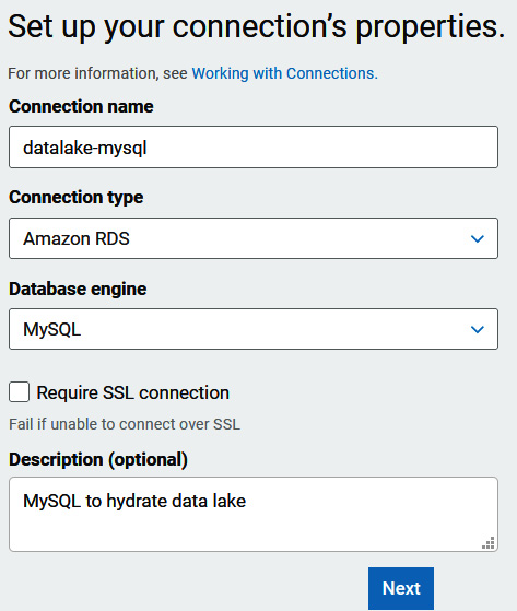
Figure 9.9 – Configuring Amazon RDS connection properties
Next, to set up access to your data store, set the following properties:
- Select an Instance name from the drop-down menu.
- Database name—ods.
- Username—admin.
- Enter the password you used to create the database.
Select Next and click Finish:
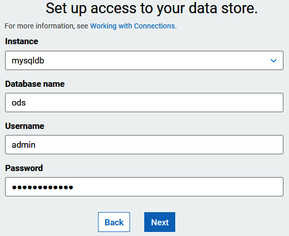
Figure 9.10 – Configuring the MySQL connection credentials
Select the datalake-mysql connection and select TestConnection. For the IAM role, use AWSGlueServiceRole-cookbook. Select TestConnection. This will take a few minutes. When it is successful, it will show a connected successfully to your instance message. If you run into issues with the connection setup, you can refer to the following Uniform Resource Locator (URL): https://aws.amazon.com/premiumsupport/knowledge-center/glue-test-connection-failed/.
Once successfully connected, you will see a connected successfully to your instance message, as shown here:
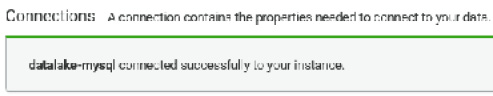
Figure 9.11 – Verifying a successful connection to the MySQL database
In AWS Lake Formation, set the following properties under Create blueprint:
a. For Database connection, from the drop-down menu select datalake-mysql.
b. For Source data path, enter ods/part:
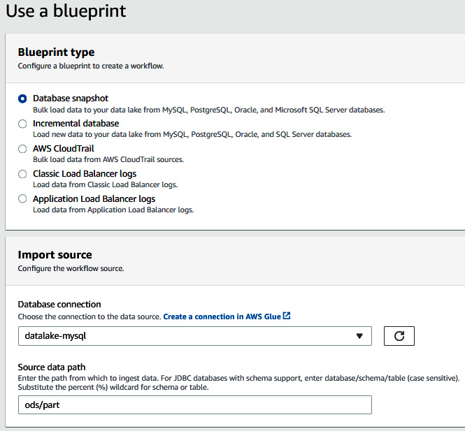
Figure 9.12 – Using a blueprint to create a database snapshot-based workflow
For Import target, select cookbook-data-lake for the Target database field. For Target location, specify your bucket path with mysql as the folder. We will unload the data from MySQL in Parquet format:
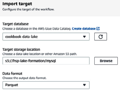
Figure 9.13 – Setting up the target for the data workflow
For Import frequency, select Run on demand:
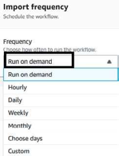
Figure 9.14 – Configuring the import frequency for the workflow
For Import options, specify the name of the workflow as hydrate-mysql. Under IAM role, use AWSGlueServiceRole-cookbook. For Table prefix, use mysql. Select Create:
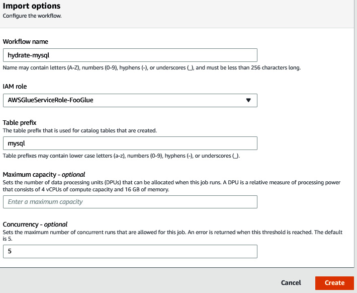
Figure 9.15 – Configuring import options for the workflow
When the workflow is created, select Workflows. Select Actions and start the workflow:
a. The workflow will crawl the mysql table metadata, which will catalog it in the cookbook-data-lake database.
b. It will then unload the data from the mysql ods.part table in Parquet format on the S3 location you provided.
c. Finally, it will crawl the Parquet data on S3 and create a table in the cookbook-data-lake database.
You can see an overview of this here:
Figure 9.16 – Crawling the target S3 Parquet bucket
To view the status of the workflow, click on Run Id. Then, select View graph:
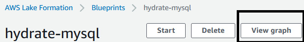
Figure 9.17 – Visualizing the data workflow
You can view the workflow steps and the corresponding status of the steps:
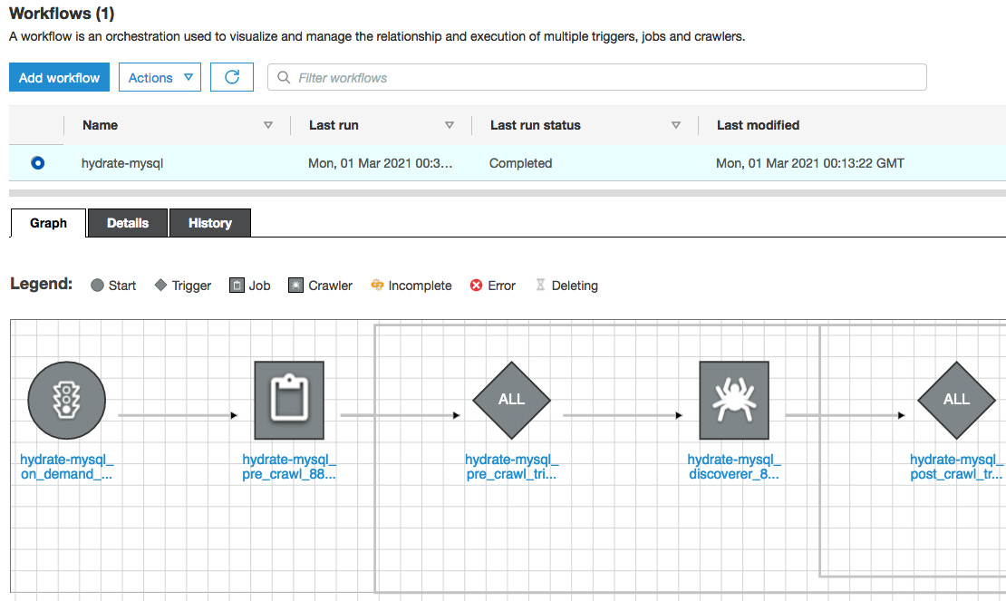
Figure 9.18 – Data workflow steps
On successful completion of the workflow, the Last run status field will be marked as COMPLETED:
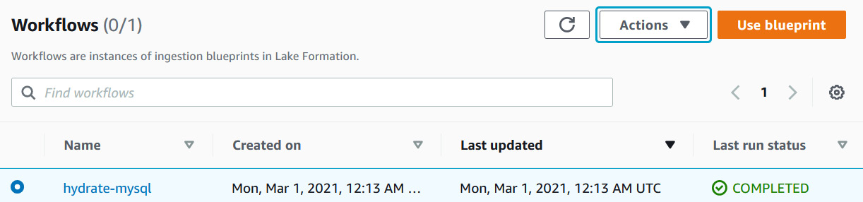
Figure 9.19 – Data workflow execution status
Let's now view the details of your first data lake. To view the tables created in your catalog, in the AWS Lake Formation console, from the left select Databases. Then, select cookbook-data-lake.
Select View tables:
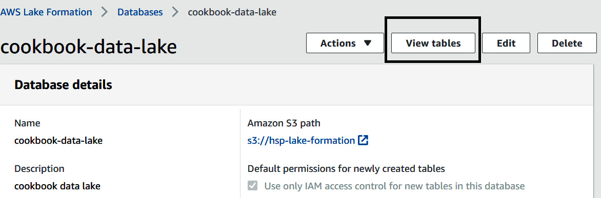
Figure 9.20 – Viewing tables created for the target
Let's verify the target dataset:
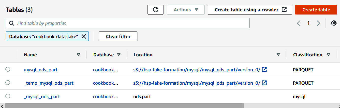
Figure 9.21 – Verifying the target dataset
To view the metadata of the Parquet unloaded data, select the mysql_ods_part table. This table is the metadata of the data. The crawler identified the column names and the corresponding data types:
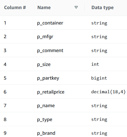
Figure 9.22 – Viewing metadata for the target
The classification is PARQUET and the table points to the location of s3, where the data resides:
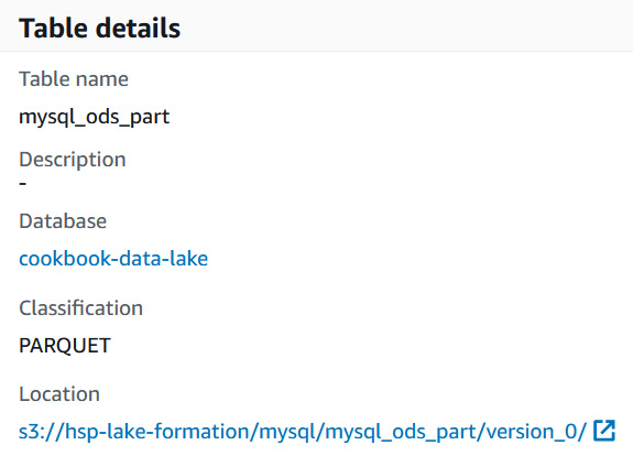
Figure 9.23 – Verifying the target table format
To view the unloaded files on S3, navigate to your S3 location:
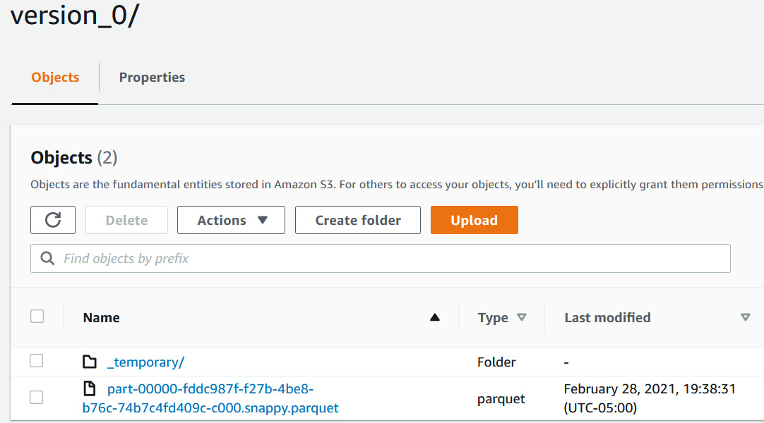
Figure 9.24 – Verifying the underlying Parquet files in Amazon S3
Going back to AWS Lake Formation, let's see how the permissions can be managed. In this step, we will use the mysql_ods_part table. Select the mysql_ods_part table, select Actions, and select Grant:
Figure 9.25 – Setting up permissions for the target dataset
AWS Lake Formation enables you to centralize the process of configuring access permissions to the IAM roles. Table-level and fine-grained access at column level can be granted and controlled from a centralized place:

Figure 9.26 – Administering the Lake Formation catalog

Later in the chapter, using the Extending a data warehouse using Amazon Redshift Spectrum recipe, you will learn how to query this data using Amazon Redshift.

How it works…

AWS Lake Formation simplifies the management and configuration of data lakes in a centralized place. AWS Glue's extract, transform, load (ETL) functionality, leveraging Python and Spark Shell, ML transform enables you to customize workflows to meet your needs. The AWS Glue/Lake Formation catalog integrates with Amazon Redshift for your data warehousing, Amazon Athena for ad hoc analysis, Amazon SageMaker for predictive analysis, and Amazon Elastic MapReduce (EMR) for big data processing.

Exporting a data lake from Amazon Redshift

Amazon Redshift empowers a lake house architecture, allowing you to query data within the data warehouse and data lake using Amazon Redshift Spectrum and also to export your data back to the data lake on Amazon S3, to be used by other analytical and ML services. You can store data in open file formats in your Amazon S3 data lake when performing the data lake export to integrate with your existing data lake formats.

Getting ready

To complete this recipe, you will need the following to be set up:

An IAM user with access to Amazon Redshift
An Amazon Redshift cluster deployed in the eu-west-1 AWS Region with the retail dataset created from Chapter 3, Loading and Unloading Data, using the Loading data from Amazon S3 using COPY recipe
Amazon Redshift cluster masteruser credentials
Access to any SQL interface such as a SQL client or the Amazon Redshift Query Editor
An AWS account number—we will refer to this in the recipes as [Your-AWS_Account_Id]
An Amazon S3 bucket created in the eu-west-1 Region—we will refer to this in the recipes as [Your-Amazon_S3_Bucket]
An IAM role attached to the Amazon Redshift cluster that can access Amazon S3—we will refer to this in the recipes as [Your-Redshift_Role]

How to do it…

In this recipe, we will use the sample dataset created from Chapter 3, Loading and Unloading Data, to write the data back to the Amazon S3 data lake:

Connect to the Amazon Redshift cluster using a client tool such as MySQL Workbench.
Execute the following analytical query to verify the sample dataset:
SELECT c_mktsegment,
       COUNT(o_orderkey) AS orders_count,
       SUM(l_quantity) AS quantity,
       COUNT(DISTINCT P_PARTKEY) AS parts_count,
       COUNT(DISTINCT L_SUPPKEY) AS supplier_count,
       COUNT(DISTINCT o_custkey) AS customer_count
FROM lineitem
  JOIN orders ON l_orderkey = o_orderkey
  JOIN customer c ON o_custkey = c_custkey
  JOIN dwdate
    ON d_date = l_commitdate
   AND d_year = 1992
  JOIN part ON P_PARTKEY = l_PARTKEY
  JOIN supplier ON L_SUPPKEY = S_SUPPKEY
GROUP BY c_mktsegment limit 5;
Here's the expected sample output:
c_mktsegment | orders_count |   quantity   | parts_count | supplier_count | customer_count
--------------+--------------+--------------+-------------+----------------+----------------
MACHINERY    |        82647 | 2107972.0000 |       75046 |          72439 |          67404
AUTOMOBILE   |        82692 | 2109248.0000 |       75039 |          72345 |          67306
HOUSEHOLD    |        82521 | 2112594.0000 |       74879 |          72322 |          67035
BUILDING     |        83140 | 2115677.0000 |       75357 |          72740 |          67411
FURNITURE    |        83405 | 2129150.0000 |       75759 |          73048 |          67876
Create a schema to point to the data lake using the following command, by replacing the [Your-AWS_Account_Id] and [Your-Redshift_Role] values:
CREATE external SCHEMA datalake_ext_schema
FROM data catalog DATABASE 'datalake_ext_schema'
iam_role 'arn:aws:iam::[Your-AWS_Account_Id]:role/[Your-Redshift_Role] '
CREATE external DATABASE if not exists;
Create an external table that will be used to export the dataset:
CREATE external TABLE datalake_ext_schema.order_summary
  (c_mktsegment VARCHAR(10),
   orders_count BIGINT,
   quantity numeric(38,4),
   parts_count BIGINT,
   supplier_count BIGINT,
   customer_count BIGINT
   )
STORED
AS
PARQUET LOCATION
's3://[Your-Amazon_S3_Bucket]/order_summary/';
Note
You are able to specify the output data format as PARQUET. You can use any of the supported data formats—see https://docs.aws.amazon.com/redshift/latest/dg/c-spectrum-data-files.html for more information.
Use the results of the preceding analytical query to export the data into the external table that will be stored in Parquet format in Amazon S3 using the following command:
INSERT INTO datalake_ext_schema.order_summary
SELECT c_mktsegment,
       COUNT(o_orderkey) AS orders_count,
       SUM(l_quantity) AS quantity,
       COUNT(DISTINCT P_PARTKEY) AS parts_count,
       COUNT(DISTINCT L_SUPPKEY) AS supplier_count,
       COUNT(DISTINCT o_custkey) AS customer_count
FROM lineitem
  JOIN orders ON l_orderkey = o_orderkey
  JOIN customer c ON o_custkey = c_custkey
  JOIN dwdate
    ON d_date = l_commitdate
   AND d_year = 1992
  JOIN part ON P_PARTKEY = l_PARTKEY
  JOIN supplier ON L_SUPPKEY = S_SUPPKEY
GROUP BY c_mktsegment;
You can now verify the results of the export using the following command:
select * from datalake_ext_schema.order_summary limit 5;
Here's the expected sample output:
c_mktsegment | orders_count |   quantity   | parts_count | supplier_count | customer_count
--------------+--------------+--------------+-------------+----------------+----------------
HOUSEHOLD    |        82521 | 2112594.0000 |       74879 |          72322 |          67035
MACHINERY    |        82647 | 2107972.0000 |       75046 |          72439 |          67404
FURNITURE    |        83405 | 2129150.0000 |       75759 |          73048 |          67876
BUILDING     |        83140 | 2115677.0000 |       75357 |          72740 |          67411
AUTOMOBILE   |        82692 | 2109248.0000 |       75039 |          72345 |          67306
In addition, you are also able to inspect the s3://[Your-Amazon_S3_Bucket]/order_summary/ Amazon S3 location for the presence of Parquet files, as shown here:
$ aws s3 ls s3://[Your-Amazon_S3_Bucket]/order_summary/
Here is the expected output:
2021-03-02 00:00:11       1588 20210302_000002_331241_25860550_0002_part_00.parquet
2021-03-02 00:00:11       1628 20210302_000002_331241_25860550_0013_part_00.parquet
2021-03-02 00:00:11       1581 20210302_000002_331241_25860550_0016_part_00.parquet
2021-03-02 00:00:11       1581 20210302_000002_331241_25860550_0020_part_00.parquet

The preceding sample output shows a list of all the Parquet files underlying the external table.

Extending a data warehouse using Amazon Redshift Spectrum

Amazon Redshift Spectrum allows Amazon Redshift customers to query data directly from an Amazon S3 data lake. This allows us to combine data warehouse data with data lake data, which makes use of open source file formats such as Parquet, comma-separated values (CSV), Sequence, Avro, and so on. Amazon Redshift Spectrum is a serverless solution, so customers don't have to provision or manage it. It allows customers to perform unified analytics on data in an Amazon Redshift cluster and data in an Amazon S3 data lake, and easily create insights from disparate datasets.

Getting ready

To complete this recipe, you will need the following to be set up:

An IAM user with access to Amazon Redshift
An Amazon Redshift cluster deployed in the eu-west-1 AWS Region with the retail dataset created from Chapter 3, Loading and Unloading Data, using the Loading data from Amazon S3 using COPY recipe
Amazon Redshift cluster masteruser credentials
Access to any SQL interface such as a SQL client or the Amazon Redshift Query Editor
An AWS account number—we will refer to this in the recipes as [Your-AWS_Account_Id]
An Amazon S3 bucket created in the eu-west-1 Region—we will refer to this in the recipes as [Your-Amazon_S3_Bucket]
An IAM role attached to the Amazon Redshift cluster that can access Amazon S3 and AWS Glue—we will refer to this in the recipes as [Your-Redshift_Role]

How to do it…

In this recipe, we will create external table in an external schema, and query data directly from Amazon S3 using Amazon Redshift:

Connect to the Amazon Redshift cluster using a client tool such as MySQL Workbench.
Execute the following query to create an external schema, by replacing the [Your-AWS_Account_Id] and [Your-Redshift_Role] values:
create external schema packt_spectrum
from data catalog
database 'packtspectrumdb'
iam_role 'arn:aws:iam::[Your-AWS_Account_Id]:role/[Your-Redshift_Role]'
create external database if not exists;
Execute the following command to copy data from the Packt S3 bucket to your S3 bucket using the following command, by replacing [Your-Amazon_S3_Bucket]:
aws cp s3://packt-redshift-cookbook/spectrum/sales s3://[Your-Amazon_S3_Bucket]/spectrum/sales --recursive
Execute the following query to create an external table, by replacing [Your-Amazon_S3_Bucket]:
create external table packt_spectrum.sales(
salesid integer,
listid integer,
sellerid integer,
buyerid integer,
eventid integer,
dateid smallint,
qtysold smallint,
pricepaid decimal(8,2),
commission decimal(8,2),
saletime timestamp)
row format delimited
fields terminated by ' '
stored as textfile
location 's3://[Your-Amazon_S3_Bucket]/spectrum/sales/'
table properties ('numRows'='172000');
Execute the following command to query data in S3 directly from Amazon Redshift:
select count(*) from packt_spectrum.sales; --
expected sample output –
count
------
172462
Execute the following command to create a table locally in Amazon Redshift:
create table packt_event(
eventid integer not null distkey,
venueid smallint not null,
catid smallint not null,
dateid smallint not null sortkey,
eventname varchar(200),
starttime timestamp);
Execute the following command to load data in the event table, by replacing the [Your-AWS_Account_Id] and [Your-Redshift_Role] values:
copy packt_event from 's3://packt-redshift-cookbook/spectrum/event/allevents_pipe.txt'
iam_role 'arn:aws:iam::[Your-AWS_Account_Id]:role/[Your-Redshift_Role]
delimiter '|' timeformat 'YYYY-MM-DD HH:MI:SS' Region 'us-east-1';
Execute the following query to join the data across the Redshift local table and the Spectrum table:
SELECT top 10 packt_spectrum.sales.eventid,
       SUM(packt_spectrum.sales.pricepaid)
FROM packt_spectrum.sales,
     packt_event
WHERE packt_spectrum.sales.eventid = packt_event.eventid
AND   packt_spectrum.sales.pricepaid > 30
GROUP BY packt_spectrum.sales.eventid
ORDER BY 2 DESC;
Here's the expected output:
eventid | sum
--------+---------
    289 | 51846.00
   7895 | 51049.00
   1602 | 50301.00
    851 | 49956.00
   7315 | 49823.00
   6471 | 47997.00
   2118 | 47863.00
    984 | 46780.00
   7851 | 46661.00
   5638 | 46280.00

Now, Amazon Redshift is able to join the external and local tables to produce the desired results.

Data sharing across multiple Amazon Redshift clusters

Amazon Redshift RA3 clusters decouple storage and compute, and provide the ability to scale either of them independently. The decoupled storage allows for data to be read by different consumer clusters that allow workload isolation. The data producer cluster controls access to the data that is shared. This feature opens up the possibility to set up a flexible multi-tenant system—for example, within an organization, data produced by a business unit can be shared with any of the different teams such as marketing, finance, data science, and so on that can be independently consumed using their own Amazon Redshift clusters.

Getting ready

To complete this recipe, you will need the following:

An IAM user with access to Amazon Redshift
Two separate two-node Amazon Redshift ra3.xlplus clusters deployed in the eu-west-1 AWS Region:
a. The first cluster should be deployed with the retail sample dataset from Chapter 3, Loading and Unloading Data. This cluster will be called the Producer Amazon Redshift cluster, where data will be shared from (outbound). Note down the namespace of this cluster—this can be found by running a SELECT current_namespace command. Let's say this cluster namespace value is [Your_Redshift_Producer_Namespace].
b. The second cluster can be an empty cluster. This cluster will be called the Consumer Amazon Redshift cluster, where data will be consumed (inbound). Note down the namespace of this cluster—this can be found by running a SELECT current_namespace command. Let's say this cluster namespace value is [Your_Redshift_Consumer_Namespace].
Access to any SQL interface such as a SQL client or the Amazon Redshift Query Editor

How to do it…

In the recipe, we will use the Producer Amazon Redshift RA3 cluster, with the sample dataset to be shared with the consumer cluster:

Connect to the Producer Amazon Redshift cluster using a client tool such as MySQL Workbench.
Execute the following analytical query to verify the sample dataset:
SELECT DATE_TRUNC('month',l_shipdate),
       SUM(l_quantity) AS quantity
FROM lineitem
WHERE l_shipdate BETWEEN '1992-01-01' AND '1992-06-30'
GROUP BY DATE_TRUNC('month',l_shipdate);
--Sample output dataset
     date_trunc      |    quantity
---------------------+----------------
1992-05-01 00:00:00 | 196639390.0000
1992-06-01 00:00:00 | 190360957.0000
1992-03-01 00:00:00 | 122122161.0000
1992-02-01 00:00:00 |  68482319.0000
1992-04-01 00:00:00 | 166017166.0000
1992-01-01 00:00:00 |  24426745.0000
Create a datashare and add the lineitem table so that it can be shared with the consumer cluster using the following command, replacing [Your_Redshift_Consumer_Namespace] with consume cluster namespace:
CREATE DATASHARE SSBDataShare;
ALTER DATASHARE SSBDataShare ADD TABLE lineitem;
GRANT USAGE ON DATASHARE SSBDataShare TO NAMESPACE ' [Your_Redshift_Consumer_Namespace]';
Execute the following command to verify that data sharing is available:
SHOW DATASHARES;
Here's the expected output:
owner_account,owner_namespace,sharename,shareowner,share_type,createdate,publicaccess
123456789012,redshift-cluster-data-share-1,ssbdatashare,100,outbound,2021-02-26 19:03:16.0,false
Connect to the Amazon Redshift Consumer cluster using a client tool such as MySQL Workbench. Execute the following command:
DESC DATASHARE ssbdatashare OF NAMESPACE [Your_Redshift_Producer_Namespace];
Here's the expected output:
producer_account | producer_namespace | share_type | share_name | object_type | object_name
-------------------+--------------------------------------+------------+------------+-------------+---------------------------------
123456789012 | [Your_Redshift_Producer_Namespace]| INBOUND | ssbdatashare | table | public.lineitem
Create local databases that reference the datashares using the following command:
CREATE DATABASE ssb_db FROM DATASHARE ssbdatashare OF NAMESPACE [Your_Redshift_Producer_Namespace];
Create an external schema that references the ssb_db datashare database by executing the following command:
CREATE EXTERNAL SCHEMA ssb_schema FROM REDSHIFT DATABASE 'ssb_db' SCHEMA 'public';
Verify the datashare access to the linetime table using a full qualification, as follows:
SELECT DATE_TRUNC('month',l_shipdate),
       SUM(l_quantity) AS quantity
FROM ssb_db.public.lineitem
WHERE l_shipdate BETWEEN '1992-01-01' AND '1992-06-30'
GROUP BY DATE_TRUNC('month',l_shipdate);
Here's the sample dataset:
     date_trunc      |    quantity
---------------------+----------------
1992-05-01 00:00:00 | 196639390.0000
1992-06-01 00:00:00 | 190360957.0000
1992-03-01 00:00:00 | 122122161.0000
1992-02-01 00:00:00 |  68482319.0000
1992-04-01 00:00:00 | 166017166.0000
1992-01-01 00:00:00 |  24426745.0000

As you can see from the preceding code snippet, the data that is shared by the producer cluster is now is available for querying in the consumer cluster.

How it works…

With Amazon Redshift, you can share data at different levels. These levels include databases, schemas, tables, views (including regular, late-binding, and materialized views), and SQL user-defined functions (UDFs). You can create multiple datashares for a given database. A datashare can contain objects from multiple schemas in the database on which sharing is created.

By having this flexibility in sharing data, you get fine-grained access control. You can tailor this control for different users and businesses that need access to Amazon Redshift data. Amazon Redshift provides transactional consistency on all producer and consumer clusters and shares up-to-date and consistent views of the data with all consumers. You can also use SVV_DATASHARES, SVV_DATASHARE_CONSUMERS, and SVV_DATASHARE_OBJECTS to view datashares, the objects within the datashares, and the datashare consumers.

Querying operational sources using Federated Query

Amazon Redshift Federated Query enables unified analytics across databases, data warehouses, and data lakes. With the Federated Query feature in Amazon Redshift, you can query live data across from Amazon RDS and Aurora PostgreSQL databases. For example, you might have an up-to-date customer address data that you might want to join with historical order data to enrich your reports—this can be easily joined up using the Federated Query feature.

Getting ready

To complete this recipe, you will need the following:

An IAM user with access to Amazon Redshift, AWS Secrets Manager, and Amazon RDS.
An Amazon Redshift cluster deployed in the eu-west-1 AWS Region with the retail sample dataset from Chapter 3, Loading and Unloading Data.
An Amazon Aurora serverless PostgreSQL database. Create an RDS PostgreSQL cluster (see https://aws.amazon.com/getting-started/hands-on/building-serverless-applications-with-amazon-aurora-serverless/ for more information on this). Launch this in the same virtual private cloud (VPC) as your Amazon Redshift cluster.
Access to any SQL interface such as a SQL client or the Amazon Redshift Query Editor.
An IAM role attached to the Amazon Redshift cluster that can access Amazon RDS—we will refer to this in the recipes as [Your-Redshift_Role].
An AWS account number—we will refer to this in the recipes as [Your-AWS_Account_Id].

How to do it…

In this recipe, we will use an Amazon Aurora serverless PostgreSQL database as the operational data store to federate with Amazon Redshift:

Let's connect to the Aurora PostgreSQL database using a Query Editor. Navigate to the Amazon RDS landing page and choose Query Editor.
Choose an instance from the RDS instance dropdown. Enter a username and a password. For the Database field, enter postgres, and then select Connect to database:
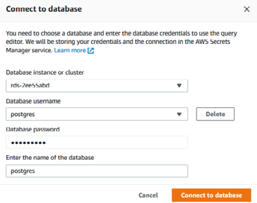
Figure 9.27 – Configuring the Amazon Aurora PostgreSQL database
Copy and paste the SQL script available at https://github.com/PacktPublishing/Amazon-Redshift-Cookbook/blob/master/Chapter09/aurora_postgresql_orders_insert.sql into the editor. Select Run:
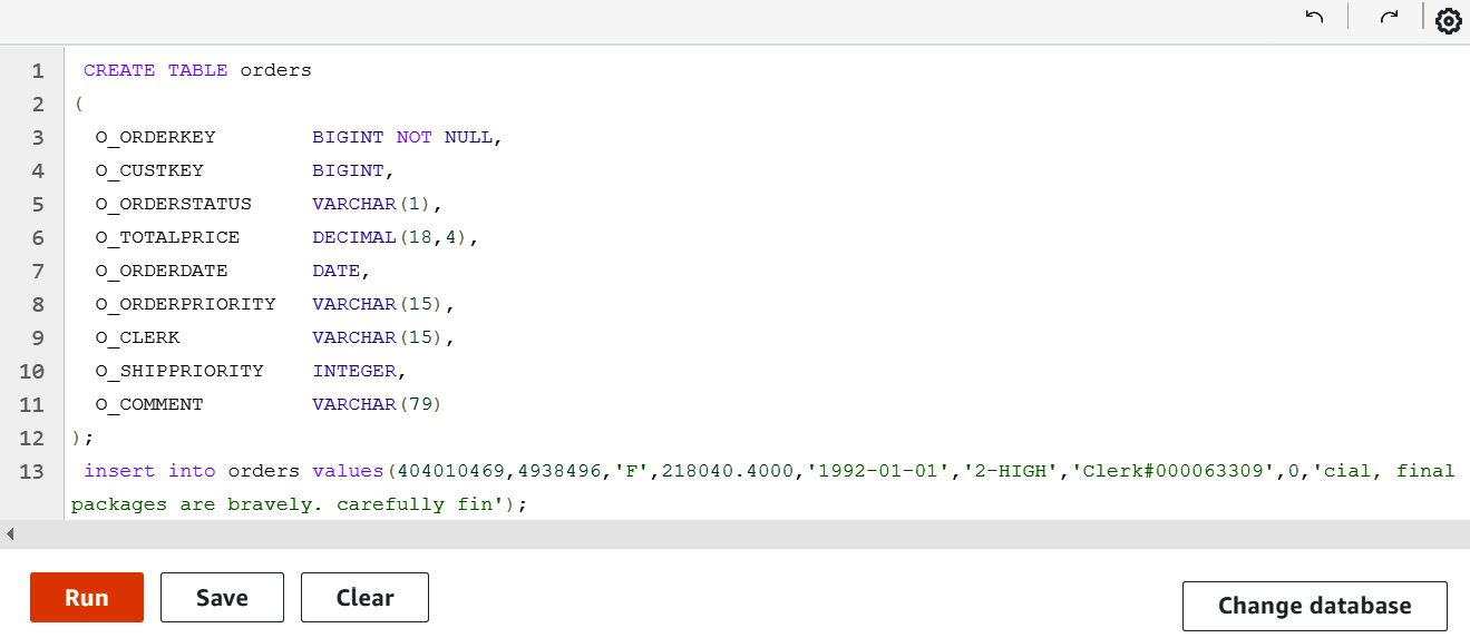
Figure 9.28 – Creating the orders tables
We will now create an Aurora PostgreSQL database secret using AWS Secrets Manager to store the user ID and password.
Navigate to the AWS Secrets Manager console. Choose Store a new secret.
Select Credentials for RDS database, then enter the username and password. Select your database instance and click Next:
Figure 9.29 – Setting up credentials for RDS
Enter the the name of aurora-pg/RedshiftCookbook for the secret. Click Next:
Figure 9.30 – Creating an Aurora PostgreSQL secret
Click Next, keep the defaults, and choose Store.
Select the newly created secret and copy the Amazon Resource Name (ARN) of the secret:
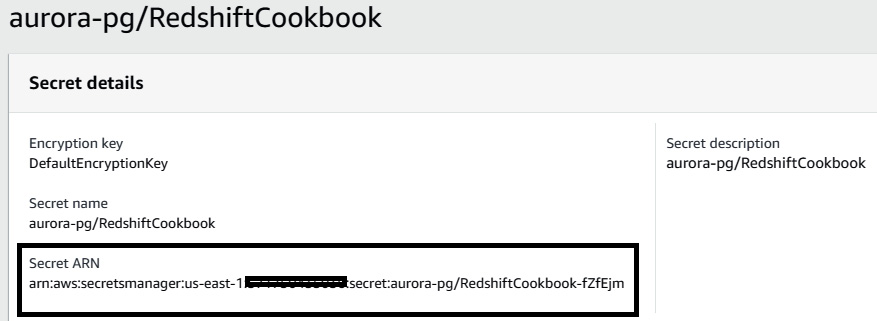
Figure 9.31 – Copying the Secret ARN value for the secret
To configure Amazon Redshift to federate with the Aurora PostgreSQL database, we need to attach an inline policy to the IAM role attached to your Amazon Redshift cluster to provide access to the secret created in the preceding steps. For this, navigate to the IAM console and select Roles.
Search for the correct role. Add the following inline policy. Replace [Your-AWS_Account_Id] with your AWS account number:
{
    "Version": "2012-10-17",
    "Statement": [
        {
            "Sid": "AccessSecret",
            "Effect": "Allow",
            "Action": [
                "secretsmanager:GetResourcePolicy",
                "secretsmanager:GetSecretValue",
                "secretsmanager:DescribeSecret",
                "secretsmanager:ListSecretVersionIds"
            ],
            "Resource": "arn:aws:secretsmanager:us-east-1:[Your-AWS_Account_Id]:secret:aurora-pg/RedshiftCookbook"
        },
        {
            "Sid": "VisualEditor1",
            "Effect": "Allow",
            "Action": [
                "secretsmanager:GetRandomPassword",
                "secretsmanager:ListSecrets"
            ],
            "Resource": "*"
        }
    ]
}
Let's set up Amazon Redshift to federate to the Aurora PostgreSQL database to query the orders' operational data. For this, connect to your Amazon Redshift cluster using an SQL client or the Query Editor from Amazon Redshift console.
Create an ext_postgres external schema on Amazon Redshift. Replace [AuroraClusterEndpoint] with the endpoint of the instance from your account for the Aurora PostgreSQL database. Replace the [Your-AWS_Account_Id] and [Your-Redshift-Role] values from your account. Also, replace [AuroraPostgreSQLSecretsManagerARN] with the value of the secret ARN from Step 9:
DROP SCHEMA IF EXISTS ext_postgres;
CREATE EXTERNAL SCHEMA ext_postgres
FROM POSTGRES
DATABASE 'postgres'
URI '[AuroraClusterEndpoint]'
IAM_ROLE 'arn:aws:iam::[Your-AWS_Account_Id]:role/[Your-Redshift-Role]'
SECRET_ARN '[AuroraPostgreSQLSecretsManagerARN]';
To list the external schemas, execute the following query:
select *
from svv_external_schemas;
To list the external schema tables, execute the following query:
select *
from svv_external_tables
where schemaname = 'ext_postgres';
To validate the configuration and setup of Federated Query from Amazon Redshift, let's execute a count query for the orders table in the Aurora PostgreSQL database:
select count(*) from ext_postgres.orders;
Here's the expected output:
1000
With Federated Query, you can join the external table with the Amazon Redshift local table:
SELECT O_ORDERSTATUS,
       COUNT(o_orderkey) AS orders_count
FROM ext_postgres.orders
    JOIN dwdate
    ON d_date = O_ORDERDATE
   AND d_year = 1992
GROUP BY O_ORDERSTATUS;
Here's the expected output:
o_orderstatus   orders_count
F            1000
You can also create a materialized view using Federated Query. A materialized view will be physicalized on Amazon Redshift. You can refresh the materialized view to get fresher data from your operational data store (ODS):
create materialized view public.live_orders as
SELECT O_ORDERSTATUS,
       COUNT(o_orderkey) AS orders_count
FROM ext_postgres.orders
    JOIN dwdate
    ON d_date = O_ORDERDATE
   AND d_year = 1992
GROUP BY O_ORDERSTATUS;

As observed, the materialized view can federate between the Aurora PostgreSQL and Amazon Redshift databases.

..................Content has been hidden....................

You can't read the all page of ebook, please click here login for view all page.

Table of Contents for Chapter 9: Lake House Architecture

Create new playlist

Sign In

Sign Up

Chapter 9: Lake House Architecture

Technical requirements

Building a data lake catalog using AWS Lake Formation

Getting ready

How to do it…

How it works…

Exporting a data lake from Amazon Redshift

Getting ready

How to do it…

Extending a data warehouse using Amazon Redshift Spectrum

Getting ready

How to do it…

Data sharing across multiple Amazon Redshift clusters

Getting ready

How to do it…

How it works…

Querying operational sources using Federated Query

Getting ready

How to do it…

Table of Contents for
Chapter 9: Lake House Architecture