13

TRANSMISSION-LINE NETWORKS

The previous chapters of this book have considered the analysis of uniform transmission lines that have one important restriction: All n + 1 conductors are parallel to each other. Numerous practical configurations consist of interconnections of these types of lines as illustrated in Figure 13.1(a). These practical configurations will be referred to as transmission-line networks. Lines may end in termination networks or may be interconnected by interconnection networks. Each transmission line of the network will be referred to as a tube after [1–3]. A convenient way of describing the overall network is with a graph as illustrated in Figure 13.1(b) [1,2,4]. The transmission lines are represented with single lines or branches of the graph. The termination networks are defined as a node having only one tube incident on it and are represented by rectangles. The interconnection networks are defined as a node having more than one tube incident on it and are represented by circles. The excitation for the network may be in the form of lumped sources in the termination or interconnection networks or it may be due to either distributed excitation from an incident electromagnetic field or a point excitation along the line as with the direct attachment of a lightning stroke. Point excitation of a tube as in the case of a direct attachment of a lightning stroke can be handled by characterizing the segments of the tube to the left and right of the excitation point with any of the following models and treating the point excitation as an interconnection network between these tube subsegments. Lumped sources in this interconnection network then represent this point excitation at the junction. Distributed excitation must be included in the overall characterization of the tube as described in Chapters 11 and 12, whereas lumped sources within the termination/interconnection networks are included in their description. The purpose of this chapter is to examine methods for characterizing these types of interconnected lines.

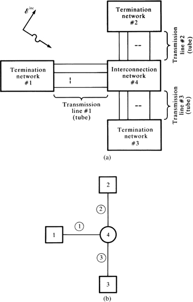
FIGURE 13.1 Illustration of a transmission-line network: (a) tube and network definitions and (b) representation with a graph.

Evidently, any method for characterizing this network seeks to (1) characterize each tube in some fashion as outlined in the previous chapters and (2) interconnect these tubes by enforcing the constraints on the line voltages and currents via Kirchhoff's laws and the element characteristics within the termination/interconnection networks. One obvious representation method is to use SPICE subcircuit models for the tubes developed in Chapters 8, 9, 11, and 12 and interconnect and/or terminate the nodes of those subcircuit models in the resulting SPICE code. This method is very straightforward using the program SPICEMTL.FOR or SPICEINC.FOR described in Appendix A to provide the SPICE subcircuit models of each tube. The advantages of this method are that (1) it is straightforward to implement and (2) dynamic as well as nonlinear loading and elements within the termination/interconnection networks such as diodes and transistors are already available in the SPICE code and can be readily used to build the termination/interconnection networks to complete the overall characterization. So a wide variety of practical terminations can be analyzed without the need for developing either the models of complicated elements or the numerical integration routines to give a time-domain analysis. The disadvantage of this method is that it is so far applicable only to lossless lines.

An approximate method is to use lumped-circuit iterative models of each tube such as the lumped-Pi or lumped-T models and use any lumped-circuit analysis program such as SPICE to analyze the resulting interconnection. Frequency-independent losses can be incorporated into this result, but the method is restricted to tubes that are electrically short. Time-domain results can again be reasonably approximated if the rise/fall times of the source waveforms are sufficiently longer than the tube one-way delays.

It is also possible to construct an exact model of the line using the frequency-domain admittance or impedance parameter characterizations of each tube [4, 5]. These methods have the advantage of simple construction of the overall equations that are to be solved to give the tube terminal voltages and currents. Losses such as skin-effect losses that vary as can be included by simply determining the frequency response of the network and converting to the time domain with the time-domain to frequency-domain (TDFD) transformation.

With the exception of the SPICE subcircuit method, all methods ultimately must face the problem of the systematic interconnection of the tube models. Computer implementation of the interconnection of the tubes for a large network is not a simple task and must be designed so that a user can easily and unambiguously describe the interconnections to the resulting computer code. Of course, all standard lumped-circuit analysis codes such as SPICE must address this problem of systematic and unambiguous implementation of the element interconnections via user input to the code, and the characterization of transmission-line networks is similar in that respect. Characterization of the tubes via the admittance parameters as in [4] was designed so that a systematic interconnection process will be affected. Another method is the use of the scattering parameters for the tubes [1,2]. This leads to the so-called BLT equations (apparently named for the authors). A similar modal decomposition method was described in [3].

All of the above methods must address both the frequency-domain and the time-domain analysis of the network. The time-domain analysis of the network can be obtained in the usual fashion using the TDFD transformation discussed earlier wherein the source waveform is decomposed into its spectral components and each component is passed through the previously computed frequency-domain transfer function. The time-domain result is the inverse Fourier transform of this. As before, the TDFD method can readily handle skin-effect losses that are difficult to characterize in the time domain, but it suffers from the fundamental restriction that the network must be linear, that is, the line and all terminations must be linear, since superposition is used.

13.1 REPRESENTATION OF LOSSLESS LINES WITH THE SPICE MODEL

Perhaps one of the more straightforward methods of characterizing and analyzing the crosstalk on transmission-line networks or the effect of incident fields is with the SPICE equivalent circuit developed in Chapters 8 and 9 or incident field illumination in Chapters 11 and 12. Each tube is characterized by its SPICE subcircuit model generated with the program SPICEMTL.FOR or SPICEINC.FOR described in Appendix A. These subcircuit models are then interconnected and the terminations added to produce the final SPICE model of the network. The method is straightforward using the above codes to generate the subcircuit models but is restricted to lossless tubes. Again, this method can handle, in a straightforward way, dynamic and/or nonlinear loads in the termination/interconnection networks.

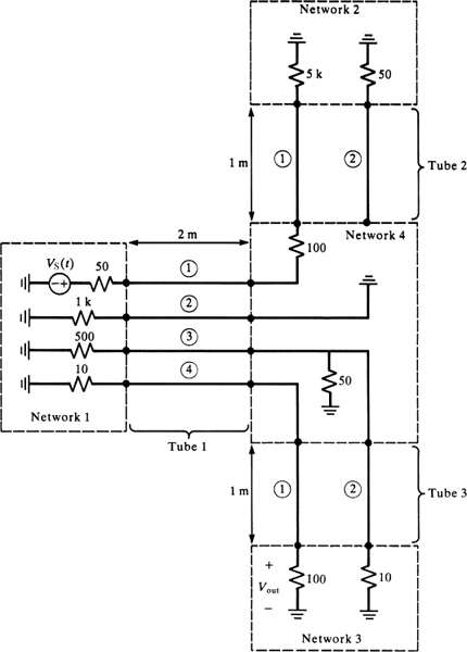
FIGURE 13.2 An example of a transmission-line network to illustrate and compare numerical results.

In order to illustrate the methods of this chapter, we will use the example shown in Figure 13.2. The network consists of three tubes. Tube #1 contains four wires, whereas tubes #2 and #3 contain two wires. All tubes will consist of bare wires above a ground plane as illustrated in Figure 13.3. Tube #1 is of length 2 m and tubes #2 and #3 are of length 1 m. The cable is suspended 1 cm above an infinite, perfectly conducting ground plane, and the wires have radii of 7.5 mils. A source, V_S(t), in network #1 drives line #1 of tube #1. This source is in the form of a ramp waveform with a rise time of 1 ns as shown in Figure 13.3(c). The tubes are terminated in various resistive terminations at termination networks #1, #2, and #3. Interconnection network #4 contains a variety of terminations, open circuit, short circuit, series impedance, shunt impedance, and direct connection, to illustrate the versatility of the method. The desired output will be the voltage, V_out(t), across the termination of wire #1 of tube #3 at termination network #3. The graph of this transmission-line network is shown in Figure 13.1(b). Each termination or interconnection network has the number of that node included within the symbol. The number of each tube is noted on that branch of the graph.

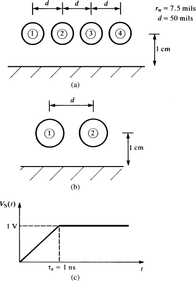
FIGURE 13.3 Cross-sectional dimensions of the tubes of the transmission-line network of Figure 13.2.

Figure 13.4 illustrates the resulting construction of the overall SPICE network with node numbering. The SPICE subcircuit models of the tubes are constructed using SPICEMTL.FOR, and the per-unit-length parameters are computed using WIDESEP.FOR.

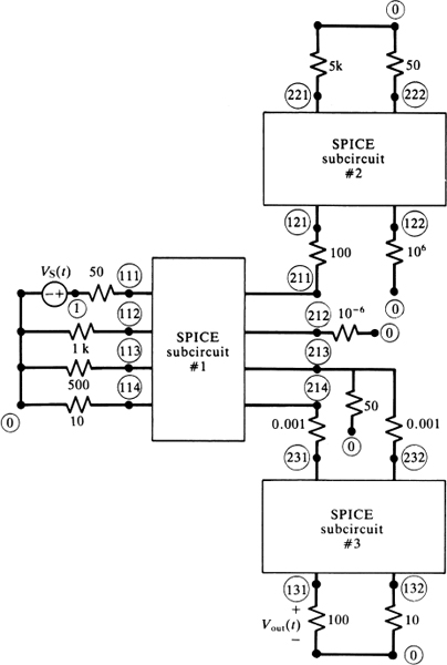
FIGURE 13.4 Illustration of the SPICE model of the transmission-line network of Figure 13.2.

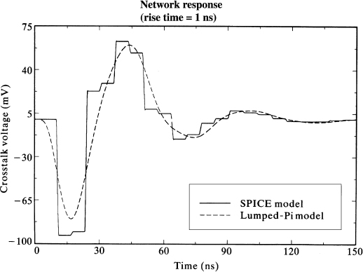
FIGURE 13.5 Comparison of crosstalk voltage at the termination of conductor #1 of tube #3 for the transmission-line network of Figure 13.2 for a rise time of 1 ns using the SPICE model and using one lumped-Pi section to represent each tube.

13.2 REPRESENTATION WITH LUMPED-CIRCUIT APPROXIMATE MODELS

The next method is to approximately characterize each tube with a lumped-circuit approximate structure such as a lumped-Pi structure. These characterizations are obtained using the SPICELPI.FOR code. The resulting overall SPICE model of the network is virtually identical to that of Figure 13.4 with the only exception being that the subcircuit models of the tubes are lumped-Pi structures. Figure 13.5 shows the comparison of the predictions of the output voltage, V_out(t), obtained with the SPICE model of Figure 13.4 and 1the lumped-Pi structure using only one lumped-Pi section to represent each tube. The correlation is obviously very poor due to the fact that the tube one-way delays are on the order of 3 ns and 6 ns that are not significantly smaller than the waveform rise time of 1 ns. Figure 13.6 shows this correlation for a rise time of 100 ns, which is much better.

13.3 REPRESENTATION VIA THE ADMITTANCE OR IMPEDANCE 2n-PORT PARAMETERS

The use of the admittance parameters to characterize the tubes was described in [4]. This leads to a straightforward way of incorporating the termination and interconnection networks, since we essentially need to simply add admittances in order to construct the admittance matrix of the overall network.

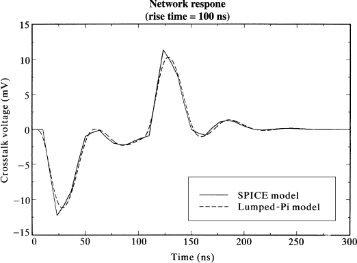
FIGURE 13.6 The predictions of Figure 13.5 for a rise time of 100 ns showing the adequacy of the lumped-Pi representation.

The frequency-domain chain parameters of a uniform line are

where and Î_FT are due to any incident field excitation of the line. The frequency-domain admittance parameters are derived in Section 7.5.5 of Chapter 7 from these to yield

where

Observe that the currents are defined as directed into each end of the tube. The admittance parameters show that the tube is reciprocal as it should be. The various parameters in these are as defined in Chapter 7, where the per-unit-length impedance and admittance parameters are diagonalized as

and the characteristic admittance matrix is

The only potential disadvantage to the admittance parameter description of the tubes is that the parameters do not exist for lossless lines and frequencies where the tube is a multiple of a half wavelength.

The tubes are characterized by the above admittance parameters with the following notation illustrated in Figure 13.7(a). Consider the ith tube connecting the jth network and the kth network at its endpoints. Denote the vector of currents and voltages at the ends of the tube as , , , and , where the subscript denotes the tube and the superscript denotes the network at that end:

The admittance parameters (13.2) and (13.3) become

where accounts for the effects of the incident field incident on tube i referred to the end at network j, whereas accounts for the effect of the incident field on tube i referred to the end at network k.

The characterization of the termination and interconnection networks must be general enough to include open and short circuits as well as lumped sources and impedances and direct connections within the termination/interconnection networks. A general way of characterizing these is in the form of a combination of generalized Thevenin and generalized Norton equivalents [4]. Consider characterizing the mth interconnection network that has the ith, jth, and kth tubes interconnected by it as illustrated in Figure 13.7(b). The tube voltages and currents can be interrelated as

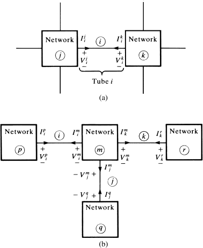
FIGURE 13.7 Definitions of the tube voltages and currents for (a) an individual tube and (b) and interconnection network.

The total number of equations in (13.7) equals the number of conductors incident at the termination/interconnection network (node). For the example of Figure 13.2 at interconnection network #4, this is 4 + 2 + 2 = 8. The equations in (13.7) are organized in the order of tube #1, then tube #2, and then tube #3. Within each row, the conductors of that tube are ordered sequentially according to their number. Each row refers to the conductor of the tube attached to the network. For example, the third row of (13.7) is for conductor 3 of tube #1, whereas the sixth row is for conductor #2 of tube #2 and the seventh row is for conductor #1 of tube #3. For a termination network such as the pth termination network in Figure 13.7, the representation is

The fact that this representation is completely general can be proven from the fact that it can be derived from a chain-parameter representation of the ports of the net-work, which always exits for any linear network. The representation in (13.7) has the sole purpose of enforcing (1) Kirchhoff's voltage law (KVL), (2) Kirchhoff's current law (KCL), and (3) the element relations that are imposed by the particular interconnections within the interconnection network. Each row of (13.7) represents a specific KVL constraint or a KCL constraint and/or an element relation for the termination/interconnection network for which (13.7) is being written. All of the entries in that row are zero with the exception of the following. Figure 13.8 illustrates some common examples. Figure 13.8(a) illustrates the kth conductor of the ith tube terminating in an open circuit within the mth network. The constraint here is that the current is zero:

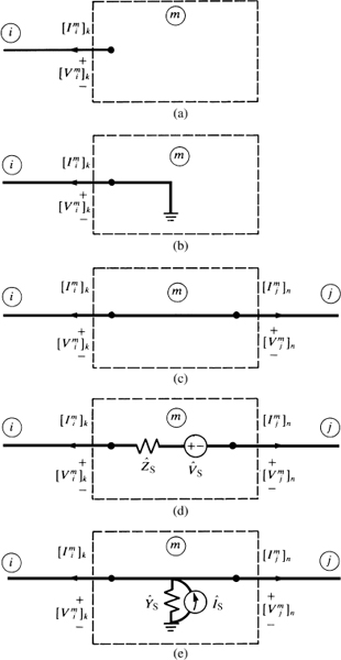
FIGURE 13.8 Illustration of the determination of the network characterizations for (a) an open circuit, (b) a short circuit, (c) a direct connection, (d) a Thevenin equivalent, and (e) a Norton equivalent.

Therefore, a 1 appears in the column of corresponding to the current of that conductor (the kth conductor) of that tube in and all other entries in that row of (13.7) are zero. Figure 13.8(b) illustrates the kth conductor of the ith tube terminating in a short circuit within the mth network. The constraint here is that the voltage is zero:

Therefore, a 1 appears in the column of corresponding to the voltage of that conductor of that tube in and all other entries in that row of (13.7) are zero. Figure 13.8(c) illustrates a direct connection between the kth conductor of tube i and the nth conductor of tube j within the mth network. The constraints here are that the voltage of the conductor of the ith tube and the voltage of the conductor of the jth tube are equal and the sum of the currents of the conductor of the ith tube and the conductor of the jth tube equals zero:

The first constraint is imposed by placing a 1 in the column of corresponding to the voltage of that conductor of that tube in and by placing a −1 in the column of corresponding to the voltage of that conductor of that tube in , and all other entries in that row of (13.7) are zero. The second constraint is imposed by placing a 1 in the column of corresponding to the current of that conductor of that tube in and by placing a 1 in the column of corresponding to the voltage of that conductor of that tube in , and all other entries in that row of (13.7) are zero. Multiple connections of conductors can similarly be handled. For example, consider the case of three conductors, k of tube i, n of tube j, and p of tube l, connected at a common point within the network. KCL requires that the sum of the currents at that interconnection equals zero:

Similarly, KVL requires that the differences of two of the three pairs of the voltages that are interconnected equal zero:

Figure 13.8(d) illustrates a series connection of an impedance and a lumped voltage source. The constraints are that the currents are equal and the voltages are related by the element relations:

The first constraint is imposed by placing a 1 in the column of corresponding to the current of that conductor of that tube in and by placing a 1 in the column of corresponding to the voltage of that conductor of that tube in , and all other entries in that row of (13.7) are zero. The second constraint is imposed by placing a 1 in the column of corresponding to the voltage of that conductor of that tube in , placing a −1 in the column of corresponding to the voltage of that conductor of that tube in , placing in the column of corresponding to the current of that conductor of that tube in , and placing in in the row corresponding to the equation being written, and all other entries in that row of (13.7) are zero. Figure 13.8(e) illustrates a parallel connection of an admittance and a lumped current source. The constraints are that the voltages are equal and the currents are related by the element relations:

The first constraint is imposed by placing a 1 in the column of corresponding to the voltage of that conductor of that tube in and by placing a −1 in the column of corresponding to the voltage of that conductor of that tube in , and all other entries in that row of (13.7) are zero. The second constraint is imposed by placing a 1 in the column of corresponding to the current of that conductor of that tube in , placing a 1 in the column of corresponding to the current of that conductor of that tube in , placing in the column of corresponding to the voltage of that conductor of that tube in , and placing Î_S in in the row corresponding to the equation being written, and all other entries in that row of (13.7) are zero.

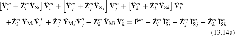
The final element of the process is the combination of the admittance parameters of the tubes and the constraint relations imposed by the termination/interconnection networks. The objective here is to write these termination/interconnection constraints as a set of simultaneous (complex) equations in terms of only the voltages at the ends of the tubes that are also the voltages at the ports of the termination/interconnection networks. Hence, we wish to solve for the termination voltages (versus frequency). A simple example will illustrate that result. Consider the mth network interconnecting tubes i, j, and k as shown in Figure 13.7(b), where the ith tube connects to termination network p at the other end, the jth tube connects to termination network q at the other end, and the kth tube connects to termination network r at the other end. The tube admittance characterizations at the mth end are

The network characterization is given for the mth interconnection network in (13.7a). Substituting (13.13) into (13.7) gives

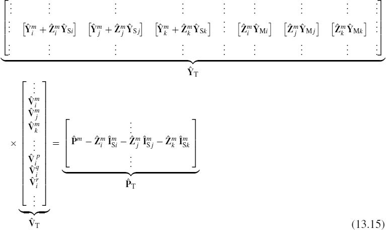
Similarly, for a termination network such as the pth termination network whose terminal characterization is given in Figure 13.7(b), the result is

This provides a simple rule for constructing the overall admittance matrix that can be solved for the voltages at the ends of each tube:

As an example, consider the transmission-line network in Figure 13.2 with graph shown in Figure 13.1(b). The admittance matrix becomes

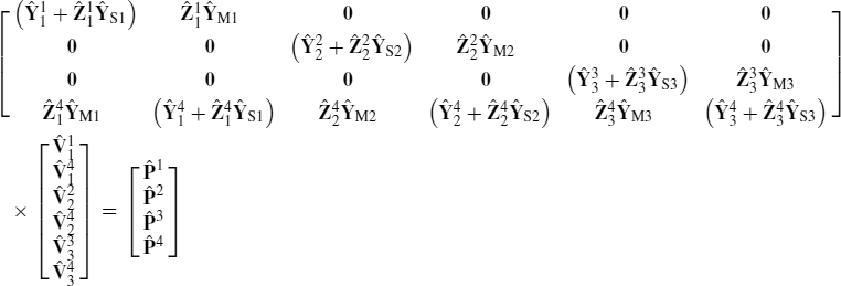
Numbering each conductor of each tube as shown gives the following. First, we examine termination network #1. The constraints are

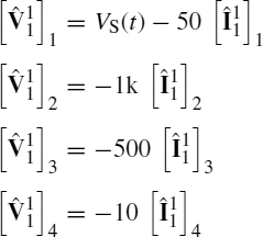
Therefore,

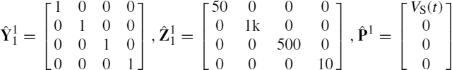
The number of equations equals the number of conductors incident on this node: 4. Similarly, termination networks #2 and #3 are characterized by

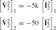
and

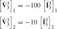
Hence, the termination network characterizations in (13.7b) become

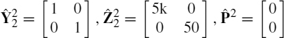
and

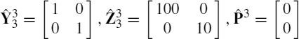
The number of equations equals the number of conductors incident on each node: 2. Interconnection network #4 has the following constraints. KVL imposes

KCL imposes

Observe that the total number of constraint equations for network #4 equals the total number of conductors incident on that node: 4 + 2 + 2 = 8. This requirement must always be met for any set of constraint equations for a termination/interconnection network. The interconnection network characterizations in (13.7a) become

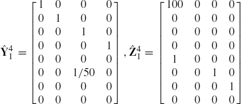
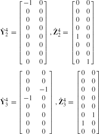
and

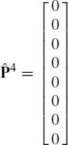
The predictions of this model with and without losses are compared for a pulse rise time of 1 ns in Figure 13.9. The predictions of the TDFD transformation are obtained by first determining the frequency-domain transfer function with this model at the spectral harmonics of the input using the above method. The resulting spectral components of the output voltage are combined using TIMEFREQ.FOR giving V_out(t). The predictions of the SPICE model in Figure 13.5 and those for this admittance parameter characterization using the TDFD conversion to the time domain for a lossless line are identical. The ramp waveform of Figure 13.3(c) is modeled as a trapezoidal waveform with identical τ_r = 1 ns rise and fall times and a 1-MHz repetition rate. This is decomposed into its spectral components and combined with the frequency-domain transfer function computed with the above admittance parameter model at 1000 harmonics. The bandwidth of this pulse is on the order of BW = 1/τ_r = 1 GHz. Hence, the excellent correlation with the SPICE results are expected. The frequency-dependent losses of the conductors were also included in the transfer function and the results recomputed and shown in Figure 13.9 using 1000 harmonics. The wire losses have a minor effect on the output voltage waveshape, which is probably due to the fact that the common ground plane losses are omitted. Figure 13.10 shows the frequency response of the transfer function obtained with this method with and without losses. This further confirms that the wire losses have little effect in this problem.

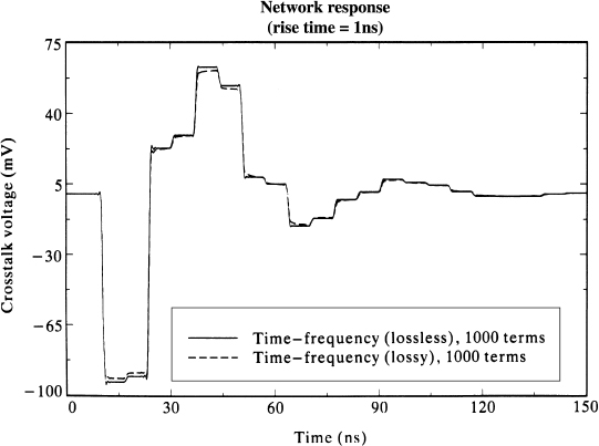
FIGURE 13.9 Comparison of crosstalk voltage at the termination of conductor #1 of tube #3 for the transmission-line network of Figure 13.2 for a rise time of 1 ns using the time-domain to frequency-domain transformation with and without losses.

The admittance parameters are not, of course, the only way of characterizing the tubes. The dual is the impedance parameter characterization:

The chain parameters in (13.1) can be manipulated to yield

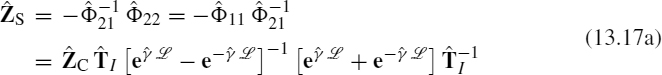
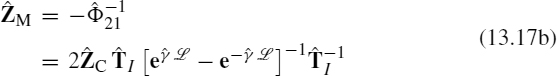
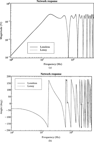
FIGURE 13.10 The frequency-domain crosstalk voltage at the termination of conductor #1 of tube #3 for the transmission-line network of Figure 13.2 with and without losses: (a) magnitude and (b) phase.

The overall matrix to be solved can be obtained by substituting (13.16) for the tubes connected to node m that is characterized by (13.7) to give

This result has the same form as (13.14) and (13.15) with the following substitutions:

With the impedance parameters we solve for the currents incident on the nodes, .

13.4 REPRESENTATION WITH THE BLT EQUATIONS

An alternative to the above methods is the use of the scattering parameter representation of the tubes [1,2,3]. Consider a tube having lumped excitation at some point, z = τ, along its length illustrated in Figure 13.11. These lumped excitations may represent point sources such as the direct attachment of a lightning stroke or can be extended to include distributed incident field excitation, as we will show. The general frequency-domain solution of the MTL (multiconductor transmission line) equations for this tube can be written as in Chapter 7 for the tube segments to the left and right of the sources as

FIGURE 13.11 Determination of the scattering parameters for a tube having lumped excitation at a point on the tube.

for 0 ≤ z < τ and

for τ < z ≤ . The subscripts on the undetermined constant vectors, L and R, represent the left and right segments, respectively. The characteristic impedance matrix is the inverse of the characteristic admittance matrix given in (13.5), and the propagation matrix is determined as in (13.4). Evaluating these at z = τ yields

Adding and subtracting these yields

The currents at the line endpoints can be logically decomposed into incident and reflected waves by evaluating (13.20b) at z = 0 and (13.21b) at z = as

where

where superscripts i and r denote incident and reflected, respectively. This is a sensible designation if we designate the incident wave as the portion incoming at the termination and the reflected wave as the portion outgoing from the junction and also observe that a component containing is traveling to the right and a component containing is traveling to the left. To conform with the results of the previous section, the tube currents are directed into the tube at both ends. Combining (13.23) and (13.25) yields the reflected components in terms of the incident quantities as

(There are sign differences between these results and those of [1–3] due to our choice of the total currents as being directed into the tube at both ends.) In matrix notation, these become

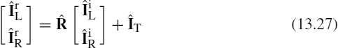
where the tube propagation matrix is

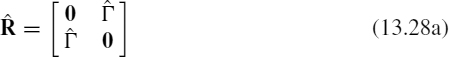
with entries

The current source vector due to the lumped sources at z = τ is

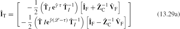
In the case of distributed excitation such as the case for incident field illumination of the tube, the source vector simply becomes

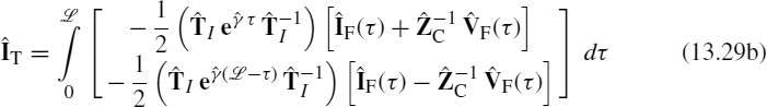
The total voltages and currents at the left end of the tube become, by evaluating (13.20) at z = and substituting (13.25a) and (13.25b),

Similarly, the total voltages and currents at the right end of the tube become, by evaluating (13.21) at z = and substituting (13.25c) and (13.25d),

Observe that, as in the case of the admittance parameters, the total currents are defined as being directed into the tubes at both ends. The incident components are defined as being the components traveling out of the tubes or into the network attached to that end. The reflected components are similarly defined as being the components traveling into the tubes or out of the network attached to that end. Hence, the origin of the names incident and reflected, with respect to the network or node at which the end of the tube is incident.

These results can be derived in an alternative manner from the chain-parameter matrix representation of the line with incident field illumination. Substituting the chain-parameter matrix of the line given in (12.25) of Chapter 12 into (13.30) and (13.31), we obtain (13.26). This gives the current source vector in (13.29b) in terms of the total incident field vectors, Î_FT and , developed in Chapter 12 and given in (12.25) as

We next form the junction scattering matrix for node m, , which relates the reflected and incident current components at node m as

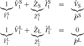
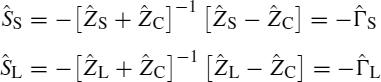
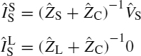
The number of equations here equals the total number of conductors incident on that node. First, consider a termination node where only one tube is incident as shown in Figure 13.12. Suppose that the network contains no lumped sources and is characterized by a generalized Thevenin equivalent as

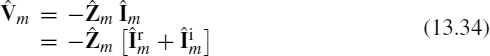
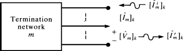
FIGURE 13.12 Definitions of incident and scattered waves for determining the scattering parameters of a termination network.

(Recall that the total currents are defined as being directed into the tube ends and are therefore directed out of the termination networks.) The relations for the voltage and current at the end of the tube that is incident on this node are

Solving (13.34) and (13.35) yields the current scattering matrix:

This has a direct parallel to the scalar current reflection coefficient for a two-conductor line [A.1].

The next form of the scattering matrix is for an interconnection network wherein there are two or more tubes incident. In the admittance parameter representation of the previous section, we characterized these in a general sense as a combination of generalized Thevenin and generalized Norton equivalents so that series and parallel impedances and excitation sources could be included. The formulation of the BLT equations in [1–3] has the excitation sources as lumped or distributed sources along the tubes due to incident fields. We will derive the BLT equations with that assumption although we will later modify them for the more general case of lumped sources within the networks. Thus, the interconnection networks will simply have (1) conductors directly connected, (2) conductors terminated in short circuits, and (3) conductors terminated in open circuits as shown in Figure 13.13. First consider the direction connection of several conductors as shown in Figure 13.13(a). This is characterized as

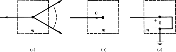
FIGURE 13.13 Interconnection networks: (a) direct connection, (b) open circuit, and (c) short circuit.

where Î_m contains the total currents of the conductors incident on the mth node and contains the voltages of those conductors. The first relation in (13.37a) enforces KCL at the connection so that for each connection a 1 appears in the columns of C_I corresponding to the currents of Î_m for the conductors that are connected. The second condition in (13.37b) enforces KVL at the connection so that for n conductors connected, there are n−1 equations enforcing for n−1 pairs of the voltages. Thus, a 1 appears in the column of C_V corresponding to the voltage of the pair in and a −1 appears in the column of C_V corresponding to the other voltage of the pair in . The second situation is an open circuit as illustrated in Figure 13.13(b). Enforcing KCL requires that we place a 1 in the column of C_I corresponding to the current of Î_m that is constrained to zero by the open circuit. The third constraint is a short circuit illustrated in Figure 13.13(c). Enforcing KVL requires that we place a 1 in the column of C_V corresponding to the voltage of that is constrained to zero by the short circuit. The sum of the row dimensions of C_I and C_V must equal the total number of conductors incident on the node. The scattering matrix for this interconnection node can now be formulated. Decomposing the total currents and voltages into their incident and reflected components gives

where contains the characteristic impedance matrices of the tubes incident on the node on the main diagonal and zeros elsewhere. Solving (13.38) yields the scattering matrix of the interconnection node as

Arranging the tube characterizations for all tubes in the network and the scattering matrix representations for all nodes in the network yields the overall characterization

The overall tube propagation matrix is 2n_T × 2n_T, where n_T is the total number of conductors in the overall transmission-line network and has the individual tube characterization matrices given in (13.27) on the main diagonal and zeros elsewhere. Similarly, the overall junction scattering matrix is 2n_T × 2n_T and contains the individual scattering matrices for the interconnection and termination networks on the main diagonal and zeros elsewhere. Combining (13.40) gives

which are referred to as the BLT (Baum, Liu, and Tesche) equations. The total currents can be obtained by writing

Solving (13.40) and (13.42) simultaneously gives the total currents as

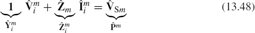
This formulation can be extended to include series and parallel impedances and lumped sources in the termination/interconnection networks. In order to provide that extension, consider the general characterization of the mth termination/interconnection node illustrated in Figure 13.7(b) and given in (13.7a):

This can be written in matrix form as

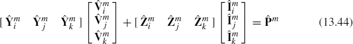
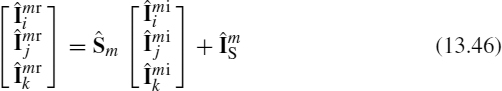
The currents and voltages can be decomposed into incident and reflected components according to (13.31) as

and likewise for tube j and tube k. Substituting (13.45) into (13.44) yields

where

and the collection of characteristic impedance matrices of the tubes incident on the termination/interconnection network is

The current source vector is

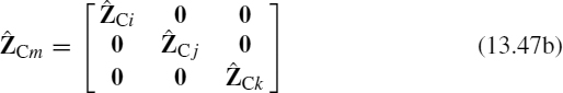
For example, consider the case of a termination network (only one tube incident on the node) and a generalized Thevenin representation of this network:

The above representation becomes

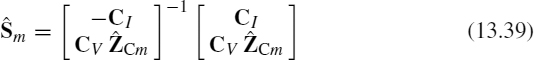
Thus, the scattering parameter representation in (13.33) has been modified to include lumped sources in the termination/interconnection networks. In the case of an interconnection network containing only short circuits, open circuits, and/or direct connections, this representation becomes

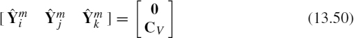
and

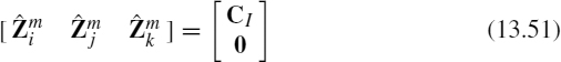
where C_V and C_I were originally defined in (13.37). Substituting (13.50) and (13.51) into (13.47a) yields (13.39).

The tube characterizations in (13.27) remain unchanged. Thus, the overall representation of the network is of the form in (13.40):

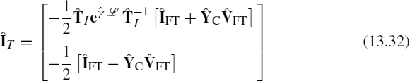
where is 2n_T × 2n_T and contains the individual scattering matrices given in (13.47a) on the main diagonal and zeros elsewhere, and Î_ST is 2n_T × 1 and contains the in (13.47c). In a fashion similar to the earlier derivation, we obtain the general form of the BLT equations for the total tube currents as

For example, consider the two-conductor line shown in Figure 6.1 of Chapter 6 (without incident field illumination). The total tube propagation matrix is simply (13.28) since there is only one tube and becomes

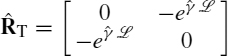
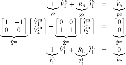
Writing (13.44) at the source and at the load gives

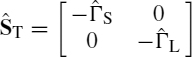
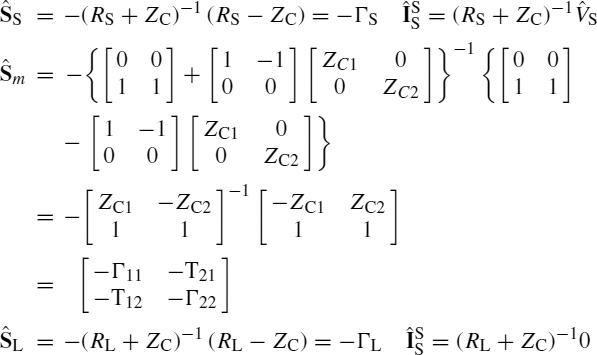
Thus, the scattering matrices at the source and the load in (13.47a) become

where and are the voltage reflection coefficients at the source and the load, respectively. The current reflection coefficients are the negatives of these [A.1]. Thus, the overall scattering matrix is

Also, the current source vectors in (13.47c) become

so that the overall current source vector becomes

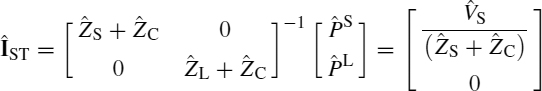
Forming the BLT equation in (13.53) for the total currents yields

Recalling that and , these results are identical to those derived in Chapter 6 and given in Eqs. (6.40b) and (6.41b).

The time-domain solution can be obtained from this formulation by first using the BLT equations to obtain the frequency-domain transfer function and then using the TDFD transformation method as before. Again, that technique for obtaining the time-domain solution assumes linear loads and tubes since superposition is implicitly used.

13.5 DIRECT TIME-DOMAIN SOLUTIONS IN TERMS OF TRAVELING WAVES

With the exception of the SPICE solution method, the above solution methods concentrated on the frequency-domain solution of transmission-line networks. The time-domain solution can be obtained from this solution via the TDFD technique, which is very straightforward and has been used on numerous occasions. Of course, the TDFD technique requires linear terminations. In this final section, we briefly investigate the direct time-domain solution via the traveling waves existing on the various tubes of the network.

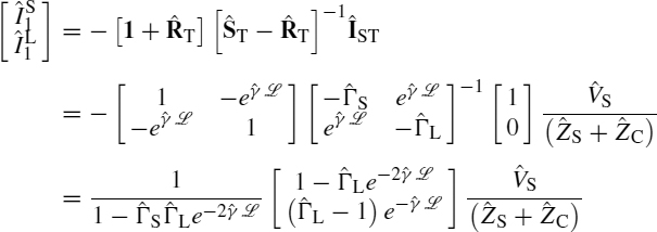
To begin the discussion, consider a tandem connection of two-conductor lines having a discontinuity as shown in Figure 13.14(a). Each line is characterized by a characteristic impedance Z_Ci and time delay T_Di. Lossless lines and resistive terminations are assumed to simplify the discussion. The frequency-domain solutions on each line are of the form

in accordance with the general solution of the transmission-line equations for each tube. The discontinuity may be characterized as before with a form of voltage scattering parameter matrix that relates the incident and reflected voltage waves at that point as illustrated in Figure 13.14(b). The incident waves are the portions of (13.45a) that are incoming at the junction, and . The reflected waves are the portions of (13.54a) that are outgoing at the junction, and . Hence we may write

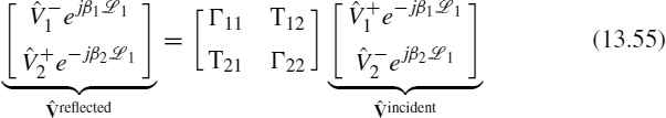
FIGURE 13.14 Determination of the scattering parameters at the junction of two different two-conductor lines: (a) line configuration and (b) definition of incident and reflected voltage waves at the junction.

The Γ_ii elements are the voltage reflection coefficients and the T_ij elements are the voltage transmission coefficients. Figure 13.15 illustrates the determination of these parameters for various discontinuities. Consider the direct connection shown in Figure 13.15(a). The voltages and currents must be continuous. Equating Eqs. (13.54) for the left and right sections and putting them in the form of (13.55) yields

This result is directly analogous to the case of a uniform plane wave incident at an interface between two media [A.1]. It is a sensible result for the following reason. In the time domain, the wave incident from line #1 “sees” an impedance at the junction equal to the characteristic impedance of line #2 since it has not arrived at the termination of line #2 and therefore line #2 appears infinite in length. So the reflection coefficient can be calculated as though line #1 is terminated in the characteristic impedance of line #2. The transmission coefficient is easily calculated from the reflection coefficients since the total voltage incident on the junction from line #1 is the sum of the incident and reflected waves on that line that, because of the direct connection, must equal the transmitted voltage or (1 + Γ₁₁) = T₂₁. In a similar fashion, (1 + Γ₂₂) = T₁₂.

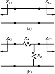
FIGURE 13.15 Illustration of the simplified determination of the scattering parameters for (a) a direct connection and (b) a resistive interconnection network.

The BLT equations can be easily formed for this network although their solution is best suited to computer implementation. The overall tube propagation matrix is

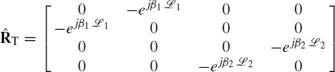
Writing (13.7) at the source, the junction, and the load gives

where m designates the “middle node” (the junction). The junction scattering matrices are obtained from (13.47a) as

Thus, the overall scattering matrix becomes

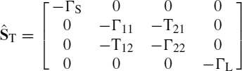
These reflection and transmission coefficients are the negative of the voltage reflection and transmission coefficients in (13.56) because we are considering currents and because of the current directions at the junctions (into the tubes). Additionally, the current transmission coefficients are and 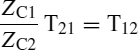in the same fashion as uniform plane waves [A.1]. The total current source vector is

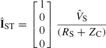
The BLT equations are then formed from (13.53) with Î_TT = 0 (no incident field illumination).

Figure 13.15(b) shows a connection consisting of a resistive network. For the above reasons, we may similarly determine

where

Determination of these is very similar to the case of plane waves normally incident on a boundary [A.1]. The notation denotes the parallel combination of two resistances as .

In the time domain, the source initially “sees” a termination of Z_C1 so that the voltage wave sent out is, by voltage division,

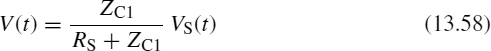
This wave travels down line #1 reaching the discontinuity at one time delay of T_D1, where Γ₁₁V(t − T_D1) is reflected and T₂₁V(t − T_D1) is transmitted across the junction. The reflected portion arrives at the source at 2T_D1 where a portion of it, Γ_SΓ₁₁V(t − 2T_D1), is sent back toward the junction where a portion of it is reflected, Γ₁₁Γ_SΓ₁₁V(t − 3T_D1), and a portion is transmitted, T₂₁Γ_SΓ₁₁V(t − 3T_D1), and so on. Meanwhile, the portion of the original wave that was transmitted across the junction, T₂₁V(t − T_D1), arrives at the load where it is reflected as Γ_LT₂₁V(t − T_D1 − T_D2). This is sent back to the junction where a portion of it, Γ₂₂Γ_LT₂₁V(t − T_D1 − 2T_D2), is reflected back toward the load and a portion, T₁₂Γ_LT₂₁V(t − T_D1 − 2T_D2), is transmitted across the junction onto line #1. This process of continued reflections and transmissions continues, and the total voltage at any point on either line is the sum of the total waves at that point and time. Clearly, the line voltages will be linear combinations of the initial transmitted wave, V(t), delayed in time by various sums of multiples of the line delays T_D1 and T_D2. A lattice diagram can be constructed as described in Chapter 6 to aid in determining these total voltages but the process is clearly very complicated owing to the multitude of reflections and transmissions. If either line is terminated in its characteristic impedance, the summation is simplified considerably, and a series solution can be developed [A.3]. But for completely mismatched lines, the summation is tedious.

A symbolic solution can be obtained if we use the time-shift or difference operator as before:

in the BLT equations of (13.53). Thus,

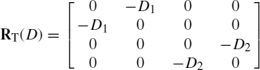
The BLT equations in (13.53) with Î_TT = 0 (no incident field illumination) can be written as

and [R_T(D) + 1]⁻¹ is simple to obtain. However, the literal solution of the BLT equations is very tedious even for this simple case. If we substitute a previously described SPICE model for each line, the summation of these waves is taken care of and nonresistive loads can be considered. A direct time-domain summation of the traveling waves was implemented using the scattering parameters of the termination/interconnection networks in [3] but, once again, keeping track of all the incident/reflected waves on the line is a very tedious task because of the multiple reflections/transmissions and the different mode velocities on each tube.

13.6 A SUMMARY OF METHODS FOR ANALYZING MULTICONDUCTOR TRANSMISSION LINES

If one is willing to forego losses, then the simplest and most accurate solution method for transmission-line networks is to use SPICEMTL.FOR or SPICEINC.FOR to build SPICE subcircuit models for the tubes and then imbed them in an overall SPICE circuit model where the termination networks as well as the interconnection networks are attached. This method is extraordinarily simple to implement and, in addition, it will handle nonlinear terminations such as diodes, transistors, and so on in the termination/interconnection networks. The author strongly recommends this method of analyzing lossless transmission-line networks. Including losses of the tubes is the only challenging problem left. However, the admittance parameter method can be used to incorporate losses and the TDFD method can be used to return to the time domain. The only disadvantage of this method is that the termination/interconnection networks must be linear, since superposition is used to return to the time domain. In addition, the FDTD method using a state-variable characterization of the termination/interconnection networks can handle transmission-line networks that have losses as well as nonlinear terminations [B.27, B.29].

These remarks also apply to single tube networks that we studied for the first 12 chapters of this text. This long journey in the study of methods for analyzing MTLs can therefore be summarized as follows. For lossless lines, the solution process is virtually trivial: generate SPICE/PSPICE subcircuit models with SPICEMTL.FOR or SPICEINC.FOR and then imbed these into an overall SPICE program where the terminations are attached. If losses of the lines (conductor and/or dielectric) must be included in the analysis, then we have a choice of several methods: (1) The time-domain to frequency-domain (TDFD) method where losses are included in the frequency-domain transfer function at the harmonics of the input source, (2) the finite-difference, time-domain (FDTD) method where losses are included in the numerical evaluation of the convolution integral via the Prony method, for example, or (3) for electrically short lines, modeling the line with a lumped-Pi or lumped-T equivalent circuit but the losses must be frequency-independent. The lumped-Pi and lumped-T approximate circuit models require that the per-unit-length resistances and internal inductances of the conductors be their dc values and the conductance must be frequency independent since frequency-dependent elements are not readily modelable directly in the time domain in lumped circuit models. There are, however, some equivalent circuits that tend to mimic frequency-dependent behavior of these elements to some degree. (See Figure 8.50).

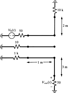
FIGURE P13.11

PROBLEMS

• 13.1 Derive the admittance parameters given in (13.3).
• 13.2 Derive the admittance parameter relation for a transmission-line network given in (13.15) and for the problem in Figure 13.2.
• 13.3 Derive the impedance parameters given in (13.17).
• 13.4 Derive the relations given in (13.26) and (13.27).
• 13.5 Derive the scattering parameter relation for a termination network given in (13.36).
• 13.6 Derive the scattering parameter relation for an interconnection network given in (13.39).
• 13.7 Derive the BLT equations given in (13.41) and in (13.43).
• 13.8 Derive the scattering parameter matrix and current source vector given for the general case in (13.47).
• 13.9 Derive the BLT equations for the general case given in (13.53).
• 13.10 For the tandem connection of two-conductor lines shown in Figure 13.14, derive series expressions for the time-domain source and load voltages in terms of delayed source voltage waveforms for a matched load on line #2, that is, R_L = Z_C2.
• 13.11 Consider the transmission-line network shown in Figure P13.11. All conductors are #20 gauge wires (r_w = 16 mils) at a height of 1 cm above a ground plane. Solve for the voltage V_out(t) where V_S(t) is a 10-MHz trapezoidal pulse train with rise/fall times of 1 ns and 50% duty cycle. compute this using (a) the SPIcE model, (b) the lumped-Pi model, (c) the admittance parameter model, (d) the impedance parameter model, and (e) the BLT equations.

REFERENCES

[1] C. E. Baum, T. K. Liu, F. M. Tesche, and S. K. chang, Numerical results for multiconductor transmission-line networks, Interaction Note 322, Air Force Weapons Laboratory, Albuquerque, NM, September 1977.

[2] C. E. Baum, T. K. Liu, and F. M. Tesche, On the analysis of general multiconductor transmission-line networks, Interaction Note 350, Air Force Weapons Laboratory, Albuquerque, NM, November 1978.

[3] A. K. Agrawal, H. K. Fowles, L. D. Scott, and S. H. Gurbaxani, Application of modal analysis to the transient response of multiconductor transmission lines with branches, IEEE Transactions on Electromagnetic Compatibility, 21(3), 256–262, 1979.

[4] c. R. Paul, Analysis of electromagnetic coupling in branched cables, Proceedings of the 1979 IEEE International Symposium on Electromagnetic Compatibility, San Diego, cA, August 1979.

[5] J. L. Allen, Time-domain analysis of lumped-distributed networks, IEEE Transactions on Microwave Theory and Techniques, 27(11), 890–896, 1979.

[6] F. M. Tesche and T. K. Liu, User manual and code description for QV7TA: a general multiconductor transmission-line analysis code, Interaction Application Memos, Memo 26, LuTech, Inc., August 1978.

[7] A. R. Djordjevic and T. K. Sarkar, Analysis of time response of lossy multiconductor transmission line networks, IEEE Transactions on Microwave Theory and Techniques, 35(10), 898–907, 1987.