
9
TIME-DOMAIN ANALYSIS OF MULTICONDUCTOR LINES
In the previous chapter, we examined the time-domain solution of the transmission-line equations and the incorporation of the terminal constraints for two-conductor lines. We will extend those results to the case of lines composed of more than two conductors or multiconductor transmission lines (MTLs) in this chapter. We will find that the results of the preceeding chapter for two-conductor lines can be extended to the case of MTLs consisting of n + 1 conductors with n > 1 in a very straightforward manner using matrix notation.
9.1 THE SOLUTION FOR LOSSLESS LINES
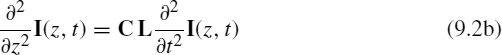
In this section, we will examine the time-domain solution of the MTL equations for a lossless line:
where L and C are the per-unit-length inductance and capacitance matrices, respectively, and are of dimension n × n. The line voltages and currents are contained in the n × 1 vectors V and I. The uncoupled, second-order equations are

Note that the order of multiplication of L and C in these second-order equations must be strictly observed. The objective in this section is to determine the general solution of these equations and the incorporation of the terminal conditions. Some earlier works are represented by [1–9].
9.1.1 The Recursive Solution for MTLs
In the previous chapter, we developed a series solution for the terminal voltages of a lossless, two-conductor line. (See Eq. (8.14) in the previous chapter.) Branin's method was also developed for two-conductor lossless lines and expressed the terminal voltages at one end of the line in terms of the terminal voltages at the other end one-time delay earlier. This led to the SPICE exact solution model for two-conductor, lossless lines. The series solution can be extended in the following manner to lossless MTLs in homogeneous media. The following recursive solution cannot be readily extended to handle inhomogeneous media. Recall the frequency-domain chain parameter matrix as

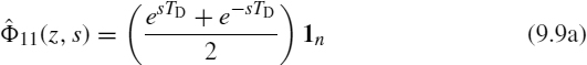
where the submatrices are given in (7.115) of Chapter 7. Specializing these for a lossless line in a homogeneous medium gives
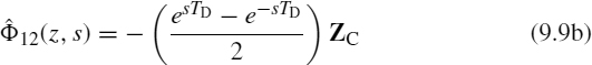
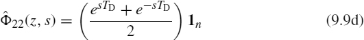
where 1n is the n × n identity matrix with ones on the main diagonal and zeros elsewhere. The n × n characteristic impedance matrix is defined as
and the velocity of propagation for this homogeneous medium is defined by

The phase constant in (9.4) is β = ω/v.
The Laplace transform of the corresponding time-domain result can be obtained from this by substituting the Laplace transform variable s for jω, and replacing
where the line one-way time delay is again denoted as
The Laplace-transformed chain parameter matrices in (9.4) become

Hence, taking the Laplace transform of the chain-parameter relation in (9.3) shows that the terminal voltages and currents are related as


Multiplying (9.10b) by ZC and adding and subtracting the equations gives
Observing once again the delay transform pair given in (8.43) of Chapter 8 gives the time-domain forms as
Time shifting (9.12b) and rearranging gives
Define the vectors
Equations (9.12) become
Equations (9.13) after being time shifted become
Substituting (9.14) into (9.15) gives the terminal voltages in terms of the E vectors as
In order to incorporate the terminal constraints at the ends of the line, we describe the resistive terminations as generalized Thevenin equivalents:
Substituting these terminal relations into (9.15) and (9.14) gives
where we have defined, in the fashion for two-conductor lines, the n × n reflection coefficient matrices as
and the n × n voltage division coefficient matrices are defined as
The scheme is to discretize the time axis into N computation steps in each oneway time delay TD as Δt = TD/N and then form the four n × N arrays ![]() ,
, ![]() ,
, ![]() , and
, and ![]() . The N columns of these are associated with the time increment, and the n rows are associated with the particular conductor of the line. To begin the recursion algorithm, we assume an initially relaxed line and fill
. The N columns of these are associated with the time increment, and the n rows are associated with the particular conductor of the line. To begin the recursion algorithm, we assume an initially relaxed line and fill ![]() and
and ![]() with zero entries. Then compute the entries in
with zero entries. Then compute the entries in ![]() and
and ![]() according to (9.18) and compute the terminal voltages from (9.16). Once all entries are filled for all N time increments for 0 ≤ t ≤ TD, write the entries in
according to (9.18) and compute the terminal voltages from (9.16). Once all entries are filled for all N time increments for 0 ≤ t ≤ TD, write the entries in ![]() and
and ![]() into
into ![]() and
and ![]() , respectively, and repeat the calculations for the N time increments in the next interval TD ≤ t ≤ 2TD. This is repeated to solve for the terminal voltages in blocks of time of length equal to the one-way line delay, TD. This extension of Branin's method to MTLs is implemented in the FORTRAN program BRANIN.FOR described in Appendix A. The method implicitly assumes that all modes propagate with the same velocity so that it does not appear feasible to extend it to the lines in inhomogeneous media.
, respectively, and repeat the calculations for the N time increments in the next interval TD ≤ t ≤ 2TD. This is repeated to solve for the terminal voltages in blocks of time of length equal to the one-way line delay, TD. This extension of Branin's method to MTLs is implemented in the FORTRAN program BRANIN.FOR described in Appendix A. The method implicitly assumes that all modes propagate with the same velocity so that it does not appear feasible to extend it to the lines in inhomogeneous media.
The recursive method can be solved in series form by recursively substituting (9.18) into (9.16) to give
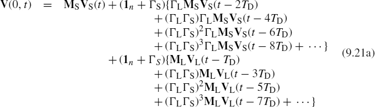
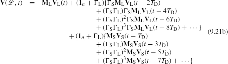
These reduce to the exact scalar results for a two-conductor line given in (8.14) of Chapter 8, but the order of multiplication of the matrices must be preserved here.
Equations (9.21) show that in order to eliminate reflections at the terminations, we must terminate the line in matched loads, that is, RL = ZC and/or RS = ZC, in which case (9.19) become ΓL = 0n and ΓS = 0n where 0n is the n × n zero matrix with zeros in all positions. Therefore, in order to “match” an MTL, we must provide resistors between all pairs of lines [1]. It is not sufficient to simply attach resistors between each line and the reference conductor to eliminate reflections, as was the case for two-conductor lines. If the line is matched at the right end, that is, RL = ZC, then ΓL = 0n and (9.21) become
and
and ML = 21n. Suppose that the sources are only in the left termination, that is, VL(t) = 0. These results reduce to
and
which simply says that the input voltages to the line are the “voltage-divided” portions of the sources in the left termination, VS(t), and the output voltages at the right end of the line are those delayed by one line one-way delay TD, which means that there are no reflections. The result in (9.21c) for the voltage at z = 0, V(0, t), is composed of two contributions. The source in the left termination, VS(t), produces (9.21e), and the source in the right termination, VL(t), is “voltage-divided” by ML, sent down to the source arriving there after one-time delay, reflected by ΓS, added to the incident wave, and sent back down the line to the load where it is completely absorbed. Similarly, the result in (9.21d) for the voltage at z = ![]() , V(
, V(![]() , t), is composed of two contributions. The source in the left termination, VS(t), produces (9.21f), and the source in the right termination, VL(t), is “voltage-divided” by ML, sent down to the source, reflected by ΓS, and sent back down the line to the load arriving after two-time delays where it is completely absorbed.
, t), is composed of two contributions. The source in the left termination, VS(t), produces (9.21f), and the source in the right termination, VL(t), is “voltage-divided” by ML, sent down to the source, reflected by ΓS, and sent back down the line to the load arriving after two-time delays where it is completely absorbed.
9.1.2 Decoupling the MTL Equations
The primary technique used to determine the general form of the solution of the MTL equations for sinusoidal, steady-state excitation in Chapter 7 was to decouple them with similarity transformations. In the case of the general time-domain solution of lossless lines, the technique of decoupling the MTL equations in (9.1) or (9.2) via similarity transformations is again a useful technique that can always be used to affect the solution.
We define the similarity transformations to mode voltages and currents as
Substituting these into (9.1) gives

or for the uncoupled second-order equations in (9.2)


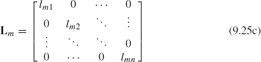
If we can choose a TV and a TI such that (9.23) or (9.24) are uncoupled, then we have the general form of the mode solutions as those of two-conductor lines of the previous chapter. This is always guaranteed for lossless lines as was shown in Chapter 7 for sinusoidal excitation. For example, consider the coupled first-order equations in (9.23). Suppose we can find a TV and a TI such that they simultaneously diagonalize both L and C as
where Lm and Cm are diagonal as

Then the mode equations in (9.23) become

or
These are the same equations as for uncoupled, two-conductor lines having characteristic impedances of

and velocities of propagation of

for i = 1, 2,…, n. Therefore, the solutions for these mode voltages and currents have the same general form as for the two-conductor line. The actual voltages and currents can be obtained from the forms of the mode voltages, and current solutions via (9.22). We now address the determination of the diagonalizing similarity transformation for the various classes of lines.
9.1.2.1 Lossless Lines in Homogeneous Media
For this class of line, we have the important identity
where the surrounding homogeneous medium is characterized by permittivity ε and permeability μ. The similarity transformations that simultaneously diagonalize L and C as in (9.25) can be found in the following manner as shown in Chapter 7. Because L is real and symmetric, a real, orthogonal transformation T can be found such that
where
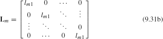
and the inverse of T is its transpose that is denoted with the superscript t [10]:
Similarly, with the aid of the identity in (9.30) expressed as
we may form
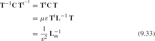
where ![]() . Comparing (9.31) and (9.33) to (9.25) shows that the transformations can be defined as
. Comparing (9.31) and (9.33) to (9.25) shows that the transformations can be defined as
Therefore, the mode characteristic impedances in (9.28) are
and all modes have the same velocity of propagation:
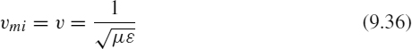
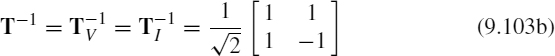
For the special case of a three-conductor line, n = 2, the mode transformation is simple [10]:
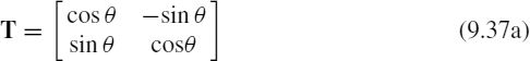
where

For n ≥ 3, a numerical computer subroutine implementing, for example, the Jacobi method is used to obtain the orthogonal transformation [10]. Appendix A describes a FORTRAN subroutine, JACOBI.SUB, that accomplishes this reduction.
9.1.2.2 Lossless Lines in Inhomogeneous Media
For this case we no longer have the identity in (9.30). However, we showed in Chapter 7 that because L and C are real, symmetric, and positive definite, we can find a transformation that simultaneously diagonalizes these matrices in the following manner. First, we find an orthogonal transformation that diagonalizes C as
where

Since C is positive definite, we can obtain the square root of θ2, θ, which is real and nonsingular and forms the product θUtLUθ. Since this is real and symmetric, we can diagonalize it with another orthogonal transformation as
where
and
Define the matrix T as
The columns of T can be normalized to a Euclidean length of unity as
where α is the n × n diagonal matrix with entries
The mode transformations in (9.22) that simultaneously diagonalize L and C as in (9.25) can then be defined as


Substituting (9.43) and (9.44) into (9.25) gives

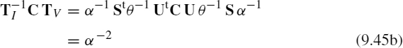
Comparing (9.45) and (9.25) shows that
Since α and Λ are diagonal matrices, the mode characteristic impedances and velocities of propagation are given by
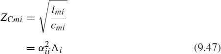
and

One can show that ![]() . The desired mode transformation matrices are
. The desired mode transformation matrices are
The above diagonalization is implemented in the FORTRAN subroutine DIAG.SUB described in Appendix A. This subroutine calls the FORTRAN subroutine JACOBI.SUB to compute the two orthogonal transformations required by DIAG.SUB.
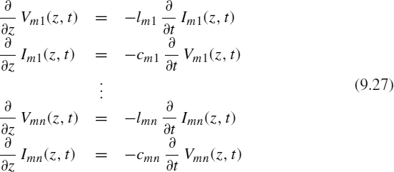
9.1.2.3 Incorporating the Terminal Conditions via the SPICE Program
Since we have uncoupled the equations via the mode transformation in the preceding sections, the mode voltages and currents are essentially associated with n uncoupled, two-conductor transmission lines as is illustrated in (9.27) whose general solutions are known. Again each general mode solution contains two undetermined constants so that there are a total of 2n undetermined constants. It remains to incorporate the terminal conditions at the two ends of the line in order to evaluate these 2n undetermined constants.
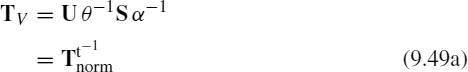
There are a number of ways of doing this. The most useful and simplest way is to utilize the exact time-domain model for a lossless, two-conductor line that exists in the SPICE code as shown in Figure 8.9 of Chapter 8 [A.2,A.3,B.19,11]. But each of these models relates only the n mode voltages and currents at the two ends of the line. In order to relate these mode quantities to the actual voltages and currents, we implement the mode transformations given in (9.22). These transformations can be implemented in the SPICE program through the use of controlled sources as illustrated in Figure 9.1. Writing the transformations in (9.22) out gives
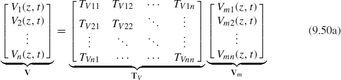
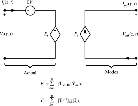
FIGURE 9.1 Illustration of the use of controlled sources to implement the mode transformations.
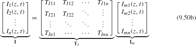
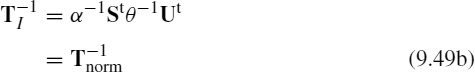
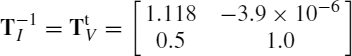
Inverting (9.50b) gives
Hence, the rows of (9.50c) and 9.50c can be written as
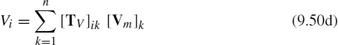
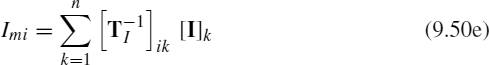
where we denote the entries in the ith row and jth column of TV and ![]() as [TV]ij and
as [TV]ij and ![]() , respectively, and the entries in the ith rows of the vectors Vm and I are denoted as [Vm]i and [I]i, respectively. The transformations in (9.50a) and (9.50c) can be implemented in SPICE using the controlled source representation illustrated in Figure 9.1. Zero-volt voltage sources are placed in each input to sample the current Ii(z, t) for use in the controlled sources representing the transformation in (9.50e). The interior two-conductor mode lines having characteristic impedance ZCmi and time delay TDi =
, respectively, and the entries in the ith rows of the vectors Vm and I are denoted as [Vm]i and [I]i, respectively. The transformations in (9.50a) and (9.50c) can be implemented in SPICE using the controlled source representation illustrated in Figure 9.1. Zero-volt voltage sources are placed in each input to sample the current Ii(z, t) for use in the controlled sources representing the transformation in (9.50e). The interior two-conductor mode lines having characteristic impedance ZCmi and time delay TDi = ![]() /vmi are simulated with the existing two-conductor SPICE model as
/vmi are simulated with the existing two-conductor SPICE model as
![]()
as shown in Figure 9.2.

FIGURE 9.2 The two-conductor mode transmission lines.
The advantages of this method of implementing the terminal conditions are that the model for the line is independent of the terminations and any of the available device models in SPICE such as resistors, capacitors, inductors as well as the nonlinear models such as diodes and transistors can be called. Hence, the model is referred to as a macromodel of the line and also called a 2n-port model of the line. The user need not redevelop the mathematical models of those devices in the terminations. The overall model of the line can be implemented as a subcircuit model in SPICE and the appropriate line terminations attached to the ports of this subcircuit. Thus, the solution implemented in this way in SPICE (or PSPICE) is exact within the time step discretization in the SPICE solution.
As an example of the implementation of this valuable technique, consider the example of three rectangular cross-section conductors (lands) on the surface of a printed circuit board (PCB) shown in Figure 9.3 that has been considered previously. This problem is that of an inhomogeneous medium, and we shall assume a lossless medium and perfect conductors so that the results of Section 9.1.2.2 will apply. The per-unit-length capacitance matrix was computed using the numerical technique described in Chapter 5 via the PCB.FOR program discussed in Appendix B using 50 divisions per land:

The per-unit-length inductance matrix was computed from the capacitance matrix with the dielectric board removed, C0, as
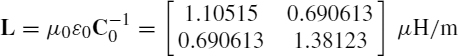
Using SPICEMTL.FOR, the similarity transformations become
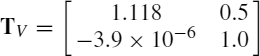
and
The mode characteristic impedances and propagation velocities are
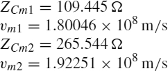
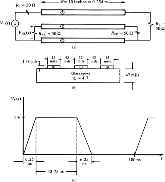
FIGURE 9.3 Example illustrating the generation of a SPICE model for coupled transmission lines: (a) longitudinal dimensions, (b) cross-sectional dimensions, and (c) the applied pulse train.
This gives the mode circuit one-way time delays as
![]()
The SPICE program (implemented on the personal computer version, PSPICE) is obtained from the circuit of Figure 9.4 as
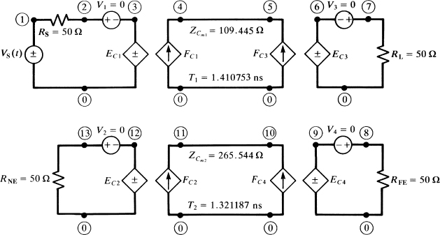
FIGURE 9.4 The SPICE model for the coupled line of Figure 9.3.
SPICE MTL MODEL
VS 1 0 PULSE(0 1 0 6.25N 6.25N 43.75N 100N)
RS 1 2 50
V1 2 3
RL 7 0 50
V3 7 6
RNE 13 0 50
V2 13 12
RFE 8 0 50
V4 8 9
EC1 3 0 POLY(2) (4,0) (11,0) 0 1.118 0.5
EC2 12 0 POLY(2) (4,0) (11,0) 0 -3.9E-6 1.0
EC3 6 0 POLY(2) (5,0) (10,0) 0 1.118 0.5
EC4 9 0 POLY(2) (5,0) (10,0) 0 -3.9E-6 1.0
FC1 0 4 POLY(2) V1 V2 0 1.118 -3.9E-6
FC2 0 11 POLY(2) V1 V2 0 0.5 1.0
FC3 0 5 POLY(2) V3 V4 0 1.118 -3.9E-6
FC4 0 10 POLY(2) V3 V4 0 0.5 1.0
T1 4 0 5 0 Z0=109.445 TD=1.410753N
T2 11 0 10 0 Z0=265.544 TD=1.321187N
.TRAN .1N 20N 0 .05N
.PRINT TRAN V(2) V(7) V(13) V(8)
.PROBE
.END
Comparisons with the experimentally obtained data will be shown in Section 9.3.2.
The method is implemented in the FORTRAN program SPICEMTL.FOR that is described in Appendix A. This code generates a SPICE subcircuit model. The user then imbeds this into a SPICE (PSPICE) program where the terminal constraints are added.
Another important advantage of the SPICE implementation of the solution is that the frequency-domain or sinusoidal steady-state phasor solution considered in Chapter 7 can also be obtained from this program with only a slight change in the control statements. These are to redefine the voltage source as
VS 1 0 AC 1
and redefine the control and print statements as
.AC DEC 50 10K 1000 MEG
(which solves the frequency-domain circuit from 10 kHz to 1 GHz in steps of 50 per decade) and
.PRINT AC VM(2) VP(2) VM(7) VP(7) VM(13) VP(13) VM(8) VP(8)
where VM(X) and VP(X) denote the magnitude and phase, respectively, of the voltage at node X. Adding the .PROBE statement to this allows the plotting of the frequency response in a decibel plot. The remaining statements in the original time-domain program above are unchanged.
9.1.3 Lumped-Circuit Approximate Characterizations
One can also model the line using a lumped-Pi or a lumped-T equivalent circuit so long as the line is electrically short at the highest significant frequency of the time-domain source waveform. These structures are shown for MTLs in Figure 7.6 of Chapter 7. For digital pulse waveforms having equal rise- and fall times τr, the highest significant frequency is approximately the bandwidth given earlier, fmax ![]() 1/τr. The line length is one tenth of a wavelength at this frequency if the pulse rise-/fall time is approximately 10 times the line one-way delay or
1/τr. The line length is one tenth of a wavelength at this frequency if the pulse rise-/fall time is approximately 10 times the line one-way delay or
τr > 10 TD
as was developed in Section 8.1.6.1 of Chapter 8. We saw that for MTLs there are n velocities of the modes. In order to determine whether the above criterion is satisfied, one should use the smaller of these mode velocities thereby guaranteeing that the condition will be satisfied at the larger mode velocities. However, in today's high-speed digital world, this criterion generally places impractically short-length limits on the PCB lands that can be modeled with one section. Other applications such as cables carrying signals with much lower spectral content perhaps can be feasibly modeled with lumped-Pi or lumped-T sections. Again, for higher spectral content signals, dividing the line into several sections that are individually short at the highest frequency of the pulse waveform has been shown to not significantly increase the model accuracy to justify the inordinately large circuit that must be solved [B.15]. For lossless lines, one is better off simply using the SPICE subcircuit model generated by SPICEMTL.FOR.
9.1.4 The Time-Domain to Frequency-Domain (TDFD) Transformation Method
This method is identical for MTLs to that described in Section 8.1.7 of Chapter 8 for two-conductor lines. The only slight difference is that one must compute the singleinput, single-output frequency-domain transfer function using a frequency-domain calculator such as MTL.FOR or using SPICEMTL.FOR to determine a MTL sub-circuit model, imbedding that generated model into a SPICE (PSPICE) program and using the .AC mode to compute this frequency-domain transfer function. Otherwise, there is no difference in its use for two-conductor lines or for MTLs. Once again, this method can incorporate line losses by including them in the frequency-domain transfer function (if MTL.FOR is used to generate it), which is a very straightforward process. However, the method suffers from the primary restriction that the line and its terminations must be linear since it uses the principle of superposition to return to the time domain.
9.1.5 The Finite-Difference, Time-Domain (FDTD) Method
The FDTD recursion relations were developed for a two-conductor line in the previous chapter. These are virtually unchanged for MTLs with only the use of matrix notation. Discretizing the derivatives in the MTL equations for a lossless line given in (9.1) using central differences [10,12] according to the scheme in Figure 8.17 gives

for k = 1, 2, ···, NDZ and

for k = 2, ···, NDZ. The n × 1 vectors I and V contain the line currents and line voltages, respectively, and we denote
Solving these gives the recursion relations for the interior points along the line as

for k = 1, 2, ···, NDZ and
for k = 2, 3, ···, NDZ.
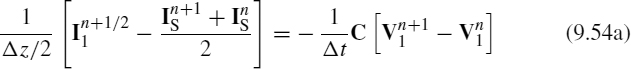
The second transmission-line equation given in Eq. (9.1b) is discretized at the source according to the scheme in Figure 8.18 as
Similarly, the second transmission-line equation, (9.1b), is discretized at the load according to the scheme in Figure 8.18 as

In these relations, we denote the n × 1 vectors of the currents at the source and at the load as IS and IL, respectively. Equations (9.54) are solved to give the recursion relations for the voltages at the source and the load:


It should be pointed out that this method of obtaining collocated current and voltage relations in (9.54) at the source and the load was shown in Chapter 8 to yield the exact solution of a two-conductor line consisting of perfect conductors immersed in a lossless, homogeneous medium for the magic time step of Δt = Δz/v.
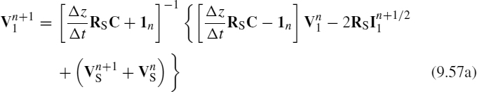
Assume that the multiconductor line has lumped terminal source and load representations that are resistive and are represented as generalized Thevenin equivalents:
Substituting these terminal representation of (9.56) into (9.55) yields the resulting FDTD recursion relations for the voltages at the source and at the load as
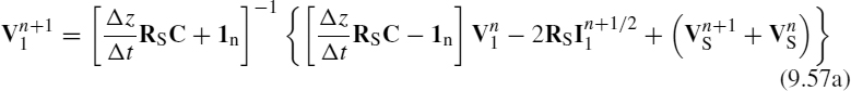
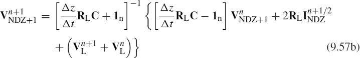
These equations are implemented in the FORTRAN program FINDIF.FOR described in Appendix A. Again the time step Δ t and the spatial discretization Δ z must satisfy the Courant condition

in order to guarantee stability of the solution. For MTLs in inhomogeneous media that have n velocities of propagation of the modes, the Courant condition should be satisfied by the larger of the mode velocities thereby guaranteeing that it will be satisfied by the smaller mode velocities.
9.1.5.1 Including Dynamic and/or Nonlinear Terminations in the FDTD Analysis
Any lumped-element network can be completely characterized in a state-variable form [13, 14]. In the case of a linear network, this completely general formulation becomes
with an associated output relation
The vector X contains the state variables of the lumped network. These are typically the inductor currents and capacitor voltages in that network or some subset of those variables. The vector U contains the independent sources in the network (the inputs), and the vector Y contains the designated outputs (currents and/or voltages) of the network. It should be emphasized that this formulation can characterize general linear networks that may contain such diverse conditions as inductor-current source cutsets and/or capacitor-voltage source loops as well as controlled sources of all types [13, 14].
Consider the recursion relations at the endpoints of the line given in (9.55a) and (9.55b). From these relations it is clear that we must configure the state-variable representations of the termination networks such that the outputs are the terminal currents IS and IL. The inputs for the state-variable representations must be the line voltages at the endpoints, V1 and VNDZ+1, as well as the independent sources within the termination networks. In order to accomplish this task, we will define the outputs in (9.59) as IS and IL and will partition the input vectors to yield
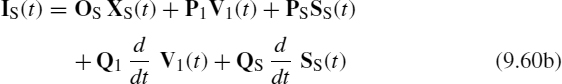
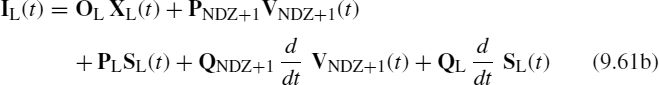
where subscripts S and L refer to the networks at the source and load ends, respectively. The independent sources within the termination networks are denoted as SS and SL. Observe that in this state-variable characterization of the termination networks, the terminal voltages V1 and VNDZ+1 are treated as being independent voltage sources driving the terminations.
We now address the problem of interfacing the state-variable characterizations of the termination networks with the recursion relations for the attached line. We need to discretize the state-variable forms in (9.60) and (9.61). We will choose the implicit backward Euler method (also called the first-order Adams–Moulton algorithm) [13]. This method is absolutely stable regardless of time step size so long as the termination network itself is stable: a necessary assumption [13]. Because of this, the Courant stability condition on Δt given in (9.58) must be enforced only on the solution for the MTL portion of the system. The state-variable forms in (9.60) for the source termination network are discretized using the backward Euler method to yield [B.24]

Solving (9.62a) for ![]() yields
yields
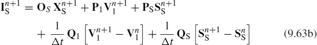
where 1 is the identity matrix with ones on the main diagonal and zeros elsewhere. Substituting (9.63b) into (9.55a) and combining with (9.63a) yields
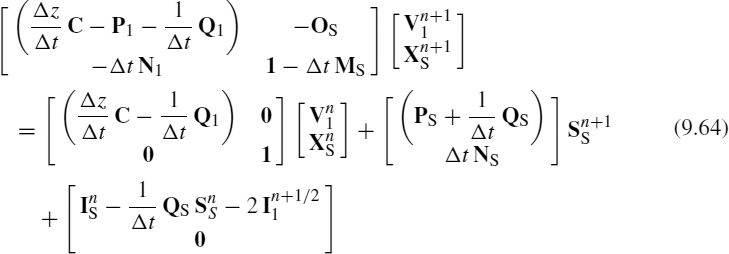
These simultaneous equations are solved for the new terminal voltages ![]() and state variables
and state variables ![]() . Vectors
. Vectors ![]() and
and ![]() contain the independent lumped sources in the termination network all of which are readily evaluated at the appropriate time steps. Vectors
contain the independent lumped sources in the termination network all of which are readily evaluated at the appropriate time steps. Vectors ![]() ,
, ![]() ,
, ![]() , and
, and ![]() are evaluated at the previous time step. Similarly, discretizing and combining (9.61) and (9.55b) yields the recursion relations for the load termination network as
are evaluated at the previous time step. Similarly, discretizing and combining (9.61) and (9.55b) yields the recursion relations for the load termination network as
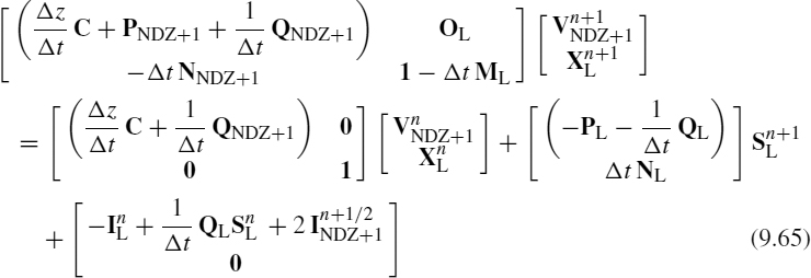
All variables in the right-hand side of (9.65) are known.
In the case of resistive terminations, the generalized Thevenin equivalent representation in (9.56) is written as
where ![]() and
and ![]() . Hence, XS = XL = 0 so that MS = N1 = NS = OS = Q1 = QS = 0 and ML = NNDZ+1 = NL = OL = QNDZ+1 = QL = 0 and P1 = −GS, PS = GS, PNDZ+1 = GL, PL = −GL. Equations (9.64) and (9.65) reduce to [B.24]
. Hence, XS = XL = 0 so that MS = N1 = NS = OS = Q1 = QS = 0 and ML = NNDZ+1 = NL = OL = QNDZ+1 = QL = 0 and P1 = −GS, PS = GS, PNDZ+1 = GL, PL = −GL. Equations (9.64) and (9.65) reduce to [B.24]

and
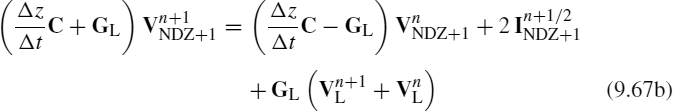
If we premultiply (9.67a) with ![]() and (9.67b) with
and (9.67b) with ![]() , these are identical to those derived earlier and given in (9.57) for this special case.
, these are identical to those derived earlier and given in (9.57) for this special case.
The solution sequence is as follows. First, write the state-variable descriptions of the terminations as given in (9.60) and (9.61). Equations (9.64) and (9.65) are then solved for the line voltages ![]() and
and ![]() and state variables of the termination networks
and state variables of the termination networks ![]() and
and ![]() . Next the line voltages
. Next the line voltages ![]() for k = 2, ···, NDZ are obtained from (9.53b). Finally, the currents are updated for k = 1, ···, NDZ via (9.53a). In order to insure stability of the solution for the lossless, single velocity case, the temporal and spatial discretizations should satisfy the Courant condition, which is Δt ≤ Δz/v, where v is the velocity of propagation in the medium. We will assume that the similar condition applies to the multimode, multivelocity MTL case where v is the maximum of the velocities of the modes along the line. The above method can be similarly implemented for the case of nonlinear termination networks [B.24].
for k = 2, ···, NDZ are obtained from (9.53b). Finally, the currents are updated for k = 1, ···, NDZ via (9.53a). In order to insure stability of the solution for the lossless, single velocity case, the temporal and spatial discretizations should satisfy the Courant condition, which is Δt ≤ Δz/v, where v is the velocity of propagation in the medium. We will assume that the similar condition applies to the multimode, multivelocity MTL case where v is the maximum of the velocities of the modes along the line. The above method can be similarly implemented for the case of nonlinear termination networks [B.24].
To compare the predictions of these models, we will investigate a three-conductor transmission line shown in Figure 9.5. Three conductors of rectangular cross section of width 5 mils and thickness 0.5 mils are separated by 5 mils and placed on one side of a silicon substrate having εr = 12 and thickness 5 mils as shown in Figure 9.5(b). The total line length is 50 cm and is terminated as shown in Figure 9.5(a). The source is a 1-V trapezoidal pulse having a rise/fall time of τr = τf = 100ps and pulse width of τ = 500 ps. The per-unit-length inductance and capacitance matrices are computed as
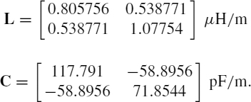
These give mode velocities in the lossless case of vm1 = 1.25809 × 10⁸m/s and vm2 = 1.47934 × 10⁸ m/s. The state-variable characterizations of the source and load given in (9.60) and (9.61) become
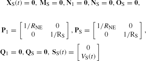
and
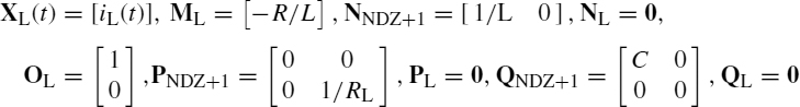
where C = 100 pF, L = 1 μH, R =10 Ω, RS = 50 Ω, RL = 50 Ω, and RNE = 5 Ω and iL(t) is the inductor current. Observe that the capacitor produces a voltage source-capacitor loop with [VNDZ+1]1. Hence, the coefficient of the derivative of VNDZ+1 in the terminal state-variable relation in (9.61b), QNDZ+1, is nonzero. We will compare the predictions of the SPICE (lossless) and the FDTD predictions. The FDTD spatial and temporal discretizations are denoted by

FIGURE 9.5 An example of a coupled line with dynamic loads: (a) longitudinal dimensions and loads, (b) cross-sectional dimensions, and (c) the applied pulse train.

Thus, the Courant stability criterion translates to
NDT ≥ NDZ × (final solution time) × v/![]() .
.
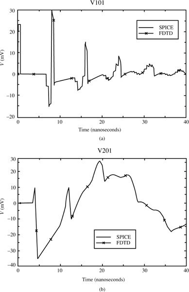
FIGURE 9.6 Predictions of the SPICE and FDTD models for the line of Figure 9.5: (a) V101 and (b) V201.
The bandwidth of the input pulse is on the order of 1/τr = 10 GHz. The spatial discretization for the FDTD results is chosen so that each cell is λ/10 using the smaller of the mode velocities vm1 at 20 GHz = 2 × 1/τr, giving NDZ = 795. At the Courant limit of Δt = Δz/v for this spatial discretization using the larger of the mode velocities vm2 and a total solution time of 40 ns, we obtain a total number of time points of NDT = 9410. Figure 9.6(a) and (b) show the predictions for voltages across the ends of the receptor line. The FDTD predictions are compared to the SPICE predictions and give identical results as they should.
9.2 INCORPORATION OF LOSSES
Losses arise from either the nonzero conductivity and polarization loss of the surrounding medium or from imperfect conductors. Of the two mechanisms, the loss introduced by imperfect conductors is usually more significant than the loss due to the medium for typical transmission line structures and frequencies up to around 10 GHz. The resistance due to imperfect conductors is represented in the n × n per-unit-length resistance matrix R. For lossy conductors, there is a n × n per-unit-length internal inductance matrix Li due to magnetic flux internal to the conductors. The frequency-dependent losses in the surrounding medium are contained in the n × n matrix G and can be represented with the Debye model as discussed in Section 8.2.1.1 in the previous chapter. This is fairly straightforward for a homogeneous surrounding medium. For a lossy, inhomogeneous medium, incorporating losses in this fashion becomes tedious.
In the frequency domain, the MTL equations can be written as


where L represents the external inductance, and the internal inductance is included in ![]() . To obtain the time-domain results we represent the MTL equations with the Laplace transform as
. To obtain the time-domain results we represent the MTL equations with the Laplace transform as


A common way of approximating the internal impedance term as discussed in the previous chapter is
This represents a reasonable approximation to the skin-effect behavior as can be seen if we substitute s = jω to yield

The n × n matrix A represents the dc per-unit-length resistance matrix. The n × n matrix ![]() represents the sum of the high-frequency per-unit-length resistance matrix and the high-frequency per-unit-length internal inductive reactance matrix. Hence, the entries in A and B are
represents the sum of the high-frequency per-unit-length resistance matrix and the high-frequency per-unit-length internal inductive reactance matrix. Hence, the entries in A and B are
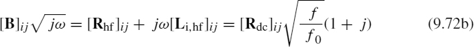
This assumes that the high-frequency resistance and internal inductive reactance of each conductor are equal. As we saw in Chapter 4, this is exact for isolated wires but is approximately true for conductors of rectangular cross section. This representation ignores the dc internal inductance of the conductors, which is typically dominated by the external inductance. The representation in (9.72b) also assumes that the break frequency f0, where the resistance and internal inductance transition from their dc behavior to their high-frequency ![]() behavior, is the same for all the conductors. This implicitly assumes that the conductors are identical. For example, an isolated wire transitions from its dc behavior to its high-frequency behavior when its radius equals two skin depths: rw = 2δ. If the conductors are not identical, this can be accommodated by putting the individual
behavior, is the same for all the conductors. This implicitly assumes that the conductors are identical. For example, an isolated wire transitions from its dc behavior to its high-frequency behavior when its radius equals two skin depths: rw = 2δ. If the conductors are not identical, this can be accommodated by putting the individual ![]() break frequencies into the individual B matrix terms giving the general representation in (9.71).
break frequencies into the individual B matrix terms giving the general representation in (9.71).
The Laplace transform representation in (9.69) translates in the time domain to
where * again denotes convolution, and the inverse Laplace transforms are denoted as
Using the Laplace transform identity given in the previous chapter:
the representation of the conductor internal impedance in (9.70) translates to

Hence, the convolution becomes

9.2.1 The Time-Domain to Frequency-Domain (TDFD) Method
This method of circumventing the convolution for lossy lines is essentially unchanged from previous descriptions except that the frequency-domain computation of the transfer function requires inclusion of the line losses. (See Section 8.2.2 of the previous chapter.) This is a very straightforward task and easily includes frequency-dependent losses. Simply compute the internal impedance at each frequency and include that in the solution for that frequency. Then recompute this for the next frequency and resolve for the transfer function (magnitude and phase) at that frequency and so on. The computer program MTL.FOR described in Appendix A provides this solution for lossy multiconductor lines, and the program TIMEFREQ.FOR recombines the processed Fourier frequency components of the time-domain input signal to indirectly give the time-domain response of the system. Once again, use of this method requires that the line terminations are linear since superposition was inherently used.
9.2.2 Lumped-Circuit Approximate Characterizations
Again, a common way of approximately representing the line is with a lumped-Pi or lumped-T equivalent circuit shown in Figure 7.6 of Chapter 7. The primary difficulty with these approximations is that they do not correctly process the high-frequency spectral components of the input signal because their validity is based on the assumption that they are electrically short at all frequencies of interest. Frequency-dependent losses such as the skin-effect losses in conductors can be simulated using the lumped-circuit models of the line impedances shown in Figure 8.50.
The FORTRAN code SPICELPI.FOR described in Appendix A for lossless lines generates a one-section, lumped-Pi SPICE subcircuit model. This can be then modified to include losses by adding either dc resistances or one of the skin-effect simulations in Figure 8.50. In this way only the line is modeled, and nonlinear loads can be handled in the CAD code in which this model is imbedded. This is a simple approximation but suffers from the lengthy computation time that a sufficiently large circuit model requires to model the very high-frequency spectral components of the input signal [B.15].
9.2.3 The Finite-Difference, Time-Domain (FDTD) Method
The FDTD model for a lossy MTL is virtually identical to that for a lossy two-conductor line but with matrix notation. We will first formulate the FDTD recursion relations for a lossy line whose conductor loss parameters contained in R and Li, and dielectric loss parameters contained in G are frequency independent, that is, their dc values. The results can be obtained as in Section 8.2.3.1 but with matrix notation:
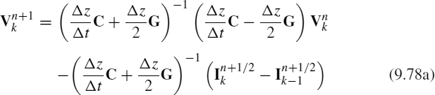
for k = 2, 3, ···, NDZ and

for k = 1, 2, ···, NDZ. The terminal voltages are, for resistive terminations, in the form of a generalized Thevenin equivalent given in (9.56),

and
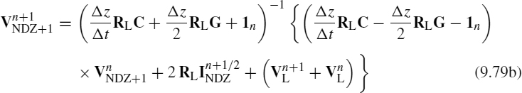
Equations (9.78a) and (9.79) are solved first to obtain the line voltages, and then the line currents are updated using (9.78b).
We next obtain the recursion relations for the FDTD formulation that includes frequency-dependent conductor losses. Since the second transmission-line equation in (9.73b) contains the dielectric losses in G, the voltage update equations for the interior voltages of a lossless MTL in (9.53b) are unchanged for the case of a lossless medium, G = 0n where 0n is the n × n zero matrix with zeros in every position:
![]()
for k = 2, 3, ···, NDZ. The terminal voltage update equations in (9.55) or in (9.57) for the generalized Thevenin equivalent characterization of the MTL terminations are also unchanged from the case of a lossless medium:
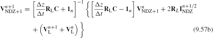
Only the equation for updating the current given in (9.53a) that is derived from the first MTL equation in (9.73a) that contains the conductor losses needs to be changed.
In the case of a multiconductor line containing imperfect conductors, a virtually identical development to the two-conductor line result in (8.180) provides the current update equations for lossy conductors:
for k = 1, ···, NDZ where
and the ai and bi are again determined with the Prony method and are given in Table 8.2 of Chapter 8. The matrix F is given by

This replaces equation (9.53a) of the lossless line development. The details of the derivation are essentially the same as for the lossy, two-conductor line given in Section 8.2.3 of Chapter 8. This is implemented in the FORTRAN code FDTDLOSS.FOR that is described in Appendix A.
9.2.4 Representation of the Lossy MTL with the Generalized Method of Characteristics
In Section 9.1.2, we discussed representing a lossless MTL with the generalized method of characteristics [2]. Decoupling the MTL equations with similarity trans-formations is easily accomplished for lossless MTLs. The generalized method of characteristics derived for lossless MTLs can be extended to lossy MTLs in the following manner but the details become more tedious. Again, we attempt to decouple the MTL equations for lossy lines by converting to modal quantities with similarity transformations:
where we have denoted the line voltages and currents as their Laplace-transformed variables. Substituting these into the MTL equations for a lossy line given in (9.69) yields


where the internal impedances of the conductors are included as the sum of the resistances and internal inductances as ![]() . If we can determine mode transformations such that the equations are uncoupled as
. If we can determine mode transformations such that the equations are uncoupled as
where ![]() and
and ![]() are diagonal, then the modal MTL equations in (9.82) are decoupled as
are diagonal, then the modal MTL equations in (9.82) are decoupled as

The mode voltages, ![]() , and mode currents, Îmi(z, s), are then represented with n separate, uncoupled, two-conductor, lossy lines. The diagonal per-unit-length impedance and admittance matrices for the modes in (9.83),
, and mode currents, Îmi(z, s), are then represented with n separate, uncoupled, two-conductor, lossy lines. The diagonal per-unit-length impedance and admittance matrices for the modes in (9.83), ![]() and
and ![]() , have entries
, have entries ![]() and [
and [![]() ] for i = 1, …, n on the main diagonal and zeros elsewhere. Hence, the solutions for the modes are
] for i = 1, …, n on the main diagonal and zeros elsewhere. Hence, the solutions for the modes are

where the mode characteristic impedances and propagation constants are

and
The solutions in (9.85) can be written in the matrix form as
where ![]() is the n × n characteristic impedance matrix for the modes, which is diagonal with
is the n × n characteristic impedance matrix for the modes, which is diagonal with ![]() on the main diagonal and zeros elsewhere, and
on the main diagonal and zeros elsewhere, and ![]() is an n × n diagonal matrix containing
is an n × n diagonal matrix containing ![]() on the main diagonal and zeros elsewhere. The n × 1 vectors of undetermined constants,
on the main diagonal and zeros elsewhere. The n × 1 vectors of undetermined constants, ![]() , have entries
, have entries ![]() that are, in general, functions of s. Evaluating (9.88) at z = 0 and at z =
that are, in general, functions of s. Evaluating (9.88) at z = 0 and at z = ![]() gives
gives
and
Adding and subtracting (9.89) and (9.90) yields
where
We can therefore use all the techniques developed in Chapter 8 for two-conductor, lossy lines to model these uncoupled mode lines. The uncoupled mode line solutions in (9.91) and (9.92) can be represented as shown in Figure 9.7. Time-domain representations of the frequency-dependent individual mode characteristic impedances ![]() as well as the propagation functions
as well as the propagation functions ![]() can be obtained with the Pade method or the Prony method as described in Chapter 8. This allows the use of the recursive convolution method to evaluate the convolutions that are represented by products of functions of s. In some cases, these can be represented with lumped RLCG circuits [15]. Controlled sources can, as for lossless lines in the earlier part of this chapter, be used to transform the mode voltages and currents from these uncoupled lines back to the actual line voltages and currents using (9.81) as illustrated in Figure 9.1. Hence, we can represent the lossy line and the transformations as shown in Figure 9.7.
can be obtained with the Pade method or the Prony method as described in Chapter 8. This allows the use of the recursive convolution method to evaluate the convolutions that are represented by products of functions of s. In some cases, these can be represented with lumped RLCG circuits [15]. Controlled sources can, as for lossless lines in the earlier part of this chapter, be used to transform the mode voltages and currents from these uncoupled lines back to the actual line voltages and currents using (9.81) as illustrated in Figure 9.1. Hence, we can represent the lossy line and the transformations as shown in Figure 9.7.

FIGURE 9.7 Illustration of the generalized method of characteristics for MTLs via decoupling.
This is very similar to the representation for the two-conductor lossless line shown in Figure 8.9 that was derived from the method of characteristics in Chapter 8 and produced the exact SPICE model of a two-conductor, lossless line. It is also used for a lossless MTL in Section 9.1.2 of this chapter. This representation is referred to in the literature as the generalized method of characteristics [15–27]. It should be noted that the vast majority of these works assume that the loss parameter matrices, R, Li, and G, are constant matrices, that is, independent of s and are therefore dc or low-frequency parameters. This is done to simplify the mathematics. But clearly, this is unrealistic since high-frequency skin-effect losses are neglected, as are the frequency-dependent losses in the surrounding dielectric medium. Incorporating the frequency-dependent losses of the conductors and dielectric medium obviously complicates the analysis rather severely but is a necessary, practical requirement. Investigation of the required relationship between ![]() and
and ![]() to ensure causality of the response is given in [28]. The method of numerical inversion of the Laplace transform is an alternative method of generating the time-domain functions and is discussed in [29–32]. Observe that a major difficulty with diagonalizing the MTL equations for a lossy line as in (9.83) is that, in general, the mode transformations will be frequency dependent and will be functions of s! Hence, the controlled sources in Figure 9.7 that implement the transformations back to actual line voltages and currents will represent convolutions. This presents a rather undesirable situation because we are faced with numerous convolutions when we convert the mode quantities back to actual line voltages and currents as in (9.81). Furthermore, it is difficult to compute the eigenvectors of a matrix (the columns of
to ensure causality of the response is given in [28]. The method of numerical inversion of the Laplace transform is an alternative method of generating the time-domain functions and is discussed in [29–32]. Observe that a major difficulty with diagonalizing the MTL equations for a lossy line as in (9.83) is that, in general, the mode transformations will be frequency dependent and will be functions of s! Hence, the controlled sources in Figure 9.7 that implement the transformations back to actual line voltages and currents will represent convolutions. This presents a rather undesirable situation because we are faced with numerous convolutions when we convert the mode quantities back to actual line voltages and currents as in (9.81). Furthermore, it is difficult to compute the eigenvectors of a matrix (the columns of ![]() and
and ![]() ) when the matrix is a function of s. To henceforth simplify the notation, we will denote the mode transformations as
) when the matrix is a function of s. To henceforth simplify the notation, we will denote the mode transformations as ![]() and
and ![]() with the understanding that these will, in general, be frequency dependent for lossy MTLs.
with the understanding that these will, in general, be frequency dependent for lossy MTLs.
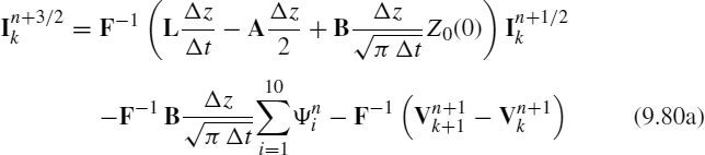
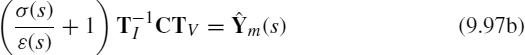
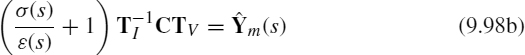
To avoid these convolutions in the mode transformations, we try to obtain frequency-independent modal transformations. There are some special cases where we can obtain frequency-independent mode transformations thereby simplifying the equivalent circuit in Figure 9.7. The mode transformations will then be frequency independent and hence the parameters of the controlled sources representing them in Figure 9.7 will be constants. First we write out (9.83), substituting ![]() :
:
Hence, we must determine two n × n constant transformation matrices TV and TI that simultaneously diagonalize five matrices, R, Li, L, G, and C. Clearly, this is too much to expect. Now let us make some assumptions to allow the decoupling of the MTL equations and, in addition, give frequency-independent transformations. The first assumption is that the surrounding medium is homogeneous, for example, a stripline. For a homogeneous medium, we have the identities

Next, we assume that the n conductors are identical leading to
where r0(s) and li0(s) represent the resistance and internal inductance, respectively, of the reference conductor and 1n is the n × n identity matrix and Un is the n × n unit matrix with ones in all positions. (Note: For a reference conductor not of finite size such as a ground plane, spreading of the return current will cause the off-diagonal terms to be unequal so that the forms in (9.95) will not apply.) The equations to be diagonalized in (9.93) reduce to

Hence, we must simultaneously diagonalize two matrices Un and C. In addition, the transformations must be such that ![]() is also diagonal. We can simultaneously diagonalize Un and C because both are real, symmetric, and positive definite (see Section 9.1.2.2). However, the product of the transformation matrices
is also diagonal. We can simultaneously diagonalize Un and C because both are real, symmetric, and positive definite (see Section 9.1.2.2). However, the product of the transformation matrices ![]() is not diagonal. Hence, we must make the following assumptions:
is not diagonal. Hence, we must make the following assumptions:
- n identical conductors ignoring loss in the reference conductor, that is, r0(s) = 0 and li0(s) = 0 or
- n + 1 identical conductors, that is, r0(s) = r(s) and li0(s) = li(s).
In the first case, the equations in (9.96) become
The transformations can be found that diagonalize all matrices in (9.97) as the following shows. Since C is a real, symmetric matrix, it can be diagonalized by an orthogonal transformation, as TtCT = Λ where Λ is an n × n diagonal matrix and T−1 = Tt where the superscript t denotes the transpose of the matrix (see Section 9.1.2.1). Hence, we can choose TV = T and ![]() so that
so that ![]() is diagonal. The matrix
is diagonal. The matrix ![]() , is automatically diagonalized:
, is automatically diagonalized: ![]()
![]() . Observe that
. Observe that ![]() is also automatically diagonalized.
is also automatically diagonalized.
In the second case the equations in (9.96) become
As C and (1n + Un) are symmetric matrices and C is positive definite, the transformations can be found that simultaneously diagonalize these two matrices as ![]() and
and ![]() where Λ1 and Λ2 are diagonal matrices resulting in uncoupled mode equations (see Section 9.1.2.2). The matrix,
where Λ1 and Λ2 are diagonal matrices resulting in uncoupled mode equations (see Section 9.1.2.2). The matrix, ![]() , is again automatically diagonalized:
, is again automatically diagonalized: ![]() .
.
Suppose, we assume that the n conductors are identical and that only the nearest neighbor coupling exists, that is, only adjacent lines are coupled. In addition, if the self-inductances are equal and the self-capacitances are equal, and if the mutual capacitances are equal and the mutual inductances are equal, then the C and L matrices are in the very special form as tridiagonal Toeplitz matrices, and we can choose the mode transformations to be identical as TV = TI = M and M−1 = Mt where t denotes the transpose [33, 34]. If all of the above special conditions are satisfied, then the C and L matrices are of the very special form:

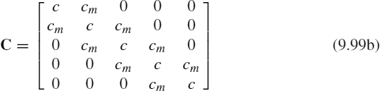
The coupled microstrip line is an example of this type of structure (although there exists coupling to some degree between all pairs of conductors). Furthermore, the entries in M are independent of the entries in C and L for this type of structure and are given in [33, 34]. This is a very special case of symmetry and is very similar to the case of cyclic-symmetric structures discussed in Section 7.2.2.5 of Chapter 7. Hence, the C and L matrices may be simultaneously diagonalized as MtLM = ΛL and MtCM = ΛC where ΛL and ΛC are diagonal matrices. Although this seems to decouple the general case of lines in an inhomogeneous medium, decoupling of the MTL equations requires that the conductor impedance matrices be of the form R + sLi = (r + sli) 1n, which means that we must also assume that all conductors are identical and neglect the loss in the reference conductor. In this case
Since C is a tridiagonal Toeplitz form, assuming only the nearest neighbor coupling seems to imply that we may also assume that G is a tridiagonal Toeplitz form. If that assumption is made, then the same M will also diagonalize G as

So if we assume (1) only nearest neighbor coupling, (2) all conductors are identical and neglect the loss in the reference conductor, and (3) special cross-sectional symmetry that yields the special forms of L and C in (9.99), then the MTL equations can be decoupled for an inhomogeneous medium with frequency-independent transformations. Furthermore, the transformations are general and are independent of the entries in L and C.
The case of cyclic-symmetric structures discussed in Section 7.2.2.5 of Chapter 7 is decoupleable by frequency-independent transformations. Frequency-independent transformations are given for these structures in Section 7.2.2.5. Cyclic-symmetric structures require that the n conductors be identical, for example, identical wire radii and insulation types and thicknesses as shown in Figure 7.1. The reference conductor can be different. Common cases are the case of two identical wires at the same height above a ground plane as shown in Figure 7.2(a) or the symmetrical microstrip line shown in Figure 7.2(b). For both of these structures, the impedance and admittance matrices have the form
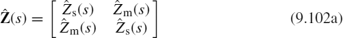
The frequency-independent transformation that diagonalizes these is

When none of the above special cases exist, the MTL equations including frequency-dependent losses cannot, in general, be decoupled with frequency-independent transformations. However, the method of characteristics developed earlier for lossless lines can be extended, using convolution, to the lossy line case to develop a 2n-port model of the lossy line. Consider the frequency-domain solution of the MTL equations given in (7.30) of Chapter 7 written in Laplace-transformed form substituting jω = s:
The characteristic admittance matrix ![]() is the inverse of the characteristic impedance matrix and is given in (7.32) as
is the inverse of the characteristic impedance matrix and is given in (7.32) as ![]() . The n × n matrix
. The n × n matrix ![]() diagonalizes the product of the frequency-domain per-unit-length impedance and admittance matrices as
diagonalizes the product of the frequency-domain per-unit-length impedance and admittance matrices as ![]() where the per-unit-length impedance and admittance matrices of the line are
where the per-unit-length impedance and admittance matrices of the line are ![]() and
and ![]() . All matrices and vectors are, in general, frequency dependent, that is, functions of s. Multiplying (9.104b) by the characteristic impedance matrix,
. All matrices and vectors are, in general, frequency dependent, that is, functions of s. Multiplying (9.104b) by the characteristic impedance matrix, ![]() , evaluating at z = 0 and z =
, evaluating at z = 0 and z = ![]() , and adding and subtracting the resulting equations gives
, and adding and subtracting the resulting equations gives
This gives the 2n-port equivalent circuit shown in Figure 9.8. Now, we convert to the time domain. Taking the inverse Laplace transform gives
where ![]() and
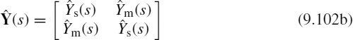
and ![]() and * denotes convolution. This gives another form of the generalized method of characteristics (without the necessity for the mode transformations) as the convolutions of the time-domain characteristic impedance matrix zC(t) and the time-domain delay matrix h(t) with port currents and voltages. The structure of this equivalent circuit in Figure 9.8 is virtually identical to that shown in Figure 8.9 for two-conductor lossless lines but with coupling between all lines. An alternative representation is obtained by premultiplying (9.105) by the characteristic admittance matrix
and * denotes convolution. This gives another form of the generalized method of characteristics (without the necessity for the mode transformations) as the convolutions of the time-domain characteristic impedance matrix zC(t) and the time-domain delay matrix h(t) with port currents and voltages. The structure of this equivalent circuit in Figure 9.8 is virtually identical to that shown in Figure 8.9 for two-conductor lossless lines but with coupling between all lines. An alternative representation is obtained by premultiplying (9.105) by the characteristic admittance matrix ![]() and rearranging to yield
and rearranging to yield


This gives the 2n-port equivalent circuit shown in Figure 9.9. Now, we convert to the time domain. Taking the inverse Laplace transform gives

FIGURE 9.8 An alternative form of the generalized method of characteristics.
where ![]() and
and ![]() and * denotes convolution. This gives another form of the generalized method of characteristics (without the necessity of mode transformations) as the convolutions of the time-domain characteristic admittance matrix yC(t) and the time-domain delay matrix f(t) with port currents and voltages.
and * denotes convolution. This gives another form of the generalized method of characteristics (without the necessity of mode transformations) as the convolutions of the time-domain characteristic admittance matrix yC(t) and the time-domain delay matrix f(t) with port currents and voltages.
Alternative representations of these in terms of the transformation matrix ![]() that diagonalizes the product
that diagonalizes the product ![]() as
as ![]() are obtained from the representation in (7.25) of Chapter 7:
are obtained from the representation in (7.25) of Chapter 7:
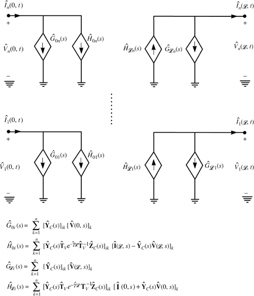
FIGURE 9.9 An alternative form of the generalized method of characteristics.
Eliminating the vectors of undetermined constants,![]() , as above gives
, as above gives

and, after multiplying by ![]() , alternatively
, alternatively
Using the methods in [B.25], it can be shown that
This demonstrates (as expected) that (9.105) and (9.110) are equivalent as are (9.107) and (9.111), even though one set of equations involves ![]() and the other set of equations involves
and the other set of equations involves ![]() . The article in [B.25] demonstrates the hazards in using quantities that involve both
. The article in [B.25] demonstrates the hazards in using quantities that involve both ![]() and
and ![]() rather than involving only
rather than involving only ![]() or
or ![]() . This has caused considerable confusion throughout the literature and the reader should be alert to these seemingly equivalent definitions. Many of the publications in the references use notation such as Si and Sv when not only are these different from the above
. This has caused considerable confusion throughout the literature and the reader should be alert to these seemingly equivalent definitions. Many of the publications in the references use notation such as Si and Sv when not only are these different from the above ![]() and
and ![]() but, even though it may be the case that
but, even though it may be the case that ![]() , it also turns out that
, it also turns out that ![]() and Si has an entirely different meaning.
and Si has an entirely different meaning.
9.2.5 Model Order Reduction (MOR) Methods
High-density interconnects in today's integrated circuits and digital systems contain an enormous number of coupled MTLs. The computational burden in using the above methods is becoming intractable. Hence, there is a need to reduce the order of the representation of these structures. These representations generally fit into the category of macromodels. Transfer functions of MTLs involve transcendental functions that have an infinite number of roots. Hence, these transfer functions will have an infinite number of poles making the inverse transforms impossible to compute. However, if we can represent these transfer functions with only a smaller, finite number of dominant poles, then the computational burden is reduced. This is generally referred to as Model Order Reduction or MOR. In this final section of the chapter, we will discuss some of the many MOR methods such as Pade approximations, asymptotic waveform evaluation or AWE, complex frequency hopping or CFH, and vector fitting or VF along with the synthesis of lumped equivalent circuits. The literature is rapidly expanding in terms of MOR techniques.
9.2.5.1 Pade Approximation of the Matrix Exponential
The MTL equations in Laplace transform form for a lossy line are coupled, ordinary differential equations given in (9.69) as


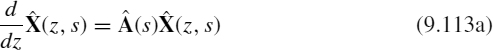
where ![]() is the internal impedance matrix for the conductor losses. These can be put into the so-called state-variable form as [13, 14]
is the internal impedance matrix for the conductor losses. These can be put into the so-called state-variable form as [13, 14]
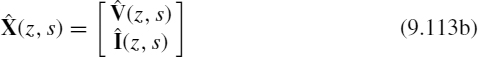
where ![]() is a 2n × 1 vector containing the voltages and currents of the line as
is a 2n × 1 vector containing the voltages and currents of the line as
![]() is a 2n × 2n matrix containing the line per-unit-length parameters as
is a 2n × 2n matrix containing the line per-unit-length parameters as
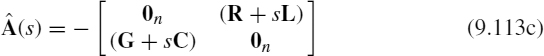
and 0n is the n × n zero matrix with zeros in all positions. In the following, we will, for the purposes of economy of notation, not continue to place the caret over the transformed per-unit-length parameters nor indicate that they are functions of s. Nor will we explicitly show the separation of the internal impedance into the resistance and internal inductance. All of this is implied.
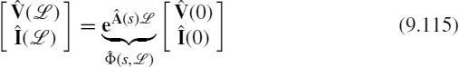
The solution to (9.113) is well known to be [A.2,13, 14]
where ![]() is the total line length. The 2n × 2n matrix
is the total line length. The 2n × 2n matrix ![]() is referred to in the circuits and automatic controls literature as the state-transition matrix. In our vernacular, this is equivalent to the chain-parameter matrix:
is referred to in the circuits and automatic controls literature as the state-transition matrix. In our vernacular, this is equivalent to the chain-parameter matrix:
The state-transition or chain-parameter matrix has the following infinite series expansion [A.2,13, 14]
and we denote the total line parameter matrix as
In Section 8.2.6 of the previous chapter, we discussed using the Pade method how to approximate a function F(s) as a rational function consisting of the ratio of Nth order polynomials in s as

where F(0) is the dc response at s = 0. We can determine the 2N parameters in this representation, a1, ···, aN, b1, ···, bN, by matching it to a Maclaurin expansion about s = 0 as an infinite series in s:
and the mi are said to be the “moments” of f(t). Equating (9.117) and (9.118) and multiplying both sides by the denominator gives

Matching powers of s gives the matrix equations given in equations (8.215) of Chapter 8:


The bi denominator coefficients for i = 1, ···, N can be obtained from (8.215a), and the ai numerator coefficients for i = 1, ···, N can then be obtained from (8.215b). (See Section 8.2.6 of Chapter 8 for this development.) We can use this result to obtain a Pade representation of the chain-parameter matrix. Each entry in the 2n × 2n chain-parameter matrix is represented as a rational function of s as a ratio of polynomials in s:
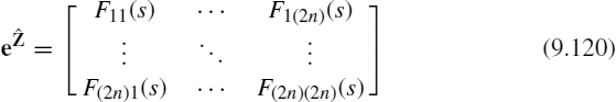
Rather than expanding the individual entries, we can obtain this in matrix form as
or
Comparing (9.116a) to 9.118) indicates that the “moments” of the expansion will be in the form of factorials, that is, mi = 1/i!. A closed-form solution for the Pade expansion polynomials can be obtained as powers of ![]() [35–37]
[35–37]

The general result for the orders of the numerator and denominator polynomials not being the same is given in [35–37]. In addition, it is shown in [36] that these representations and the associated model are passive. Passivity is a very important criterion for any simulation model and means that the system cannot generate more energy than it absorbs and that no passive termination on the system will make the system unstable. Recall from Chapter 8 that the Pade method may generate polynomials with unstable poles, that is, the denominator roots have positive real parts. For the above development, we are assured that no such instability will be generated. Furthermore, (9.122) gives a closed-form result for the expansions.
9.2.5.2 Asymptotic Waveform Evaluation (AWE)
The AWE method is also a moment-matching technique [35–39]. The method seeks to expand the Laplace-transformed voltages and currents in power series in the Laplace transform variable s, that is, in terms of moments. By matching matrix coefficients of corresponding powers of s, the MTL equations are transformed into a series of differential equations that can be solved iteratively or interfaced with a conventional circuit simulator such as SPICE.
For example, the chain-parameter matrix can be solved this way by writing out (9.116a) as
Expanding this and grouping terms that are associated with powers of s and comparing to a moment expansion as
gives recursion relations for the “moment matrices” ![]() [35].
[35].
Similarly, the transformed MTL equations in state-variable form given in (9.113) can be diagonalized as [41]

where ![]() is the diagonal matrix of propagation constants and
is the diagonal matrix of propagation constants and
or, in other words,
From this we identify the modal transformation matrices of Chapter 7 as
and
and ![]() is the characteristic impedance matrix. Hence, the solution of the first-order state-variable matrices in (9.114) becomes
is the characteristic impedance matrix. Hence, the solution of the first-order state-variable matrices in (9.114) becomes

and the chain-parameter matrix has been generated. This gives the form of the solution that is identical to (9.107):


and ![]() is the characteristic admittance matrix. Hence, the solution is representable again in the form of the generalized method of characteristics as shown in Figure 9.9.
is the characteristic admittance matrix. Hence, the solution is representable again in the form of the generalized method of characteristics as shown in Figure 9.9.
As an alternative to the use of Pade approximations to obtain the time-domain representations of ![]() and
and ![]() , we represent the various matrices in terms of moments about s = 0 as
, we represent the various matrices in terms of moments about s = 0 as
Substituting these moment expansions into (9.125) gives a recursion relation for the moments as [41]

The moments of the characteristic admittance matrix can be obtained by substituting the moment expansion given in (9.131) into (9.128)
to yield the recursion relation [41]
The moments of the propagation function ![]() can be similarly obtained. The time-domain results can be put in a form allowing a recursive convolution scheme to be implemented and can be stenciled into the modified nodal admittance (MNA) matrix of SPICE [43].
can be similarly obtained. The time-domain results can be put in a form allowing a recursive convolution scheme to be implemented and can be stenciled into the modified nodal admittance (MNA) matrix of SPICE [43].
9.2.5.3 Complex Frequency Hopping (CFH)
The transfer functions of transmission lines involve transcendental functions and therefore have an infinite number of poles. However, not all of these poles need to be used in a macromodel of the line as shown in the pole plot in Figure 9.10. The horizontal axis is the real part of s = σ + jω and the vertical axis is the imaginary part. For example, two real poles s1 = −1 and s2 = −1000 will have time-domain contributions in the response of e−t and e−1000t, respectively. The response due to the first pole s1 = −1 will take a much longer time to decay to zero than the response to the second pole s2 = −1000. Hence, poles that are further from the imaginary axis, s = jω, are less important in determining the time-domain response accurately. Conversely, the poles that are closer to the s = jω axis are more important in obtaining an accurate time-domain response and are called the dominant poles. It is important to determine only the dominant poles in order to obtain an accurate time-domain macromodel.
The Pade approximation is accurate only in a region of convergence about the expansion point. For example, if we expand the function in moments about s = 0 as in (9.118)
![]()
then the resulting Pade approximation in (9.117)

gives a good approximation only in a region of convergence about s = 0 as illustrated in Figure 10. The method of CFH seeks to determine the other dominant poles by redetermining the expansions by moving the regions of convergence along the s = jω axis as illustrated in Figure 10 [35, 44].
9.2.5.4 Vector Fitting
In obtaining a solution to differential equations (ordinary or partial), we discretize the time axis into Δ t intervals and recursively solve the equations. Performing a convolution generally requires the storage of all past time points, which is very burdensome in terms of memory requirements as well as computation time. In Section 8.2.3.4, we discussed the recursive convolution technique for evaluating convolution integrals, which avoids this problem. The recursive convolution method relies on representing the time-domain responses as the sum of exponential time functions such as
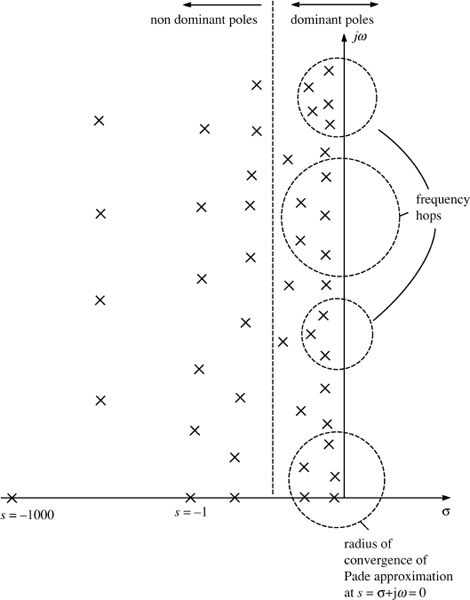
FIGURE 9.10 Illustration of the method of complex frequency hopping to determine the dominant poles.
The recursive convolution scheme relies on the property of the exponential e(a+b) = eaeb. For example, the convolution h(t)*x(t) is evaluated as
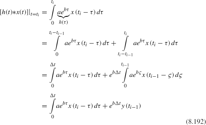
and we have used a change of variables, ![]() , in the second integral. Hence, the recursive convolution technique allows us to accumulate the values of the convolution at the previous time points as we proceed.
, in the second integral. Hence, the recursive convolution technique allows us to accumulate the values of the convolution at the previous time points as we proceed.
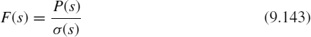
If we characterize a transfer function in the frequency domain in rational polynomial form as

it can be expanded using partial fractions as
where the pi are the poles and the ci are the residues. This becomes, in the time domain,

and hence, the recursive convolution scheme can be easily implemented. In order to determine the frequency-domain expansion in (9.136), we need to determine the dominant poles over the frequency range of interest and their residues as in (9.136b). The vector fitting method seeks to do this [45–47].
The vector fitting method uses an auxiliary undetermined rational function expanded as

and an approximation to F(s):

In both these functions, we choose a set of starting poles ![]() and write
and write
Writing this out yields
or

Choosing M frequency points, sk = jωk, over the frequency range of interest to evaluate this gives M equations in the 2N + 1 unknowns c0, ci, ![]() in the form
in the form
where
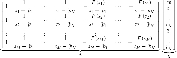
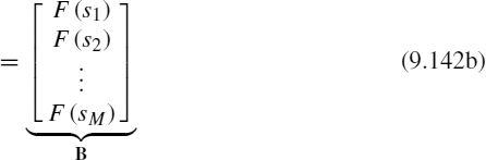
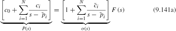
matrix A is M × (2N + 1), vector X is of length 2N + 1, and vector B is of length M. Rewriting (9.140) as
shows the key fact about the vector fitting method: the poles, pi of F(s) are the zeros of σ(s)! Also observe that the initial estimates of the poles ![]() cancel out! Hence, once (9.142) is solved for the N residues of σ(s),
cancel out! Hence, once (9.142) is solved for the N residues of σ(s), ![]() , the N zeros of σ(s) can be determined by multiplying out (9.138) and then factoring the numerator polynomial. An alternative, more direct, method is to determine the N poles of F(s), pi, as the N eigenvalues of the N × N matrix [47, 48]
, the N zeros of σ(s) can be determined by multiplying out (9.138) and then factoring the numerator polynomial. An alternative, more direct, method is to determine the N poles of F(s), pi, as the N eigenvalues of the N × N matrix [47, 48]
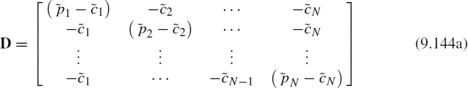
as
where || denotes the determinant of the enclosed matrix. These new poles are again used as the starting poles, and the process is repeated until the poles converge. The initial poles are typically chosen to be equally spaced, logarithmically, over the frequency range that we wish to characterize, and the real parts are chosen to be a factor of 100 smaller than the imaginary parts, that is, ![]() with βi = 100αi, as recommended in [45].
with βi = 100αi, as recommended in [45].
If we choose the number of frequency points for the sk, M, to be larger than the number of unknowns in X, 2N+1, (9.142) becomes an overdetermined set of equations, and the residues can be determined to minimize the error in a least-squares sense [49]. In a linear least-squares problem, we approximate a function as a linear combination of K basis functions ![]() i(s) as
i(s) as

Matching this to the known values of the function at M points, sj, where M ≥ K gives
This gives M equations in the K expansion coefficients, ai, written in matrix form as
where
where A is M × K, X is K × 1, and B is M × 1. Then, we determine the ai to minimize the square of the difference between ![]() and the values of the function at the M points, sj, as
and the values of the function at the M points, sj, as

To minimize this error, we differentiate (9.148) with respect to the ai and set the result equal to zero giving K equations as
This can be written as
where

This can be written in matrix form as
where t denotes transpose and the entries in A, X, and B are given in (9.147). The resulting equations in (9.151) are K equations in the K unknown expansion coefficients, ai. To avoid roundoff error, the preferred method of solution for (9.151) is singular value decomposition (SVD) [49].
The equations in (9.142) are in the form of (9.147) where the K ![]() (2N + 1)
(2N + 1) ![]() i(sj) are
i(sj) are

and the K ![]() (2N + 1) ai are
(2N + 1) ai are
and A is M × (2N + 1), X is (2N + 1) × 1, and B is M × 1. The resulting equations in the least-square method in (9.151) are 2N + 1 equations in the 2N + 1 residues in (9.152b). The starting poles are chosen and (9.151) is solved for the residues of σ(s) in (9.138), ![]() . The new poles are obtained as the eigenvalues of (9.144). These are used for the new starting poles, and the process is repeated. After convergence, F(s) is factored as in (9.136b), and the time-domain representation in terms of exponential functions is obtained as in (9.137). Any convolutions involving this function can then be evaluated using the method of recursive convolution.
. The new poles are obtained as the eigenvalues of (9.144). These are used for the new starting poles, and the process is repeated. After convergence, F(s) is factored as in (9.136b), and the time-domain representation in terms of exponential functions is obtained as in (9.137). Any convolutions involving this function can then be evaluated using the method of recursive convolution.
An alternative to using the recursive convolution scheme is to synthesize lumped equivalent circuits to represent F(s) thereby directly using programs such as SPICE to obtain the time-domain response of the system. Such representations of the frequency-domain factored form in (9.136b) are given in [50] using R, L, C elements and controlled sources.
9.3 COMPUTED AND EXPERIMENTAL RESULTS
The computed results are obtained for the time-domain responses of a three-wire ribbon cable (shown in cross section in Fig.7.10) and a three-land PCB (shown in cross section in Fig.7.13). The terminal configurations for both structures are shown in Figure 9.11. The conductors are numbered as shown in accordance with the numbering used to obtain the per-unit-length parameter matrices. A 50-Ω time-domain source produces an open-circuit voltage VS(t) that is in the form of a periodic trapezoidal waveform having a 50% duty cycle and equal rise and fall times with various values. The level of VS(t) will be 1 V in all cases. The source and load structure will be characterized with generalized Thevenin equivalents as
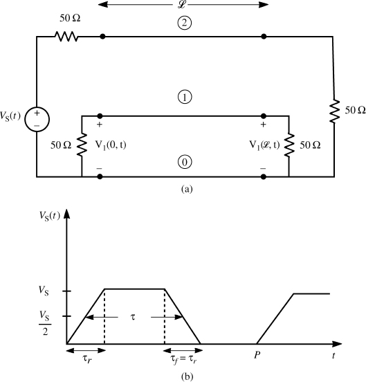
FIGURE 9.11 A three-conductor line for illustrating the predictions of various models: (a) terminal representations and (b) representation of the open-circuit voltage waveform of the source.

where

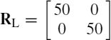
We will show the predictions of the lossless SPICE model, the lumped-Pi approximate model, the TDFD transformation method, and the FDTD method. These will be compared with oscilloscope photographs of the experimentally obtained results.
9.3.1 Ribbon Cables
The cross section of the three-wire ribbon cable is shown in Figure 7.10 and the per-unit-length parameters are computed using RIBBON.FOR that is described in Appendix A and given in Chapter 5 as
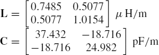
The pulse rise/fall times are 20 ns and the line length is ![]() = 2m. The mode velocities of propagation computed with SPICEMTL.FOR are vm1 = 2.324 × 10⁸ m/s and vm2 = 2.5106 × 10⁸ m/s giving one-way time delays of the modes of TDm1 = 8.606 ns and TDm2 = 7.996 ns. The characteristic impedances of the modes are ZCm1 = 91.96 Ω and ZCm2 = 254.93 Ω.
= 2m. The mode velocities of propagation computed with SPICEMTL.FOR are vm1 = 2.324 × 10⁸ m/s and vm2 = 2.5106 × 10⁸ m/s giving one-way time delays of the modes of TDm1 = 8.606 ns and TDm2 = 7.996 ns. The characteristic impedances of the modes are ZCm1 = 91.96 Ω and ZCm2 = 254.93 Ω.

FIGURE 9.12 Oscilloscope photograph of the experimentally determined near-end crosstalk for the ribbon cable of Figure 7.10 and a pulse rise time of 20 ns.
Figure 9.12 shows an oscilloscope photograph of the near-end crosstalk voltage V1(0, t). The crosstalk waveform rises to a peak of around 110 mV. Figure 9.13(a) shows a comparison of the predictions of (a) SPICE using SPICEMTL.FOR to generate the PSPICE subcircuit model as described in Section 9.1.2, (b) one Pi section lumped model generated by SPICELPI.FOR to generate the PSPICE subcircuit model as described in Section 9.1.3, and (c) the Branin recursive solution model given in Section 9.1.1. All three models assume a lossless line and the Branin model also assumes a homogeneous medium. The SPICE model predicts the experimentally obtained waveform in Figure 9.12 very well. The peak voltage is also predicted to be 110 mV. The one-section lumped-Pi model predicts the general shape of the waveform, but there is some error around the peak. This is to be expected since the spectral content of the input pulse is on the order of BW = 1/τr = 50 MHz. The line length of 2 m is on the order of (1/2.3)λ at 50 MHz using the smaller of the mode velocities of vm1 = 2.324 × 10⁸ m/s. Branin's recursive solution method also predicts the general waveform shape but does not agree with the SPICE solution as it should. This is because, as discussed in Section 9.1.1, Branin's recursive solution as implemented in BRANIN.FOR requires that we assume a homogenous medium (logically free space). Figure 9.13(b) shows the comparison where we ignore the dielectric insulations and recompute the per-unit-length parameters and the resulting SPICE solution for free space surrounding the wires. The results are now identical as they should be.
Figure 9.14 shows the predictions of the TDFD prediction model described in Section 9.1.4. This model is implemented using TIMEFREQ.FOR. The values of the frequency-domain transfer function at the harmonics of the input pulse that are input to this program were computed, for a lossless line, using the SPICE code above to compute in the .AC mode. Various numbers of harmonics are used to recombine the sinusoidal components of the trapezoidal pulse train for a fundamental frequency of f0 = 1 MHz. (Actually, it does not matter what repetition frequency is used so long as the response to the rising edge, which is shown in the figure, has died out sufficiently before the response to the trailing edge occurs.) The predictions using 100 and 50 harmonics are virtually identical to the exact SPICE results. The predictions using 10 and 20 harmonics are poor. The spectrum of the trapezoidal pulse train begins rolling off at −40 dB/decade above a frequency of 1/π τr = 15.9 MHz giving a bandwidth on the order of 1/τr = 50 MHz. Hence, we require at least 50 harmonics of the fundamental repetition frequency of f0 = 1 MHz in order to capture the important spectral content.
Figure 9.15 shows the predictions of the FDTD model discussed in Section 9.1.5. This model is implemented using FINDIF.FOR for a lossless line. The line is discretized spatially into NDZ sections of length Δz = ![]() /NDZ. We chose NDZ = 2 so that each Δz = 1m section length was on the order of Δz < (1/5)λ at 50 MHz. The time discretization Δt must satisfy the Courant condition, that is,
/NDZ. We chose NDZ = 2 so that each Δz = 1m section length was on the order of Δz < (1/5)λ at 50 MHz. The time discretization Δt must satisfy the Courant condition, that is,
![]()
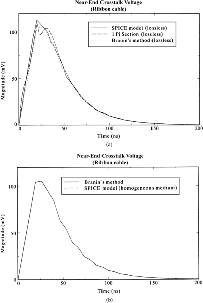
FIGURE 9.13 Comparison of the time-domain response of the near-end crosstalk of the lossless ribbon cable of Figure 7.10 determined (a) via the SPICE model, the lumped-Pi model, and Branin's series method implemented for a pulse rise time of 20 ns and (b) for a homogeneous medium.
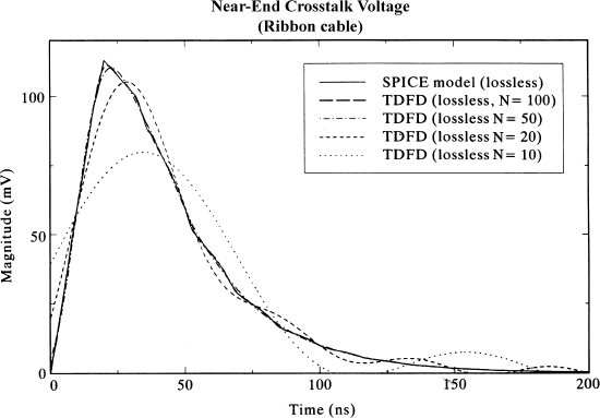
FIGURE 9.14 Comparison of the predictions of the SPICE model and the time-domain to frequency-domain transformation method for various numbers of harmonics for the lossless ribbon cable of Figure 7.10 for a pulse risetime of 20 ns.
For a final solution time of 200 ns, using the larger of the mode velocities, vm2 = 2.5106 × 10⁸ m/s, we obtain NDT ≥ 50. The predictions for NDZ = 2 and NDT = 50 give reasonable correlation with the exact SPICE predictions. The results for NDT = 500 are also shown and are virtually identical to the exact SPICE results.
These lumped-Pi, TDFD, and FDTD predictions were repeated to include the line losses. The predictions for the lumped-Pi model including the dc resistances of the conductors are compared to the SPICE (lossless) predictions in Figure 9.16 for one and two Pi sections used to represent the 2-m line length. Both the one-Pi model and the two-Pi model show some error around the peak of the waveform with the one-Pi model showing more error as expected. (Later predictions of the TDFD and FDTD models including losses will show that the SPICE predictions for a lossless line are very close to the actual results when losses are included.) The radius of one of the #36 gauge strands is 2.5 mils giving a dc resistance of each wire (dividing the resistance of each strand by the number in parallel, 7) as 0.3888 Ω. The frequency of onset of the ![]() increase is where the radius of a strand is equal to two skin depths or 4.3 MHz. Hence, using only the dc resistance in these lumped-Pi models will incur some poor predictions at the higher frequencies of the pulse spectrum.
increase is where the radius of a strand is equal to two skin depths or 4.3 MHz. Hence, using only the dc resistance in these lumped-Pi models will incur some poor predictions at the higher frequencies of the pulse spectrum.
Figure 9.17 shows the predictions of the TDFD and FDTD models as before but including the conductor losses. The lossy frequency-domain transfer function that is passed to the TDFD program, TIMEFREQ.FOR, was computed using MTL.FOR. The FDTD predictions including losses were obtained using FDTDLOSS.FOR. All models give approximately the same results, and the conductor losses appear to be inconsequential for this structure, line length, and pulse parameters. The losses give a dc offset during the time when the input pulse is in its 1-V steady state, which is referred to as common-impedance coupling. This level can be accurately predicted by modeling the line as simply its total dc resistances of 0.3888 Ω as shown in the next chapter to be around 2 mV.
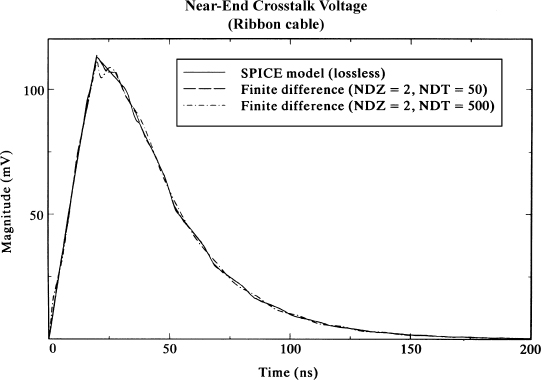
FIGURE 9.15 Comparison of the predictions of the SPICE model and the FDTD method for the lossless ribbon cable of Figure 7.10 for a pulse rise time of 20 ns.
Figure 9.18 shows the predictions of the TDFD and FDTD models including losses for pulse rise/fall times of 1 ns. The bandwidth of the pulse is 1/τr = 1 GHz. The TDFD program uses a repetition rate of f0 = 1 MHz, and hence 1000 harmonics are recombined in TIMEFREQ.FOR. The FDTD program breaks the 2-m line length into
![]()
sections giving 2m/Δz = 86. Hence, we chose NDZ = 100. The magic time step is NDT = 2511. The results are shown in Figure 9.18 giving very good accuracy for both prediction methods. Again, the effect of the conductor losses is to give an offset of around 2 mV when the pulse is in its steady state of 1 V.
9.3.2 Printed Circuit Boards
The cross section of the three-land PCB is shown in Figure 7.13 and the per-unit-length parameters are computed using PCB.FOR that is described in Appendix A as
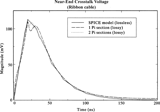
FIGURE 9.16 Comparison of the time-domain response of the near-end crosstalk of the ribbon cable of Figure 7.10 determined via the SPICE model (lossless) and the lumped-Pi model (dc losses included) using one and two sections to represent the line for a pulse rise time of 20 ns.
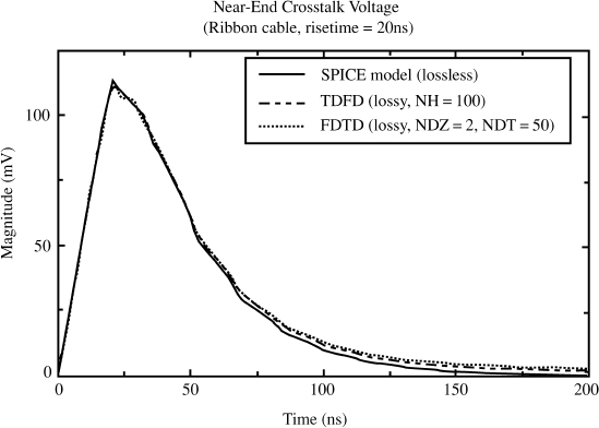
FIGURE 9.17 Comparison of the time-domain response of the near-end crosstalk of the ribbon cable of Figure 7.10 determined via the SPICE model (lossless), the time-domain to frequency-domain method (with skin effect losses), and the FDTD method (with skin effect losses) for a pulse rise time of 20 ns.
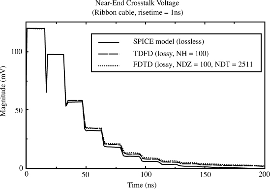
FIGURE 9.18 Comparison of the time-domain response of the near-end crosstalk of the ribbon cable of Figure 7.10 determined via the SPICE model (lossless), the time-domain to frequency-domain method (with skin effect losses), and the FDTD method (with skin effect losses) for a pulse rise time of 1 ns.

FIGURE 9.19 Oscilloscope photograph of the experimentally determined near-end crosstalk for the printed circuit board of Figure 7.13 and a pulse rise time of 6.25 ns.
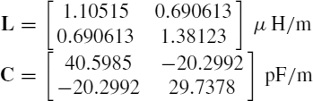
The pulse rise-/fall times are 6.25 ns and the line length is ![]() = 10 in. = 0.254 m. The mode velocities of propagation computed with SPICEMTL.FOR are vm1 = 1.8005 × 10⁸ m/s and vm2 = 1.9225 × 10⁸ m/s giving one-way time delays of the modes of TDm1 = 1.4108 ns and TDm2 = 1.3212 ns. The characteristic impedances of the modes are ZCm1 = 109.45 Ω and ZCm2 = 265.54 Ω.
= 10 in. = 0.254 m. The mode velocities of propagation computed with SPICEMTL.FOR are vm1 = 1.8005 × 10⁸ m/s and vm2 = 1.9225 × 10⁸ m/s giving one-way time delays of the modes of TDm1 = 1.4108 ns and TDm2 = 1.3212 ns. The characteristic impedances of the modes are ZCm1 = 109.45 Ω and ZCm2 = 265.54 Ω.
Figure 9.19 shows an oscilloscope photograph of the near-end crosstalk voltage, V1(0, t). The crosstalk waveform rises to a peak of around 95 mV. Figure 9.20 shows a comparison of the predictions of (a) SPICE using SPICEMTL.FOR to generate the PSPICE subcircuit model as described in Section 9.1.2, (b) one Pi section lumped model generated by SPICELPI.FOR to generate the PSPICE subcircuit model as described in Section 9.1.3, and (c) the Branin recursive solution model given in Section 9.1.1. All three models assume a lossless line and the Branin model also assumes a homogeneous medium. The SPICE model predicts the experimentally obtained waveform in Figure 9.19 very well. The peak voltage is also predicted to be 95 mV. The one-section lumped-Pi model predicts the general shape of the waveform but there is some error particularly around the peak. This is to be expected since the spectral content of the input pulse is on the order of BW = 1/τr = 160 MHz. The line length of .254 m is on the order of (1/5)λ at 160 MHz using the smaller of the mode velocities of vm1 = 1.8005 × 10⁸ m/s. Branin's recursive solution method also predicts the general waveform shape but does not agree with the SPICE solution because, as discussed previously, it neglects the inhomogeneous surrounding medium.
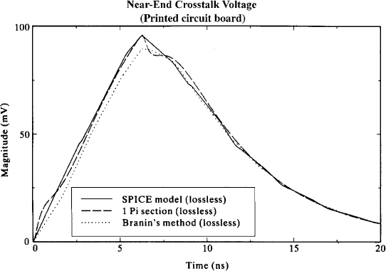
FIGURE 9.20 Comparison of the time-domain response of the near-end crosstalk of the lossless printed circuit board of Figure 7.13 determined via the SPICE model, the lumped-Pi model, and Branin's series method implemented for a pulse rise time of 6.25 ns and for a homogeneous medium.

FIGURE 9.21 Comparison of the predictions of the SPICE model and the time-domain to frequency-domain transformation method for various numbers of harmonics for the lossless printed circuit board of Figure 7.13 for a pulse rise time of 6.25 ns.
Figure 9.21 shows the predictions of the TDFD prediction model described in Section 9.1.4. This model is implemented using TIMEFREQ.FOR. The values of the frequency-domain transfer function at the harmonics of the input pulse that are input to this program were computed, for a lossless line, using the SPICE code above to compute in the .AC mode. Various numbers of harmonics are used to recombine the sinusoidal components of the trapezoidal pulse train for a fundamental frequency of f0 = 1 MHz. The predictions using 300 and 150 harmonics are virtually identical to the exact SPICE results. The predictions using 25 and 50 harmonics are poor. The spectrum of the trapezoidal pulse train begins rolling off at −40 dB/decade above a frequency of 1/πτr = 51 MHz giving a bandwidth on the order of 1/τr = 160 MHz. Hence, we require at least 160 harmonics of the fundamental repetition frequency of f0 = 1 MHz in order to capture the important spectral content.
Figure 9.22 shows the predictions of the FDTD model discussed in Section 9.1.5. This model is implemented using FINDIF.FOR for a lossless line. The line is discretized spatially into NDZ sections of length Δz = ![]() /NDZ. We chose NDZ = 2 so that each Δz = 0.127 m section length was on the order of Δz < (1/10)λ at 160 MHz.. The time discretization Δt must satisfy the Courant condition, that is,
/NDZ. We chose NDZ = 2 so that each Δz = 0.127 m section length was on the order of Δz < (1/10)λ at 160 MHz.. The time discretization Δt must satisfy the Courant condition, that is,

FIGURE 9.22 Comparison of the predictions of the SPICE model and the FDTD method for the lossless printed circuit board of Figure 7.13 for a pulse rise time of 6.25 ns.
![]()
For a final solution time of 40 ns, using the larger of the mode velocities, vm2 = 1.9225 × 10⁸ m/s, we obtain NDT ≥ 60. The predictions for NDZ = 2 and NDT = 60 give reasonable correlation with the exact SPICE predictions. The results for NDT = 600 are also shown and are virtually identical to the exact SPICE results.
These lumped-Pi, TDFD, and FDTD predictions were repeated to include the line losses. The predictions for the lumped-Pi model including the dc resistances of the conductors are compared to the SPICE (lossless) predictions in Figure 9.23 for one and two Pi sections used to represent the 0.254 m line length. Both the one-Pi model and the two-Pi model show some error around the peak of the waveform with the one-Pi model showing more error as expected. (Later predictions of the TDFD and FDTD models including losses will show that the SPICE predictions for a lossless line are very close to the actual results when losses are included.) The dc resistance of each land (width of 15 mils and thickness of 1.38 mils) is 0.328 Ω. The frequency of onset of the ![]() increase is approximated as where the thickness of each land is equal to two skin depths or 14.218 MHz. Hence, using only the dc resistance in these lumped-Pi models will incur some poor predictions at the higher frequencies of the pulse spectrum.
increase is approximated as where the thickness of each land is equal to two skin depths or 14.218 MHz. Hence, using only the dc resistance in these lumped-Pi models will incur some poor predictions at the higher frequencies of the pulse spectrum.

FIGURE 9.23 Comparison of the time-domain response of the near-end crosstalk of the printed circuit board of Figure 7.13 determined via the SPICE model (lossless) and the lumped-Pi model (dc losses included) using one and two sections to represent the line for a pulse rise time of 6.25 ns.
Figure 9.24 shows the predictions of the TDFD and FDTD models as before but including the conductor losses. The lossy frequency-domain transfer function that is passed to the TDFD program, TIMEFREQ.FOR, was computed using MTL.FOR. The FDTD predictions including losses were obtained using FDTDLOSS.FOR. All models give approximately the same results, and the conductor losses again appear to be inconsequential for this structure, line length, and pulse parameters. The losses again give a dc offset during the time when the input pulse is in its 1-V steady state, which is referred to as common-impedance coupling. This level can be accurately predicted by modeling the line as simply its total dc resistances of 0.328 Ω as shown in the next chapter to be around 2 mV.
Figure 9.25 shows the predictions of the TDFD and FDTD models including losses for pulse rise/fall times of 50 ps. The bandwidth of the pulse is 1/τr = 20 GHz. The TDFD program uses a repetition rate of f0 = 10 MHz, and hence 1000 harmonics are recombined in TIMEFREQ.FOR. The FDTD program breaks the 0.254-m line length into
![]()
sections giving 0.254 m/Δz = 282. Hence, we chose NDZ = 280. The magic time step is NDT = 6358. The results are shown in Figure 9.25 giving very good accuracy for both prediction methods. Again, the effect of the conductor losses is to give an offset of around 2 mV when the pulse is in its steady state of 1 V.
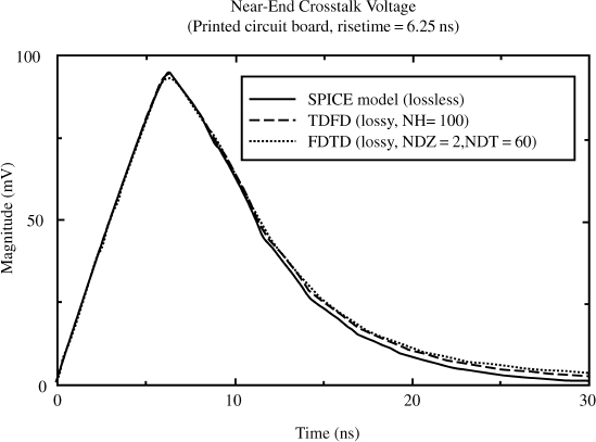
FIGURE 9.24 Comparison of the time-domain response of the near-end crosstalk of the printed circuit board of Figure 7.13 determined via the SPICE model (lossless), the time-domain to frequency-domain method (with skin effect losses), and the FDTD method (with skin effect losses) for a pulse rise time of 6.25 ns.
PROBLEMS
9.1 Derive the recursive relations given in (9.21a) and (9.21b).
9.2 Consider a lossless two-conductor line that has RS = 300Ω, RL = 60Ω, ZC = 100Ω, v = 300m/μs, ![]() = 300m, and vS(t) = 400u(t), where u(t) is the unit step function. Sketch V(0, t), I(0, t), V(
= 300m, and vS(t) = 400u(t), where u(t) is the unit step function. Sketch V(0, t), I(0, t), V(![]() , t), I(
, t), I(![]() , t) for 0 ≤ t ≤ 10μs. Do the results converge to the expected steady-state values? Confirm your results using PSPICE. [For voltage: ΓS = 1/2, ΓL = −1/4, Vinit = 100. For current: ΓS = −1/2, ΓL = 1/4, Iinit = 1. V(0, t)SS = V(
, t) for 0 ≤ t ≤ 10μs. Do the results converge to the expected steady-state values? Confirm your results using PSPICE. [For voltage: ΓS = 1/2, ΓL = −1/4, Vinit = 100. For current: ΓS = −1/2, ΓL = 1/4, Iinit = 1. V(0, t)SS = V(![]() , t)SS = 66.67, I(0, t)SS = I(
, t)SS = 66.67, I(0, t)SS = I(![]() , t)SS = 1.11]
, t)SS = 1.11]
9.3 Repeat Problem 9.2 for RL = 0 (short-circuit load). Confirm your results using PSPICE. [For voltage: ΓS = 1/2, ΓL = −1, Vinit = 100. For current: ΓS = −1/2, ΓL = 1, Iinit = 1. V(0, t)SS = V(![]() , t)SS = 0, I(0, t)SS = I(
, t)SS = 0, I(0, t)SS = I(![]() , t)SS = 1.333]
, t)SS = 1.333]
9.4 Repeat Problem 9.2 for RL = ∞ (open-circuit load). Confirm your results using PSPICE. [For voltage: ΓS = 1/2, ΓL = 1, Vinit = 100. For current: ΓS = −1/2, ΓL = −1, Iinit = 1. V(0, t)SS = V(![]() , t)SS = 400, I(0, t)SS = I(
, t)SS = 400, I(0, t)SS = I(![]() , t)SS = 0]
, t)SS = 0]

FIGURE 9.25 Comparison of the time-domain response of the near-end crosstalk of the printed circuit board of Figure 7.13 determined via the SPICE model (lossless), the time-domain to frequency-domain method (with skin effect losses), and the FDTD method (with skin effect losses) for a pulse rise time of 50 ps.
9.5 Confirm the diagonalization matrix for a real, symmetric matrix given in (9.37).
9.6 Determine the transformation T that diagonalizes L as TtLT = Lm where
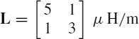
[T(1, 1) = T(2, 2) = 0.92388, T(1, 2) = −T(2, 1) = −0.382683, Lm(1, 1) = 5.414E − 6, Lm(2, 2) = 2.586E − 6]
9.7 Determine the transformation T that diagonalizes C as TtCT = Cm where

[T(1, 1) = T(2, 2) = 0.85065, T(1, 2) = −T(2, 1) = −0.525731, Cm(1, 1) = 6.90983E − 12, Cm (2, 2) = 18.0902E − 12]
9.8 Determine the TV and TI that simultaneously diagonalize the L and C in Problems 9.6 and 9.7 as ![]() and
and ![]() . [TV(1, 1) = 0.745356, TV(1, 2) = −0.942809, TV(2, 1) = 0.745356, TV(2, 2) = 0.4714, TI(1, 1) = 0.447214, TI(1, 2) = −0.707107, TI(2, 1) = 0.894427, TI(2, 2) = 0.707107, Lm(1, 1) = 4.2E − 6, Lm(2, 2) = 3.0E − 6, Cm(1, 1) = 8.333E − 12, Cm(2, 2) = 16.667E − 12]
. [TV(1, 1) = 0.745356, TV(1, 2) = −0.942809, TV(2, 1) = 0.745356, TV(2, 2) = 0.4714, TI(1, 1) = 0.447214, TI(1, 2) = −0.707107, TI(2, 1) = 0.894427, TI(2, 2) = 0.707107, Lm(1, 1) = 4.2E − 6, Lm(2, 2) = 3.0E − 6, Cm(1, 1) = 8.333E − 12, Cm(2, 2) = 16.667E − 12]
9.9 Determine the TV and TI that simultaneously diagonalize L and C as ![]() and
and ![]() where
where
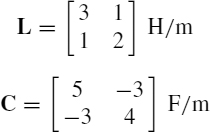
[TV(1, 1) = 1.10055, TV(1, 2) = 0.607046, TV(2, 1) = −0.1438, TV(2, 2) = 0.929182, TI(1, 1)=0.837174, TI(1, 2)=0.129561, TI(2, 1) = −0.546936, TI(2, 2) = 0.991571, Lm(1, 1) = 1.7851, Lm(2, 2) = 2.27372, Cm(1, 1) = 7.0883, Cm(2, 2) = 1.9117]
9.10 Consider the three-conductor line shown in Figure P9.10. The driven or generator conductor is a #20 gauge solid wire (radius 16 mils) and the pickup or receptor wire is a #28 gauge solid wire (radius 6.3 mils). The wires are separated by 1.5 cm and are suspended above an infinite, perfectly conducting ground plane at heights of 2 cm and 1 cm as shown. The lines are terminated as shown and are driven by a ramp voltage source. Neglect all losses, assume a homogeneous medium, and compute and plot versus time the near-end and far-end coupled voltages, VNE(t) and VFE(t), by the following methods: (a) a PSPICE model using SPICEMTL.FOR to generate a PSPICE subcircuit model, (b) Branin's method using BRANIN.FOR, (c) the TDFD transformation method using TIMEFREQ.FOR, and (d) the FDTD method using FINDIF.FOR.
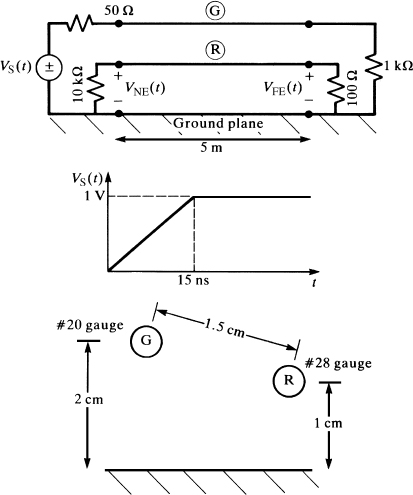
FIGURE P9.10
9.11 Recompute the SPICE results in Figure 9.6(a) and 9.6(b).
9.12 Verify the FDTD recursion relations in (9.78) and (9.79).
9.13 Verify the FDTD recursion relations in (9.53b), (9.57), and (9.80).
9.14 Verify the generalized method of characteristics results in (9.91) and (9.92).
9.15 Determine the transformation matrix that diagonalizes a 3 × 3 L as MtLM having the general Toeplitz form given in (9.99a).
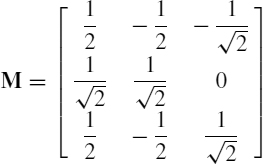
9.16 Show that the transformation matrices in (9.103) diagonalize the per-unit-length matrices in (9.102).
9.17 Derive the forms of the generalized method of characteristics given in (9.105), (9.107), (9.110), and (9.111).
9.18 Derive the result in (9.122).
9.19 Derive the Vector Fitting result in (9.142) and (9.144).
9.20 Derive the least-squares result in (9.151).
9.21 Using BRANIN.FOR, SPICEMTL.FOR, and SPICELPI.FOR, reproduce the results for the ribbon cable shown in Figure 9.13(a).
9.22 Using SPICEMTL.FOR and TIMEFREQ.FOR, reproduce the results for the ribbon cable shown in Figure 9.14.
9.23 Using SPICEMTL.FOR and FINDIF.FOR, reproduce the results for the ribbon cable shown in Figure 9.15.
9.24 Using SPICEMTL.FOR, TIMEFREQ.FOR (and MTL.FOR), and FDTDLOSS.FOR, reproduce the results for the ribbon cable shown in Figure 9.17.
9.25 Using BRANIN.FOR, SPICEMTL.FOR, and SPICELPI.FOR, reproduce the results for the PCB shown in Figure 9.20.
9.26 Using SPICEMTL.FOR and TIMEFREQ.FOR, reproduce the results for the PCB shown in Figure 9.21.
9.27 Using SPICEMTL.FOR and FINDIF.FOR, reproduce the results for the PCB shown in Figure 9.22.
9.28 Using SPICEMTL.FOR, TIMEFREQ.FOR (and MTL.FOR), and FDTDLOSS.FOR, reproduce the results for the PCB shown in Figure 9.24.
REFERENCES
[1] H. Amemiya, Time domain analysis of multiple parallel transmission lines, RCA Review, 28, 241–276, 1967.
[2] F.Y. Chang, Transient analysis of lossless coupled transsmision lines in inhomogeneous dielectric media, IEEE Transactions on Microwave Theory and Techniques, 18 (9), 616–626, 1970.
[3] C.W. Ho, Theory and computer-aided analysis of lossless transmission lines, IBM Journal of Research and Development, 17, 249–255, 1973.
[4] K.D. Marx, Propagation modes, equivalent circuits, and characteristic terminations for multiconductor transmission lines with inhomogeneous dielectrics, IEEE Transactions on Microwave Theory and Techniques, 21 (7), 450–457, 1973.
[5] H.W. Dommel and W. S. Meyer, Computation of electromagnetic transients, Proceedings of IEEE, 62 (7), 983–993, 1974.
[6] A.J. Gruodis, Transient analysis of uniform resistive transmission lines in a homogeneous medium, IBM Journal of Research and Development, 23 (6), 675–681, 1979.
[7] A.J. Gruodis and C. S. Chang, Coupled lossy transmission line characterization and simulation, IBM Journal of Research and Development, 25 (1) 25–41, 1981.
[8] A.R. Djordjevic, T.S., Sarkar, and R.F. Harrington, Analysis of lossy transmission lines with arbitrary nonlinear terminal networks, IEEE Transactions on Microwave Theory and Techniques, 34 (6), 660–666, 1986.
[9] A.R. Djordjevic, T.S. Sarkar, and R.F. Harrington, Time-domain response of multiconductor transmission lines, Proceedings of IEEE, 75 (6), 743–764, 1987.
[10] A. Ralston, A First Course in Numerical Analysis, McGraw-Hill, New York, 1965.
[11] V.K. Tripathi and J.B. Rettig, A SPICE model for multiple coupled microstrips and other transmission lines, IEEE Transactions on Microwave Theory and Techniques, 33 (12), 1513–1518, 1985.
[12] M.N.O. Sadiku, Numerical Techniques in Electromagnetics, CRC Press, Boca Raton, FL, 1992.
[13] L.O. Chua and P.M. Lin, Computer Aided Analysis of Electronic Circuits: Algorithms and Computational Techniques, Prentice-Hall, Englewood Cliffs, NJ, 1975.
[14] B.J. Leon, Lumped Systems, Holt, Rinehart, and Winston, New York, 1968.
[15] F.Y. Chang, Waveform relaxation analysis of RLCG transmission lines, IEEE Transactions on Circuits and Systems, 37 (11), 1394–1415, 1990.
[16] F.-Y. Chang, The generalized method of characteristics for waveform relaxation analysis of lossy coupled transmission lines, IEEE Transactions on Microwave Theory and Techniques, 37 (12), 2028–2038, 1989.
[17] V.K. Tripathi and A. Hill, Equivalent circuit modeling of losses and dispersion in single and coupled lines for microwave and millimeter-wave integrated circuits, IEEE Transactions on Circuits and Systems, 36 (2), 256–262, 1988.
[18] N. Orhanovic, V.K. Tripathi, and P. Wang, Generalized method of characteristics for time domain simulation of multiconductor lossy transmission lines, Proceedings of the IEEE Symposium on Circuits and Systems, 2388–2391, 1990.
[19] F.Y. Chang, Waveform relaxation analysis of nonuniform lossy transmission lines characterized with frequency-dependent parameters, IEEE Transactions on Circuits and Systems, 38 (12), 1484–1500, 1991.
[20] F.Y. Chang, Relaxation simulation of transverse electromagnetic wave propagation in coupled transmission lines, IEEE Transactions on Circuits and Systems, 38 (8), 916–936, 1991.
[21] C. Gordon, T. Blazek, and R. Mittra, Time-domain simulation of multiconductor transmission lines with frequency-dependent losses, IEEE Transactions on Computer-Aided Design, 11 (11), 1372–1387, 1992.
[22] F.Y. Chang, Transient simulation of nonuniform coupled lossy transmission lines characterized with frequency-dependent parameters part II: Discrete-time analysis, IEEE Transactions on Circuits and Systems, 39 (11), 907–927, 1992.
[23] S. Lin and E.S. Kuh, Transient simulation of lossy interconnects based on the recursive convolution formulation, IEEE Transactions on Circuits and Systems-I: Fundamental Theory and Applications, 39 (11), 879–892, 1992.
[24] V.K. Tripathi and N. Orhanovic, Time-domain characterization and analysis of dispersive dissipative interconnects, IEEE Transactions on Circuits and Systems, 39 (11), 938–945, 1992.
[25] J.I. Alonso, J.B. Borja, and F. Perez, A universal model for lossy and dispersive transmission lines for time domain CAD of circuits, IEEE Transactions on Microwave Theory and Techniques, 40 (5), 938–946, 1992.
[26] J. Mao and Z. Li, Analysis of the time response of multiconductor transmission lines with frequency-dependent losses by the method of convolution characteristics, IEEE Transactions on Microwave Theory and Techniques, 40 (4), 637–644, 1992.
[27] F.Y. Chang, Transient simulation of frequency-dependent nonuniform coupled lossy transmission lines, IEEE Transactions on Components, Packaging, and Manufacturing Technology. 17 (1), 3–14, 1994.
[28] S. Grivet-Talocia, H.-M. Huang, A.E. Ruehli, F. Canavero, and I.M. Elfadel, Transient analysis of lossy transmission lines: An efficient approach based on the method of characteristics, IEEE Transactions on Advanced Packaging, 27 (1), 45–56, 2004.
[29] K. Singhal and J. Vlach, Computation of the time-domain response by numerical inversion of the laplace transform, Journal of Franklin Institute, 299 (2), 109–126, 1975.
[30] J.R. Griffith and M.S. Nakhla, Time-domain analysis of lossy coupled transmission lines, IEEE Transactions on Microwave Theory and Techniques, 38 (10), 1480–1487, 1990.
[31] E.C. Chang and S. Kang, Computationally efficient simulation of a lossy transmission line with skin effect by using numerical inversion of laplace transform, IEEE Transactions on Circuits and Systems-I: Fundamental Theory and Applications, 39 (11), 861–868, 1992.
[32] I. Maio and F.G. Canavero, Lossy transmission line response via numerical laplace transform inversion, Proceedings of the 1994 International Symposium on Circuits and Systems, 6, 133–135, 1994.
[33] F. Romeo and M. Santomauro, Time-domain simulation of n coupled transmission lines, IEEE Transactions on Microwave Theory and Techniques, 35 (2), 131–136, 1987.
[34] D.S. Gao, A.T. Yang, and S.M. Kang, Modeling and simulation of interconnection delays and crosstalks in high-speed integrated circuits, IEEE Transactions on Circuits and Systems, 37 (1), 1–9, 1990.
[35] R. Achar and M.S. Nakhla, Simulation of high-speed interconnects, Proceedings of IEEE, 89 (5), 693–728, 2001.
[36] A. Dounavis, X. Li, M.S. Nakhla, and R. Achar, Passive closed-form transmission-line model for general purpose circuit simulators, IEEE Transactions on Microwave Theory and Techniques, 47 (12), 2450–2459, 1999.
[37] A. Dounavis, R. Achar, and M.S. Nakhla, Efficient passive circuit models for distributed networks with frequency-dependent parameters, IEEE Transactions on Advanced Packaging, 23 (3), 382–392, 2000.
[38] L.T. Pillage and R.A. Rohrer, Asymptotic waveform evaluation for timing analysis, IEEE Transactions on Computer-Aided Design, 9, 352–366, 1990.
[39] T.K. Tang, M.S. Nakhla, and R. Griffith, Analysis of lossy multiconductor transmission lines using the asymptotic waveform evaluation technique, IEEE Transactions on Microwave Theory and Techniques, 39 (12), 2107–2116, 1991.
[40] T.K. Tang and M.S. Nakhla, Analysis of high-speed VLSI interconnects using the asymptotic waveform evaluation technique, IEEE Transactions on Computer-Aided Design, 11, 341–352, 1992.
[41] J.E. Bracken, V. Raghavan, and R.A. Rohrer, Interconnect simulation with asymptotic waveform evaluation (AWE), IEEE Transactions on Circuits and Systems-I: Fundamental Theory and Applications, 39 (11), 869–878, 1992.
[42] E. Chiprout and M. Nakhla, Asymptotic Waveform Evaluation and Moment Matching for Interconnect Analysis, Kluwer, Boston, MA, 1993.
[43] C.-W. Ho, A.E. Ruehli, and P.A. Brennan, The modified nodal approach to network analysis, IEEE Transactions on Circuits and Systems, 22 (6), 504–509, 1975.
[44] E. Chiprout and M. Nakhla, Analysis of interconnected networks using complex frequency hopping, IEEE Transactions on Computer-Aided Design, 14, 186–199, 1995.
[45] B. Gustavsen and A. Semlyen, Rational approximation of frequency domain responses by vector fitting, IEEE Transactions on Power Delivery, 14 (3), 1052–1059, 1999.
[46] M.S. Sarto, A. Scarlatti, and C.L. Holloway, On the use of fitting models for the time-domain analysis of problems with frequency-dependent parameters, Proceedings of the 2001 IEEE International Symposium on Electromagnetic Compatibility, Montreal, Canada, 580–593, August 13–17, 2001.
[47] B. Gustavsen, Improving the pole relocating properties of vector fitting, IEEE Transactions on Power Delivery, 21 (3), 1587–1592, 2006.
[48] B. Gustavsen and A. Semlyen, Simulation of transmission line transients using vector fiting and modal decomposition, IEEE Transactions on Power Delivery, 13 (2), 605–614, 1998.
[49] W.H. Press, S.A. Teukolsky, W.T. Vetterling, and B.R. Flannery, Numerical Recipes in Fortran: The Art of Scientific Computing, 2nd edition, Cambridge University Press, New York, 1992.
[50] G. Antonini, SPICE equivalent circuits of frequency-domain responses, IEEE Transactions on Electromagnetic Compatibility, 45 (3), 502–512, 2003.