3

THE TRANSMISSION-LINE EQUATIONS FOR MULTICONDUCTOR LINES

In Chapter 1, we discussed the general properties of all transmission-line equation characterizations. The transverse electromagnetic (TEM) field structure and associated mode of propagation is the fundamental, underlying assumption in the representation of a transmission-line structure with the transmission-line equations. These were developed in the previous chapter for two-conductor lines. In this chapter, we will extend those notions to multiconductor transmission lines (MTLs) consisting of n + 1 conductors.

The development and derivation of the MTL equations parallel the developments for two-conductor lines considered in the previous chapter. In fact, the developed MTL equations have, using matrix notation, a form identical to those equations. There are some new concepts concerning the important per-unit-length parameters that contain the cross-sectional dimensions of the particular line.

3.1 DERIVATION OF THE MULTICONDUCTOR TRANSMISSION-LINE EQUATIONS FROM THE INTEGRAL FORM OF MAXWELL'S EQUATIONS

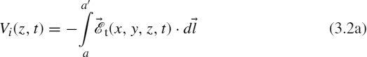
Figure 3.1 shows the general (n + 1)-conductor line to be considered. It consists of n conductors and a reference conductor (denoted as the zeroth conductor) to which the n line voltages will be referenced. This choice of the reference conductor is not unique. Applying Faraday's law to the contour c_i that encloses surface s_i shown between the reference conductor and the ith conductor gives

FIGURE 3.1 Illustration of the contour c_i and associated surface s_i for the derivation of the first transmission-line equation for the ith circuit.

where, again, denotes the transverse electric field (in the x–y cross-sectional plane) and denotes the longitudinal or z-directed electric field (along the surfaces of the conductors). Observe, once again, that because of the choice of the direction of the contour, the direction of (out of the page), and the right-hand rule, the minus sign on the right-hand side of Faraday's law is absent in (3.1). Once again, because of the assumption of a TEM field structure, we may uniquely define a voltage between the ith conductor and the reference conductor (positive on the ith conductor) as

We again define the per-unit-length conductor resistances as r_i Ω/m, and the per-unit-length resistance of the reference conductor is denoted as r₀ Ω/m. Thus,

The current of the ith conductor is

where the contour surrounds the ith conductor just off its surface. For the TEM field structure assumption it can be shown, as was the case for two-conductor lines, that the sum of the currents on all n + 1 conductors in the z direction at any cross section is zero. This is the basis for saying that the currents of the n conductors return through the reference conductor. Substituting into (1) yields

Dividing both sides by Δz and rearranging gives

Before taking the limit as Δz → 0, let us make some observations similar to the case of two-conductor lines. Clearly, the total magnetic flux penetrating the surface si in Figure 3.1 will be a linear combination of the fluxes due to the currents on all the conductors. Consider a cross-sectional view of the line looking in the direction of increasing z shown in Figure 3.2. The currents of the n conductors are implicitly defined in the positive z direction according to (3.4) since the contour surrounding the ith conductor is defined in the clockwise direction. Therefore, the magnetic fluxes due to the currents of the n conductors will also be in the clockwise direction looking in the direction of increasing z. The per-unit-length magnetic flux ψ_i penetrating the surface s_i between the reference conductor and the ith conductor is therefore defined to be in this clockwise direction when looking in the direction of increasing z as shown in Figure 3.2. Therefore, this per-unit-length magnetic flux penetrating surface si can be written as

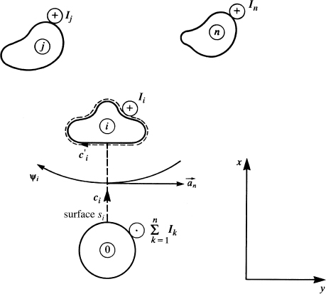
FIGURE 3.2 Cross-sectional illustration of the contour c_i and associated surface s_i for the derivation of the first transmission-line equation for the ith circuit.

Observe that a minus sign is again required in this flux expression. This is because the direction of the required flux, ψ_i, and the defined unit normal to the surface, , are in opposite directions. The l_ii term is the per-unit-length self-inductance of the ith circuit or loop, and the l_ij terms are the per-unit-length mutual inductances between this ith circuit and the jth circuit. Taking the limit of (3.6) as Δz → 0 and substituting (3.7) yields

This first MTL equation can be written in a compact form using matrix notation as

where the n × 1 voltage and current vectors are defined as

The per-unit-length inductance matrix is defined from (3.7) as

where ψ is an n × 1 vector containing the total magnetic fluxes per unit length, ψ_i, penetrating the ith circuit, which is the surface defined between the ith conductor and the reference conductor:

The flux through the circuit (loop), ψ_i, is directed in the clockwise direction when looking in the +z direction (see Figure 3.2). The per-unit-length inductance matrix L contains the individual per-unit-length self-inductances, l_ii, of the circuits and the per-unit-length mutual inductances between the circuits, l_ij. In Section 3.5, L will be shown to be a symmetric matrix as

Similarly, from (3.8) we define the per-unit-length resistance matrix as

Observe that this first transmission-line equation given in (3.9) is identical in form to the scalar first transmission-line equation for a two-conductor line given in (2.9) and (2.19) of Chapter 2.

This per-unit-length resistance matrix in (3.12) has a nice form but is restricted to reference conductors that are finite-sized conductors such as wires. In the case of a reference conductor being a large ground plane, each current returning in the ground plane will be concentrated beneath the “going down” conductor as illustrated in Figure 3.3. These currents spread out in the ground plane and cause the per-unit-length resistance matrix to be of the form

FIGURE 3.3 Illustration of “current spreading” in a ground plane and the principle that the return currents will concentrate beneath the associated “going-down” conductor.

where r_ij are due to the resistance of the ground plane and are generally not equal.

In order to derive the second MTL equation, we place a closed surface s′ around the ith conductor as shown in Figure 3.4. The portion of the surface over the end caps is denoted as , whereas the portion over the sides is denoted as . Recall the continuity equation or equation of conservation of charge:

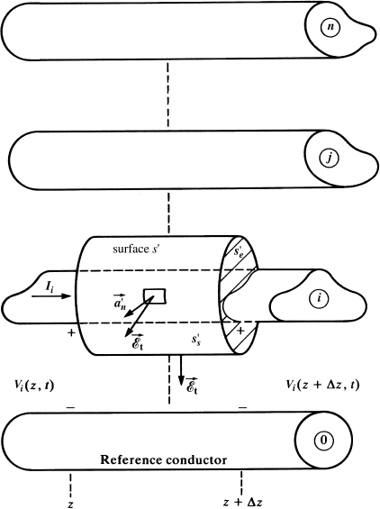
FIGURE 3.4 Illustration of the contour and associated surface for the derivation of the second transmission-line equation for the ith conductor.

Over the end caps, we have

Over the sides of the surface, there are again two currents: a conduction current , and displacement current , where the surrounding homogeneous medium is characterized by conductivity σ and permittivity ε. Again, these notions can be extended to an inhomogeneous medium surrounding the conductors in a similar manner. A portion of the left-hand side of (3.14) contains the transverse conduction current flowing between the conductors:

This can again be considered by defining per-unit-length conductances g_ij S/m between each pair of conductors as the ratio of conduction current flowing between the two conductors in the transverse plane to the voltage between the two conductors. Therefore, as illustrated in Figure 3.5(a),

Similarly, the charge enclosed by the surface (residing on the conductor surface) is, by Gauss' law,

The charge per unit of line length can be defined in terms of the per-unit-length capacitances c_ij between each pair of conductors. Therefore, as illustrated in Figure 3.5(a),

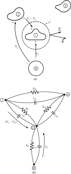
FIGURE 3.5 Cross-sectional illustration of (a) the contour and associated surface for the derivation of the second transmission-line equation for the ith conductor and (b) the equivalent per-unit-length conductances and capacitances.

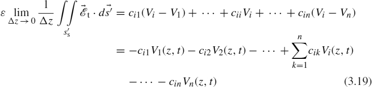
These concepts are illustrated in cross section in Figure 3.5(b). Substituting (3.15), (3.16), and (3.18) into (3.14) and dividing both sides by Δz gives

Taking the limit as Δz → 0 and substituting (3.17) and (3.19) yields

Equations (3.21) can be placed in compact form with matrix notation giving

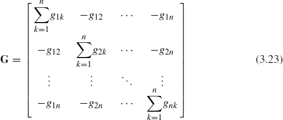
where V and I are defined by (3.10). The per-unit-length conductance matrix G represents the conduction current flowing between the conductors in the transverse plane and is defined from (3.17) as

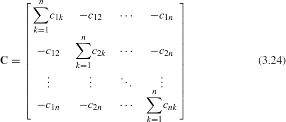
The per-unit-length capacitance matrix, C, represents the displacement current flowing between the conductors in the transverse plane and is defined from (3.19) as

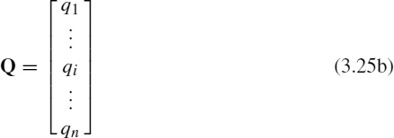
As will be shown in Section 3.5, both G and C are symmetric. Again observe that (3.22) is the matrix counterpart to the scalar second transmission-line equation for two-conductor lines given in (2.17) and (2.21) in Chapter 2. If we denote the total charge on the ith conductor per unit of line length as q_i, then the fundamental definition of C is

where Q is the n × 1 vector of the total per-unit-length charges

and V is given by (3.10a). Similarly, the fundamental definition of G is I_t = GV, where I_t is the n × 1 vector containing the transverse conduction currents between the conductors per unit of line length.

The above per-unit-length parameter matrices once again contain all the cross-sectional dimension information that distinguishes one MTL structure from another.

3.2 DERIVATION OF THE MULTICONDUCTOR TRANSMISSION-LINE EQUATIONS FROM THE PER-UNIT-LENGTH EQUIVALENT CIRCUIT

As an alternative method, we derive the MTL equations from the per-unit-length equivalent circuit shown in Figure 3.6. Writing Kirchhoff's voltage law around the ith circuit consisting of the ith conductor and the reference conductor yields

FIGURE 3.6 The per-unit-length equivalent circuit for derivation of the transmission-line equations.

Dividing both sides by Δz and taking the limit as Δz → 0 once again yields the first transmission-line equation given in (3.8) with the collection for all i given in matrix form in (3.9).

Similarly, the second MTL equation can be obtained by applying Kirchhoff's current law to the ith conductor in the per-unit-length equivalent circuit in Figure 3.6 to yield

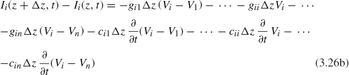
Dividing both sides by Δz, taking the limit as Δz → 0, and collecting terms once again yields the second transmission-line equation given in (3.21) with the collection for all i given in matrix form in (3.22).

3.3 SUMMARY OF THE MTL EQUATIONS

In summary, the MTL equations are given by the collection

The structures of the per-unit-length resistance matrix R in (3.12) or (3.13), inductance matrix L in (3.11c), conductance matrix G in (3.23), and capacitance matrix C in (3.24) are very important as are the definitions of the per-unit-length entries in those matrices. The precise definitions of these elements are rather intuitive and lead to many ways of computing them for a particular MTL type. These computational methods will be considered in detail in Chapters 4 and 5. The important properties of the per-unit-length parameter matrices will be obtained in Section 3.5. Again, these bear striking parallels to their scalar counterparts for the two-conductor line.

The MTL equations in (3.27) are a set of 2n, coupled, first-order, partial differential equations. They may be put in a more compact form as

We will find this first-order form to be especially helpful when we set out to solve them in later chapters. If the conductors are perfect conductors, then R = 0, whereas if the surrounding medium is lossless (σ = 0), then G = 0. The line is said to be lossless if both the conductors and the medium are lossless in which case the MTL equations simplify to

The first-order, coupled forms in (3.27) can be placed in the form of second-order, uncoupled equations by differentiating (3.27a) with respect to z and differentiating (3.27b) with respect to t to yield

In taking the derivatives with respect to z, we assume that the line is uniform; that is, the per-unit-length parameter matrices are independent of z. Substituting (3.30b) and (3.27b) into (3.30a) and reversing the process yields the uncoupled, second-order equations:

Observe that the various matrix products in (3.31) do not generally commute so that the proper order of multiplication must be observed.

3.4 INCORPORATING FREQUENCY-DEPENDENT LOSSES

We have so far neglected the important fact that, like the two-conductor case, the per-unit-length parameters in R, L, G, and C are generally frequency dependent, that is, R (ω), L (ω), G (ω), and C (ω). For perfect conductors, the currents reside on the surfaces of the conductors and R = 0. For imperfect conductors, the currents, because of skin effect, will migrate toward the conductor surfaces as frequency is increased, and at high frequencies will be concentrated near the conductor surfaces in annuli of thickness equal to a skin depth: . In addition, closely spaced conductors will cause the current distribution over the conductors to be nonuniformly distributed over the cross sections. The currents internal to the conductors will cause a per-unit-length internal inductance matrix L_i (ω) that is also frequency dependent. This is due to the magnetic flux internal to the conductors. As frequency increases, this internal flux decreases as a rate of eventually decreasing to zero. This internal inductance matrix can be included in the total inductance as the sum with the external inductance matrix that is due to the magnetic flux external to the conductors, L, which is substantially frequency independent. Similarly, the per-unit-length conductance matrix will be frequency dependent. This is because the dielectric will have a loss due to the incomplete alignment of the bound charges in it as frequency increases giving an effective conductivity that is frequency dependent, G (ω). Similarly, the relative permittivity of the surrounding dielectric is (mildly) dependent on frequency giving a (mildly) frequency-dependent per-unit-length capacitance matrix C (ω).

These frequency-dependent parameters can more readily be incorporated by writing the above MTL equations in the frequency domain by replacing in (3.27) to give

where and are the per-unit-length impedance and admittance matrices, respectively, and are given by

The second-order uncoupled equations are

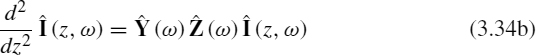
Again, the matrices do not generally commute and the proper order of multiplication must be preserved.

In the time domain, the frequency-domain MTL equations in (3.32) become

where * denotes convolution and the inverse Fourier transforms are denoted as

3.5 PROPERTIES OF THE PER-UNIT-LENGTH PARAMETER MATRICES L, C, G

In Chapter 1 we showed that, for a two-conductor line immersed in a homogeneous medium characterized by permeability μ, conductivity σ, and permittivity ε, the per-unit-length inductance l, conductance g, and capacitance c are related by lc = με and lg = μσ. For the case of an MTL consisting of n + 1 conductors immersed in a homogeneous medium characterized by permeability μ, conductivity σ, and permittivity ε, the per-unit-length parameter matrices are similarly related by

where the n × n identity matrix is defined as having unity entries on the main diagonal and zeros elsewhere:

Other important properties such as our logical assumption that these per-unit-length matrices are symmetric will also be shown.

Recall from Chapter 1 that the transverse electric and magnetic fields of the TEM field structure in a homogeneous medium characterized by ε, μ, and σ satisfy the following differential equations (see Eqs. (1.13) of Chapter 1):

Define voltage and current in the usual fashion as integrals in the transverse plane (see Fig. 2.3) as

Applying (3.40) to (3.39) yields

Collecting Eqs. (3.41) for all conductors in matrix form yields

Comparing (3.42) to (3.31) with R = 0 gives the identities in (3.37). Because of the identities in (3.37), which are valid only for a homogeneous medium, we need to determine only one of the per-unit-length parameter matrices since (3.37) can be written, for example, as

The previous relations in (3.37) and (3.43) are valid only for a homogeneous surrounding medium. In the remainder of this chapter, we will address the general case where the dielectric medium surrounding the n + 1 conductors may be inhomogeneous. Throughout this text, we will assume that any medium surrounding the line conductors (homogeneous or inhomogeneous) is not ferromagnetic and therefore has a permeability of free space, μ = μ₀. Designate the capacitance matrix with the surrounding medium (homogeneous or inhomogeneous) removed and replaced by free space having permeability ε₀ and permeability μ₀ as C₀. Since inductance depends on the permeability of the surrounding medium and does not depend on the permittivity of the medium, and the permeability of dielectrics is that of free space, μ₀, the inductance matrix L can be obtained from C₀ using the relations for a homogeneous medium (in this case, free space) given in (3.43a) as

Therefore, for an inhomogeneous medium, we may determine these per-unit-length parameter matrices by (1) computing the capacitance matrix with the inhomogeneous medium present, C, (2) computing the per-unit-length capacitance matrix with the inhomogeneous medium removed and replaced with free space, C₀, and then (3) computing L from (3.44). It turns out that we will also develop in Chapters 4 and 5 a method for computing G for an inhomogeneous medium from a modified capacitance calculation. Hence, we will only have to construct a capacitance solver in order to determine the per-unit-length parameter matrices of L, C, and G for the general case of an inhomogeneous medium. In Chapter 5, we will examine numerical methods for computing the entries in these per-unit-length matrices for an inhomogeneous medium surrounding the conductors.

The identities in (3.37) and (3.43) are valid only for a homogeneous surrounding medium as is the assumption of a TEM field structure and the resulting MTL equations. We will often extend the MTL equation representation, in an approximate manner, to include inhomogeneous media as well as imperfect conductors under the quasi-TEM assumption. In the case of a surrounding medium that is either homogeneous or inhomogeneous, the per-unit-length parameter matrices L, C, and G have several important properties. The primary ones are that they are symmetric and positive-definite matrices. As an illustration, we will prove that C is symmetric. The proof that C is a symmetric matrix (regardless of whether the surrounding medium is homogeneous or inhomogeneous) can be accomplished from energy considerations [A.1,1]. The basic relation for C is given in (3.25). Suppose we invert this relation to give

where P = C⁻¹ or, in expanded form,

If we can prove that p_ij = p_ji, then it follows that c_ij = c_ji. Suppose all conductors except the ith and jth are connected to the reference conductor (grounded) and all conductors are initially uncharged. Suppose we start charging the ith conductor to a final per-unit-length charge of q_i. Charging the ith conductor to an incremental charge q results in a voltage of the conductor, from (3.45b), of V_i = p_iiq. The incremental energy required to do this is dW = V_idq. The total energy required to place the charge q_i on the ith conductor is 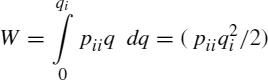. Now if we charge the jth conductor to an incremental charge of q in the presence of the charged ith conductor, the voltage of the jth conductor is V_j = p_jiq_i + p_jjq and the incremental energy required is dW = ( p_jiq_i + p_jjq)dq. The total energy required to charge the jth conductor to a charge of q_j becomes a. Thus, the total energy required to charge conductor i to q_i and conductor j to q_j is

If we reverse this process charging conductor j to q_j and then charging conductor i to q_i, we obtain

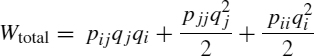
Since the total energies must be the same regardless of the sequence in which the conductors are charged, we see, by comparing these two energy expressions, that

Therefore, it follows that

and therefore the capacitance matrix C is symmetric.

Recall that this proof of symmetry relied on energy considerations and therefore is valid for inhomogeneous media. Because of the relation in (3.44), , it is clear that the per-unit-length inductance matrix is also symmetric. The proof that C, L, and G are symmetric matrices (regardless of whether the surrounding medium is homogeneous or inhomogeneous) can also be obtained from a more general relation called Green's reciprocity theorem [2]. This relation relies on the important assumption that the surrounding medium is isotropic. This means that the parameters of permittivity, permeability, and conductivity are scalars. An anisoptropic medium is one in which these parameters are matrices relating the three components of the vectors E, D, B, H, and J_t, where J_t is the vector of transverse currents flowing through the surrounding medium [A.1]. We also, of course, assume that the surrounding medium is linear.

We next set out to prove that L, C, and G are positive definite. The energy stored in the electric field per unit of line length is [2]

where the transpose of a matrix M is denoted by M^t. The vector Q contains the per-unit-length charges on the conductors and is given in (3.25b). Substituting the relation for C in (3.25a), Q = CV, into (3.46) gives

where we have used the matrix property that Q^t = [CV]^t = V^tC^t along with the previously proven property that C is symmetric, that is, C^t = C. This total energy stored in the electric field must be positive and nonzero for all nonzero choices of the voltages (positive or negative). Thus, we say that C is positive definite if

for all possible nonzero values of the entries in V. It turns out that this implies that all of the eigenvalues of C must be positive and nonzero, a property we will find very useful in our later developments [3].

Similarly, the energy stored in the magnetic field per unit of line length is [2]

where ψ is the n × 1 vector of magnetic fluxes through the respective circuits and is given in (3.11b). Substituting the relation for L given in (3.11a) gives

where ψ^t = [LI]^t = I^t L, and we use the property that L is symmetric, L^t = L. Since the stored magnetic energy must always be greater than zero, we see that L is positive definite also:

Again, this means that the eigenvalues of L are all positive and nonzero.

Matrices C and G have the unique property that the sum of all elements in any row is greater than zero (see (3.23) and (3.24)). Such a matrix is said to be hyperdominant. It can be shown that any hyperdominant matrix form is always positive definite (see Problem 3.11). Hence, G is also positive definite and therefore its eigenvalues are all positive and nonzero.

PROBLEMS

3.1 Demonstrate the result in (3.8).

3.2 Demonstrate the form of R given in (3.12).

3.3 Demonstrate the result in (3.21).

3.4 Demonstrate the form of G in (3.23).

3.5 Demonstrate the form of C in (3.24).

3.6 Derive the MTL equations for the per-unit-length equivalent circuit of a four-conductor line shown in Figure P3.6.

3.7 Demonstrate the result in (3.31).

3.8 A four-conductor line immersed in free space has the following per-unit-length inductance matrix:

3.9 Demonstrate the result in (3.42).

3.10 Show that the criterion for positive definiteness of a real, symmetric matrix is that its eigenvalues are all positive and nonzero. (Hint: Transform the matrix to another equivalent one with a transformation matrix that diagonalizes it as T⁻¹ MT = Λ, where Λ is diagonal with its eigenvalues on the main diagonal. It is always possible to diagonalize any real, symmetric matrix such that T⁻¹ = T^t, where T^t is the transpose of T.) Show that the per-unit-length inductance matrix in Problem 3.8 is positive definite.

3.11 A matrix with the structure of G in (3.23) or C in (3.24) whose off-diagonal terms are negative and the sum of the elements in a row or column is positive is said to be hyperdominant. Show that a hyperdominant matrix is always positive definite.

REFERENCES

[1] R.Plonsey and R.E. Collin, Principles and Applications of Electromagnetic Fields, 2nd edition, McGraw-Hill, New York, 1982.

[2] M. Javid and P.M. Brown, Field Analysis and Electromagnetics, McGraw-Hill, New York, 1963.

[3] F.E. Hohn, Elementary Matrix Algebra, 2nd edition, Macmillan, New York, 1964.