
6
FREQUENCY-DOMAIN ANALYSIS OF TWO-CONDUCTOR LINES
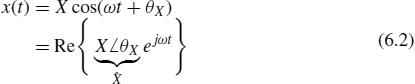
In this chapter, we will examine the solution of the transmission-line equations for two-conductor lines, where the line is excited by a single-frequency sinusoidal signal and is in steady state. The analysis method is the familiar phasor technique of electric circuit analysis [A.2, A.5]. The excitation sources for the line are single-frequency sinusoidal waveforms such as x(t) = Xcos (ωt + θX). Again, as explained in Chapter 1, the reason we invest so much time and interest in this form of line excitation is that we may decompose any other periodic waveform into an infinite sum of sinusoidal signals that have frequencies that are multiples of the basic repetition frequency of the signal via the Fourier series. We may then obtain the response to the original waveform as the superposition of the responses to those single-frequency harmonic components of the (nonsinusoidal) periodic input signal (see Figure 1.21 of Chapter 1). In the case of a nonperiodic waveform, we may similarly decompose the signal into a continuum of sinusoidal components via the Fourier transform and the analysis process remains unchanged. An additional reason for the importance of the frequency-domain method is that losses (of the conductors and the surrounding dielectric) can easily be handled in the frequency domain, whereas their inclusion in a time-domain analysis is problematic as we will see in Chapters 8 and 9. The per-unit-length resistance of the line conductors at high frequencies increases as the square root of the frequency, ![]() , because of skin effect, whereas the per-unit-length conductance of a homogeneous surrounding dielectric is also frequency dependent. In the frequency domain, we simply evaluate these at the frequency of interest and treat them as constants throughout the analysis.
, because of skin effect, whereas the per-unit-length conductance of a homogeneous surrounding dielectric is also frequency dependent. In the frequency domain, we simply evaluate these at the frequency of interest and treat them as constants throughout the analysis.
For the phasor method, we replace the excitation signal with its phasor equivalent as
where
We return to the time domain using Euler's identity by (1) multiplying the phasor result by ejωt and (2) taking the real part of the result:
6.1 THE TRANSMISSION-LINE EQUATIONS IN THE FREQUENCY DOMAIN
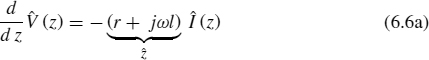
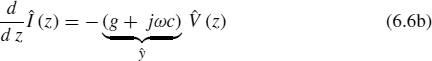
We form the phasor or frequency-domain differential equations by replacing all time derivatives with jω as
In the case of a lossless line, this reduces the time-domain partial differential transmission-line equations to their frequency-domain equivalent as
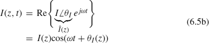
Observe that the frequency-domain or phasor transmission-line equations become ordinary differential equations because they are functions of only one variable, the line axis variable z. This is another important reason we go to the frequency domain: the solution of the transmission-line equations is simpler. Once we solve the phasor transmission-line ordinary differential equations in (6.4) and incorporate the terminal constraints at the left and right ends of the line, we return to the time domain by (1) multiplying the phasor solutions ![]() and Î(z) by ejωt and (2) taking the real part of that result as
and Î(z) by ejωt and (2) taking the real part of that result as

and
Losses of the line are incorporated via the per-unit-length resistance of the conductors, ![]() , and the per-unit-length conductance of the surrounding medium, g(f). The frequency-domain transmission-line equations in (6.4) are amended to
, and the per-unit-length conductance of the surrounding medium, g(f). The frequency-domain transmission-line equations in (6.4) are amended to
We will first examine the solution for a lossless line and then easily modify that solution for a lossy line.
6.2 THE GENERAL SOLUTION FOR LOSSLESS LINES
The transmission-line equations for a lossless line are given in (6.4) and repeated here:
These coupled first-order differential equations can be converted to uncoupled second-order differential equations in the usual manner by differentiating each with respect to z and substituting the other to yield (j2 = −1)
The general solution to these coupled second-order equations is again [A.1, A.6]
and
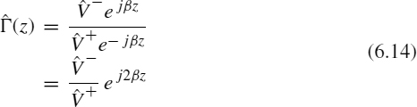
where the phase constant is again denoted as
and the phase velocity of propagation is
If the line is immersed in a homogeneous medium characterized by permittivity ε and permeability μ, then lc = με and ![]() . Hence, these TEM waves travel at the speed of light in that medium. The phase constant β represents a phase shift as the waves propagate along the line. The quantities
. Hence, these TEM waves travel at the speed of light in that medium. The phase constant β represents a phase shift as the waves propagate along the line. The quantities ![]() and
and ![]() are, as yet, undetermined constants. These will be determined by the specific load and source parameters. The line characteristic impedance is denoted as
are, as yet, undetermined constants. These will be determined by the specific load and source parameters. The line characteristic impedance is denoted as
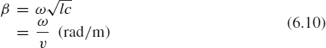
The source and load configurations at z = 0 and at z = ![]() are shown in Figure 6.1. In the frequency-domain representation, we may easily include inductors and capacitors in those complex-valued impedances,
are shown in Figure 6.1. In the frequency-domain representation, we may easily include inductors and capacitors in those complex-valued impedances, ![]() and
and ![]() . Once we incorporate the source and load terminal constraints into the general solution in (6.9) and determine the complex-valued constants
. Once we incorporate the source and load terminal constraints into the general solution in (6.9) and determine the complex-valued constants ![]() and
and ![]() , we can return to the time domain in the usual fashion by (1) multiplying the phasor result by ejωt and (2) taking the real part of the result to yield
, we can return to the time domain in the usual fashion by (1) multiplying the phasor result by ejωt and (2) taking the real part of the result to yield
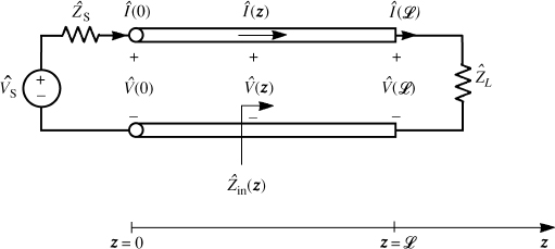
FIGURE 6.1 Definition of the parameters of a two-conductor line in the frequency domain.

and
where the undetermined constants are, in general, complex as ![]()
![]() . Observe that the characteristic impedance is the ratio of the voltage and current in the forward-traveling wave and the ratio of the voltage and current in the backward-traveling wave. Also, observe from (6.13) that since β = ω/v, we may write
. Observe that the characteristic impedance is the ratio of the voltage and current in the forward-traveling wave and the ratio of the voltage and current in the backward-traveling wave. Also, observe from (6.13) that since β = ω/v, we may write
![]()
This shows that the phase-shift term in the frequency-domain representation, e±jβz, is equivalent in the time domain to a time delay (t ± z/v).
6.2.1 The Reflection Coefficient and Input Impedance
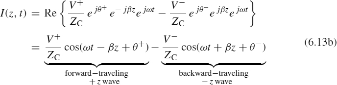
In order to incorporate the source and load into the general solution, we define a voltage reflection coefficient as the ratio of the (phasor) voltages in the backward-traveling and forward-traveling waves:
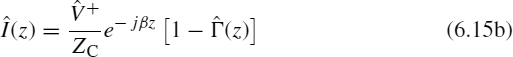
The general solution in (6.9) for the phasor voltage and current along the line can be written in terms of the reflection coefficient at that point by substituting (6.14):
Evaluating the general expression for the reflection coefficient anywhere along the line given in (6.14) at the load, z = ![]() , gives
, gives
At the load, the phasor voltage and current are related by Ohm's law as
Substituting (6.15) evaluated at the load, z = ![]() , gives
, gives

Solving this gives reflection coefficient at the load:

Substituting (6.16) into (6.14) gives an expression for the reflection coefficient at any point along the line in terms of the load reflection coefficient, which can be directly calculated via (6.19):
Substituting the explicit relation for the reflection coefficient in terms of the load reflection coefficient given in (6.20) into (6.15) gives a general expression for the phasor voltage and current anywhere on the line as
and
An important parameter of the line is the input impedance to the line at any point on the line. The input impedance is the ratio of the total voltage and current at that point as shown in Figure 6.1:

where we have substituted (6.15). The process for determining the input impedance is to (1) compute the load reflection coefficient from (6.19), (2) compute the reflection coefficient at the desired point from (6.20), and (3) then substitute that result into (6.22).
An important position to calculate the input impedance is at the input to the entire line, z = 0. The reflection coefficient at the input to the line is obtained from (6.20):
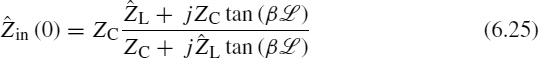
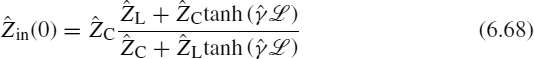
Hence, the input impedance to a line of length ![]() is
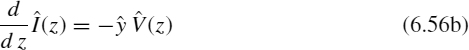
is
An explicit formula for this input impedance to the line can be obtained as [A.1, A.6]
A matched line is one in which the load impedance is equal to the characteristic impedance, ![]() . Hence, from (6.25) or (6.24) with
. Hence, from (6.25) or (6.24) with ![]() , the input impedance to a matched line is equal to the characteristic impedance at all points along the line and is purely resistive. Observe that for a lossless line the characteristic impedance
, the input impedance to a matched line is equal to the characteristic impedance at all points along the line and is purely resistive. Observe that for a lossless line the characteristic impedance ![]()
![]() is a real number. Hence, in order to match a lossless line the load impedance can only be purely resistive. A few other interesting facts may be observed from (6.25). Substituting β = 2π/λ, where the wavelength at the frequency of excitation of the line is λ = v/f, yields
is a real number. Hence, in order to match a lossless line the load impedance can only be purely resistive. A few other interesting facts may be observed from (6.25). Substituting β = 2π/λ, where the wavelength at the frequency of excitation of the line is λ = v/f, yields
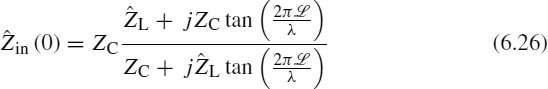
For a line that is one-quarter wavelength long, that is, ![]() = λ/4, (6.26) becomes
= λ/4, (6.26) becomes
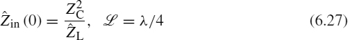
If the load is an open circuit, ![]() , then the input impedance to a quarter-wavelength section is a short circuit,
, then the input impedance to a quarter-wavelength section is a short circuit, ![]() . Conversely, if the load is a short circuit,
. Conversely, if the load is a short circuit, ![]() , then the input impedance to a quarter-wavelength section is an open circuit,
, then the input impedance to a quarter-wavelength section is an open circuit, ![]() . Also, (6.26) shows that for lengths of line that are a multiple of a half wavelength, that is,
. Also, (6.26) shows that for lengths of line that are a multiple of a half wavelength, that is, ![]() = n(λ/2) for n = 1, 2, 3,…, the input impedance replicates, that is,
= n(λ/2) for n = 1, 2, 3,…, the input impedance replicates, that is,
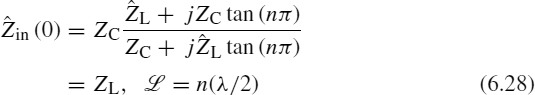
and
This result applies even if the line is not matched.
6.2.2 Solutions for the Terminal Voltages and Currents
In general, we will only be interested in determining the current and voltage at the input and output of the line. Evaluating (6.15) at z = 0 and z = ![]() gives
gives
and
If we can determine the undetermined constant ![]() , then we can determine the source and load voltages and currents by substituting into (6.30) and (6.31).
, then we can determine the source and load voltages and currents by substituting into (6.30) and (6.31).
In order to determine this undetermined constant, a convenient position to evaluate it is at the input to the line, z = 0. At the line input, the line can be replaced by the input impedance to the line as shown in Figure 6.2. The input voltage to the line can be determined by voltage division as

FIGURE 6.2 Determination of the phasor input voltage of the line.
Hence, the undetermined constant is determined from (6.30a) as

The process of determining the input and output voltages and currents to the line is
- Determine the load reflection coefficient
 from (6.19)
 - Determine the input reflection coefficient
 from (6.23)
 - Determine the input impedance to the line,
 , from (6.24) or (6.25)
 - Determine the input voltage
 from (6.32)
 - Determine the undetermined constant
 from (6.33)
 - Substitute this into (6.30) and (6.31) to determine the source and load voltages and currents.
A more direct way of determining these terminal voltages and currents is as follows. First, write the source relation in terms of a Thevenin equivalent relation as
Next, write the load terminal relation similarly as
Substitute the general solution in (6.9) evaluated at z = 0 and at z = ![]() into (6.34) and (6.35) to yield
into (6.34) and (6.35) to yield


Solve these two simultaneous equations for the two undetermined constants ![]() and
and ![]() and substitute them into the general solutions in (6.9) to determine the line voltage and current anywhere on the line and, in particular, at the source and the load. This general method of solution will be used in a virtually identical fashion for multiconductor transmission lines (MTLs) in the next chapter.
and substitute them into the general solutions in (6.9) to determine the line voltage and current anywhere on the line and, in particular, at the source and the load. This general method of solution will be used in a virtually identical fashion for multiconductor transmission lines (MTLs) in the next chapter.
For the simple case of a two-conductor line, (6.37) can be solved by hand in literal fashion (symbols instead of numbers) to give general expressions for ![]() and
and ![]() . These can then be written in closed form in terms of the reflection coefficients at the source and the load:
. These can then be written in closed form in terms of the reflection coefficients at the source and the load:

to give general expressions for the line voltage and current anywhere on the line as


A considerable amount of information can be gleaned from these informative expressions. For example, the source and load voltages and currents become

and


If the line is matched at the load, that is, ![]() , so that the load reflection coefficient is zero,
, so that the load reflection coefficient is zero, ![]() , these reduce to
, these reduce to


and


Observe that these results are sensible because the line input looks like ![]() , the magnitude of the voltage and current is constant all along the line, and the load and source voltage and current differ only by the phase shift of the line, e−jβ
, the magnitude of the voltage and current is constant all along the line, and the load and source voltage and current differ only by the phase shift of the line, e−jβ![]() .
.
6.2.3 The SPICE (PSPICE) Solution for Lossless Lines
SPICE (or PSPICE) can be used to solve these phasor transmission-line problems for lossless lines. The SPICE or its personal computer version, PSPICE, computer program contains a model that is an exact solution of the transmission-line equations for a lossless two-conductor transmission line. See Appendix B for a tutorial on the use of SPICE/PSPICE. This exact model will be derived in Chapter 8. It is invoked by the following statement:
TXXX N1 N2 N3 N4 Z0 = ZC TD = TD
where ![]() is the characteristic impedance of the line and TD = (
is the characteristic impedance of the line and TD = (![]() /v) is the one-way time delay for propagation from one end of the line to the other. The name of the element, TXXX, denotes the model and XXX is the name of that specific model given by the user. The line and model are connected between nodes N1–N2 and N3–N4 as shown in Figure 6.3. Normally, nodes N2 and N4 are chosen to be the universal reference or ground node, the zero node: N2 = 0 and N4 = 0.
/v) is the one-way time delay for propagation from one end of the line to the other. The name of the element, TXXX, denotes the model and XXX is the name of that specific model given by the user. The line and model are connected between nodes N1–N2 and N3–N4 as shown in Figure 6.3. Normally, nodes N2 and N4 are chosen to be the universal reference or ground node, the zero node: N2 = 0 and N4 = 0.
An example is shown in Figure 6.4(a). A 100-MHz voltage source having a magnitude of 10 V and an angle of 30° is attached to a two-conductor lossless line having a characteristic impedance of 50 Ω, a velocity of propagation of 200 m/μs, and a line length of 2.7 m. This gives a one-way time delay of TD = ![]() /v = 13.5 ns. The source impedance is
/v = 13.5 ns. The source impedance is ![]() and the load impedance is
and the load impedance is ![]() . The PSPICE node numbering is shown in Figure 6.4(b). SPICE requires R, L, and C circuit elements, so we have synthesized equivalent circuits for the source and load impedances as shown, which, at a frequency of 100 MHz, will give the desired complex impedances. The PSPICE program is
. The PSPICE node numbering is shown in Figure 6.4(b). SPICE requires R, L, and C circuit elements, so we have synthesized equivalent circuits for the source and load impedances as shown, which, at a frequency of 100 MHz, will give the desired complex impedances. The PSPICE program is

FIGURE 6.3 Representing a lossless transmission line with the SPICE (PSPICE) equivalent circuit.
EXAMPLE
VS 1 0 AC 10 30
RS 1 2 100
CS 2 3 31.8P
T 3 0 4 0 Z0=50 TD=13.5N
RL 4 5 100
LL 5 0 0.318U
.AC DEC 1 1E8 1E8
.PRINT AC VM(3) VP(3) VM(4) VP(4)
.END
The .AC command causes the program to calculate the result from a starting frequency of 100 MHz to an ending frequency of 100 MHz in steps of one frequency per decade. In other words, the solutions are obtained at only 100 MHz. The .PRINT statement requests that the results be printed to a file with the magnitude of the node voltage at node 3 denoted as VM(3) and the phase denoted as VP(3). The results are

and
![]()
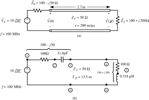
FIGURE 6.4 An example for computing the phasor terminal voltages of a lossless transmission line: (a) the problem statement and (b) the SPICE coding diagram.
These compare favorably with those computed directly by hand with the earlier results of
![]()
and
![]()
Observe that the load voltage angle of −409.12° is equivalent to −49.12°.
6.2.4 Voltage and Current as a Function of Position on the Line
We have been primarily interested in determining the voltages and currents at the endpoints of the line. In this section, we will investigate and provide plots of the magnitudes of the phasor line voltage and current at various points along the line. We will plot the magnitude of these for distances d = ![]() − z away from the load. Recall the expressions for the voltage and current at various positions along the line in (6.21). Substituting z =
− z away from the load. Recall the expressions for the voltage and current at various positions along the line in (6.21). Substituting z = ![]() − d into (6.21) and taking the magnitude gives
− d into (6.21) and taking the magnitude gives
There are three important cases of special interest that we will investigate: (1) the load is a short circuit, ![]() , (2) the load is an open circuit,
, (2) the load is an open circuit, ![]() , and (3) the load is matched,
, and (3) the load is matched, ![]() .
.
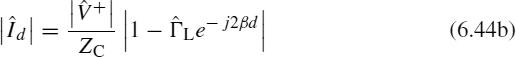
For the case where the load is a short circuit, ![]() , the load reflection coefficient is
, the load reflection coefficient is ![]() . Equations (6.44) reduce to
. Equations (6.44) reduce to
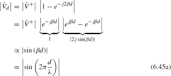
and
and we have written the result in terms of the distance from the load, d, in terms of wavelengths. These are plotted in Figure 6.5(b). Observe that the voltage is zero at the load and at distances from the load that are multiples of a half wavelength. The current is maximum at the load and is zero at distances from the load that are odd multiples of a quarter wavelength. Further, observe that corresponding points are separated by one-half wavelength. We will find this to be an important property for all other loads.
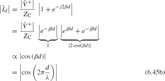
For the case where the load is an open circuit, ![]() , the load reflection coefficient is
, the load reflection coefficient is ![]() . Equations (6.44) reduce to
. Equations (6.44) reduce to
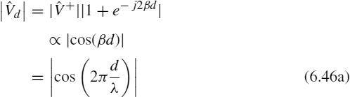
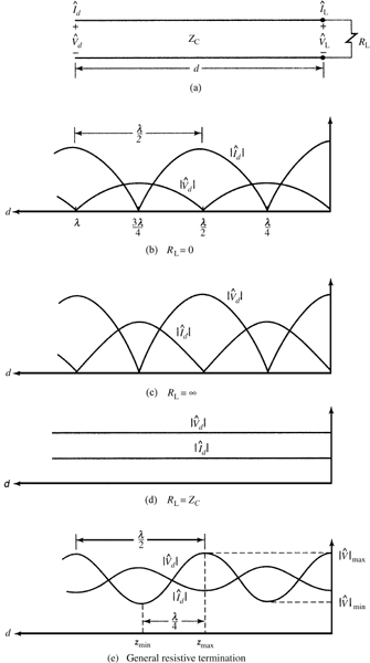
FIGURE 6.5 Illustration of the variation of the magnitudes of the line voltage and current for (b) a short-circuit load, RL = 0, (c) an open-circuit load, RL = ∞, (d) a matched load, RL = ZC and (e) a general resistive termination.

and we have again written the result in terms of the distance from the load, d, in terms of wavelengths. These are plotted in Figure 6.5(c). Observe that the current is zero at the load and at distances from the load that are multiples of a half wavelength. The voltage is maximum at the load and is zero at distances from the load that are odd multiples of a quarter wavelength. This is the reverse of the short-circuit load case. Further, again observe that corresponding points are separated by one-half wavelength.
And finally, we investigate the case of a matched load, ![]() . For this case, the load reflection coefficient is zero,
. For this case, the load reflection coefficient is zero, ![]() , so that the results in (6.44) show that the voltage and current are constant in magnitude along the line as shown in Figure 6.5(d). This is an important reason to match a line. Although the magnitudes of the voltage and current are constant along the line, they suffer a phase shift e−jβz as they propagate along it.
, so that the results in (6.44) show that the voltage and current are constant in magnitude along the line as shown in Figure 6.5(d). This is an important reason to match a line. Although the magnitudes of the voltage and current are constant along the line, they suffer a phase shift e−jβz as they propagate along it.
The general case is sketched in Figure 6.5(e). The locations of the voltage and current maxima and minima are determined by the actual load impedance, but adjacent corresponding points on each waveform are separated by one-half wavelength. This is an important and general result and can be proved from the general expressions in (6.44). In those expressions, the only dependence on the distance from the load, d, is in the phase term e−j2βd. Substituting β = 2π/λ and distances that are multiples of a half wavelength, d ![]() d ± n(λ/2), we obtain
d ± n(λ/2), we obtain
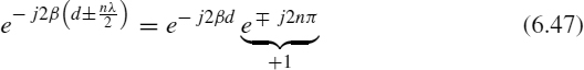
Hence, we obtain the important result that corresponding points on the magnitude of the line voltage and line current are separated by one-half wavelength in distance.
6.2.5 Matching and VSWR
Figure 6.5 illustrates how the magnitudes of the voltage and current vary with position on the line. In the matched case shown in Figure 6.5(d), the magnitudes of the voltage and current do not vary with position, but in the cases of a short-circuit or an open-circuit load (severely mismatched), the magnitudes of the voltage and current vary drastically with position achieving minima of zero. Observe that the maximum and the adjacent minimum are separated by one-quarter wavelength. This variation of the voltage and current along the line for a mismatched load is very undesirable as it can cause spots along the line where large voltages can occur that may damage insulation or produce load voltages and currents that are radically different from the input voltage to the line. Ideally, we would like the line to have no effect on the signal transmission (other than a phase shift or time delay) as will occur for the matched load.
Although we ideally always would like to match the line, there are many practical cases where we cannot exactly match the line. If ![]() , the line is mismatched but how do we quantitatively measure this degree of “mismatch”? A useful measure of this mismatch is the voltage standing wave ratio (VSWR). The VSWR is the ratio of the maximum voltage on the line to the minimum voltage on the line:
, the line is mismatched but how do we quantitatively measure this degree of “mismatch”? A useful measure of this mismatch is the voltage standing wave ratio (VSWR). The VSWR is the ratio of the maximum voltage on the line to the minimum voltage on the line:

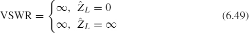
These maximum and minimum voltages will be separated by one-quarter wavelength. Observe that for the extreme cases of a short-circuit load, ![]() , or an open-circuit load,
, or an open-circuit load, ![]() , the minimum voltage is zero and hence the VSWR is infinite:
, the minimum voltage is zero and hence the VSWR is infinite:
but the VSWR is unity for a matched load:
The VSWR must therefore lie between these two bounds:
Industry considers a line to be “matched” if VSWR < 1.2
We can derive a quantitative result for the VSWR from (6.44a), which shows that the voltage at some distance d is proportional to ![]() . The maximum will be proportional to
. The maximum will be proportional to ![]() and the minimum will be proportional to
and the minimum will be proportional to ![]() . Hence, the VSWR is
. Hence, the VSWR is

6.2.6 Power Flow on a Lossless Line
We now investigate the power flow on a lossless line. The forward- and backward-traveling voltage and current waves carry power. The average power flowing to the right (+z) at a point on the line can be determined in terms of the total voltage and current at that point in the same fashion as for a lumped circuit as
where * denotes the complex conjugate. Substituting the general expressions for voltage and current given in (6.21) gives

and we have used the complex algebra result that the product of a complex number and its conjugate is the magnitude squared of that complex number. This result confirms that if the load is a short circuit, ![]() , or an open circuit,
, or an open circuit, ![]() , then the net power flow in the +z direction is zero. Clearly, an open circuit or a short circuit can absorb no power. Essentially, then the power in the forward-traveling wave is equal to the power in the backward-traveling wave and all the incident power is reflected.
, then the net power flow in the +z direction is zero. Clearly, an open circuit or a short circuit can absorb no power. Essentially, then the power in the forward-traveling wave is equal to the power in the backward-traveling wave and all the incident power is reflected.
This can be confirmed by separately computing the average power flow in the individual waves. The power flowing to the right in the forward-traveling wave is
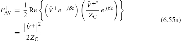
and the power flowing to the left in the backward-traveling wave is
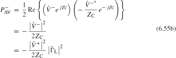
The sum of (6.55a) and (6.55b) gives (6.54). The ratio of reflected power to incident power is ![]() . For a matched load,
. For a matched load, ![]() ,
, ![]() and all the power in the forward-traveling wave is absorbed in the (matched) load.
and all the power in the forward-traveling wave is absorbed in the (matched) load.
6.3 THE GENERAL SOLUTION FOR LOSSY LINES
The transmission-line equations for lossy lines include the per-unit-length resistance of the conductors, ![]() , and the per-unit-length conductance of the lossy surrounding medium, g(f). The frequency-domain equations are
, and the per-unit-length conductance of the lossy surrounding medium, g(f). The frequency-domain equations are

where the per-unit-length impedance and admittance are
and
Differentiating one equation with respect to z and substituting the other, and vice versa, gives the uncoupled second-order differential equations

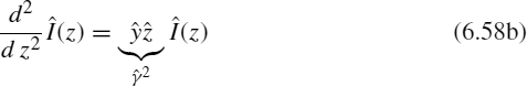
and the propagation constant is

The real part, α, is the attenuation constant and the imaginary part, β, is the phase constant. Observe that for a lossy line, ![]() , as was the case for the lossless line. Furthermore, the phase velocity of propagation along the line is
, as was the case for the lossless line. Furthermore, the phase velocity of propagation along the line is ![]() .
.
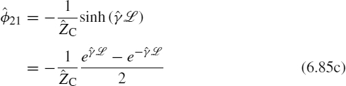
The general solution to (6.58) is [A.1]

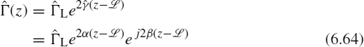
where the characteristic impedance now becomes complex as

The time-domain result is obtained in the usual fashion by (1) multiplying the phasor quantity by ejωt and (2) taking the real part of the result:
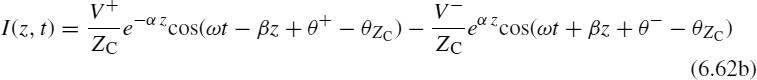
Again, the general solution consists of the sum of a forward-traveling wave (+z direction) and a backward-traveling wave (−z direction). Observe that there are only two differences between the lossless line solution and the lossy line solution. First, the voltage and current amplitudes are attenuated as shown by the terms e±αz. Second, the characteristic impedance is no longer real but has a phase angle. Hence, the voltage and current are no longer in time phase but are out of phase by θZC, which is at most 45°.
Hence, we can directly modify the results obtained for the lossless line to include losses by replacing jβ in those results with ![]() . For example, we define the load reflection coefficient as
. For example, we define the load reflection coefficient as

and the reflection coefficient anywhere on the line can be written in terms of the load reflection coefficient as
The phasor general solution in (6.60) becomes
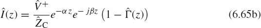
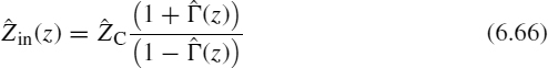
Hence, the input impedance of the line at a point along the line is the ratio of (6.65a) and (6.65b):
The input impedance to the entire line at z = 0 is
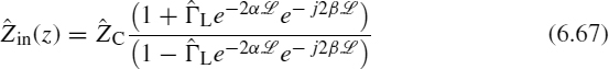
This can be written in an alternative form as
The solution process for determining the terminal voltages and currents of the line is virtually unchanged from the lossless case. The direct solution for the undetermined constants in (6.60) and given in (6.37) for the lossless case becomes

The explicit solution for the line voltage and current anywhere on the line given for the lossless line in (6.39) becomes for the lossy line


6.3.1 The Low-Loss Approximation
Typically, losses are small at the significant range of frequencies for typical high-speed digital signals and for typical boards. For example, for a stripline with plate separation of 20 mils and a land of width 5 mils in FR4 (εr = 4.7) we compute, from Eqs. (4.107) in Section 4.3.1 of Chapter 4, c = 113.2 pF/m and l = 0.461 μ H/m. The characteristic impedance for this lossless stripline is ![]() and the velocity of propagation is
and the velocity of propagation is ![]() . Using Eq. (4.60) of Chapter 4, the per-unit-length conductance is given by
. Using Eq. (4.60) of Chapter 4, the per-unit-length conductance is given by
where tan δ is the loss tangent of this (homogeneous) surrounding medium. For FR4 glass epoxy that is typical of PCBs, the loss tangent is approximately 0.02 in the low to high MHz range. Hence, for this board we obtain g = 14.2 × 10⁻¹² f S/m. The high-frequency resistance in (4.119) dominates the dc resistance in (4.118) above a frequency given in (4.120). For this problem and assuming that the constant k = 2, the frequency is 23 MHz. Hence, for frequencies above 23 MHz, the per-unit-length resistance of the land (thickness of 1.38 mils for 1 ounce copper) is computed from the high-frequency equation in (4.119) giving ![]() . By low loss we mean
. By low loss we mean
For this stripline problem, r is less than ωl for f > 1.34 MHz and g is less than ωc for all frequencies. Observe that since g = ω tan δc, g is less than ωc by the loss tangent, which for FR4 is on the order of 0.02 in the low to high MHz range. (The loss tangent goes to zero at dc and at very high frequencies.)
Let us consider obtaining a simple formula for the characteristic impedance and the attenuation constant. The propagation constant is given in (6.59). Rewriting this,
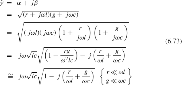
We now apply the Taylor's series to expand this:

to give
from which we identify the attenuation and phase constants as
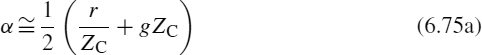
In a similar fashion, we obtain
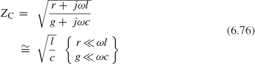
Hence for a low-loss line where ![]() and
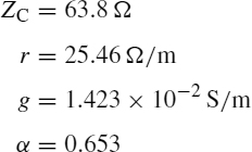
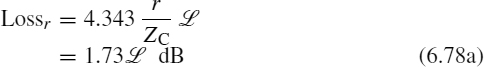
and ![]() , the characteristic impedance and the velocity of propagation are independent of frequency and are essentially the same as for a lossless line. Figure 6.6 shows the magnitude and angle of the characteristic impedance versus frequency from 10 kHz to 1 GHz for the stripline considered previously, where the land is of width 5 mils and the plate separation is 20 mils. Observe that above about 5 MHz the characteristic impedance approaches the lossless value of ZC = 63.8 Ω. Figure 6.7(a) shows the attenuation constant and Figure 6.7(b) shows the velocity of propagation, v = ω/β. The velocity of propagation approaches the lossless value of v = 1.38 × 10⁸m/s above about 5 MHz. The value of the attenuation constant computed from the approximation in (6.75a) at 100 MHz is α = 1.085 × 10⁻¹, whereas the value computed directly from the exact expression in (6.59) is the same. Hence for typical board dimensions, the low-loss region where the above approximations apply is above about 5 MHz. Hence for today's digital signals, all of their sinusoidal components lie in the low-loss frequency range.
, the characteristic impedance and the velocity of propagation are independent of frequency and are essentially the same as for a lossless line. Figure 6.6 shows the magnitude and angle of the characteristic impedance versus frequency from 10 kHz to 1 GHz for the stripline considered previously, where the land is of width 5 mils and the plate separation is 20 mils. Observe that above about 5 MHz the characteristic impedance approaches the lossless value of ZC = 63.8 Ω. Figure 6.7(a) shows the attenuation constant and Figure 6.7(b) shows the velocity of propagation, v = ω/β. The velocity of propagation approaches the lossless value of v = 1.38 × 10⁸m/s above about 5 MHz. The value of the attenuation constant computed from the approximation in (6.75a) at 100 MHz is α = 1.085 × 10⁻¹, whereas the value computed directly from the exact expression in (6.59) is the same. Hence for typical board dimensions, the low-loss region where the above approximations apply is above about 5 MHz. Hence for today's digital signals, all of their sinusoidal components lie in the low-loss frequency range.
Consider a lossy line that is matched so that there are only forward-traveling waves on the line. The voltage and current, according to (6.60), are attenuated according to e−αz as they travel along the line. Hence, the power loss in a line of length ![]() is e−2α
is e−2α![]() [A.1,A.3]. In dB, this becomes [A.3]
[A.1,A.3]. In dB, this becomes [A.3]
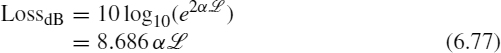
For the above stripline at a frequency of 1 GHz, we obtain
The resistive loss is
and the loss in the surrounding medium is

FIGURE 6.6 Plot of (a) the magnitude and (b) the phase of the line characteristic impedance for a low-loss line versus frequency.
FIGURE 6.7 Plot of (a) the attenuation constant and (b) the velocity of propagation for a low-loss line versus frequency.
The total loss is the sum of these. For a 6-in. length of this stripline, the total loss at 1 GHz is 0.86 dB. This says that the amplitude of a 1-GHz sine wave, which varies as e−αz, is reduced by about 1 dB; that is, the input level is reduced to about 90% at the output when traversing a line length of 6 in. Observe that above 1 GHz, the dielectric loss dominates the conductor loss.
6.4 LUMPED-CIRCUIT APPROXIMATE MODELS OF THE LINE
Although SPICE/PSPICE contains a model representing the exact solution of the transmission-line equations for a two-conductor lossless line, a frequently used alternative is a lumped-circuit approximate representation. The basic idea is to represent the line or segments of it as lumped circuits. Two common such models are the lumped-Pi and lumped-T models shown in Figure 6.8, named so for their topological appearance. In order for these to adequately represent the line, the line length must be electrically short at the excitation frequency; that is, ![]() < (1/10)λ. In some cases the line must be much shorter than this, electrically, say,
< (1/10)λ. In some cases the line must be much shorter than this, electrically, say, ![]() < (1/20)λ, in order for lumped-circuit models to characterize what is truly a distributed-parameter phenomenon. If the total line length exceeds this criterion, then it is divided into a sequence of smaller segments, each of which is electrically short. Observe that in each of these lumped circuits, the total capacitance is c
< (1/20)λ, in order for lumped-circuit models to characterize what is truly a distributed-parameter phenomenon. If the total line length exceeds this criterion, then it is divided into a sequence of smaller segments, each of which is electrically short. Observe that in each of these lumped circuits, the total capacitance is c![]() and the total inductance is l
and the total inductance is l![]() . For example, in the lumped-Pi circuit in Figure 6.8(b), the total line capacitance is split and put on either side of the total inductance. This gives the lumped circuit a reciprocal property that the actual line possesses. Similarly, the lumped-T model in Figure 6.8(c) has all the capacitance placed in the middle of the line, and the total inductance is split and placed on either side. This gives reciprocal structures.
. For example, in the lumped-Pi circuit in Figure 6.8(b), the total line capacitance is split and put on either side of the total inductance. This gives the lumped circuit a reciprocal property that the actual line possesses. Similarly, the lumped-T model in Figure 6.8(c) has all the capacitance placed in the middle of the line, and the total inductance is split and placed on either side. This gives reciprocal structures.

FIGURE 6.8 Illustration of lumped-circuit approximate models: (b) the lumped-Pi model and (c) the lumped-T model.
In order to investigate the adequacy of these approximate models, consider a two-conductor line of length 1 m and characterized by l = 0.5 μ H/m and c = 200pF/m shown in Figure 6.9(a). The characteristic impedance is 50 Ω and the velocity of propagation is 1 × 10⁸ m/s, giving a one-way time delay of 10 ns. The node numbering for the exact transmission-line model representation is shown in Figure 6.9(a). Figure 6.9(b) shows a one-section lumped-Pi model of the line along with the PSPICE node numbering. Figure 6.9(c) shows the line being broken in half and modeled with two lumped-Pi sections along with the PSPICE node numbering. The line is λ/10 at 10 MHz. Combining these three models into one program using one voltage source gives

FIGURE 6.9 SPICE simulation of the frequency-response of (a) the transmission-line model, (b) a one-section lumped-Pi model, and (c) a two-section lumped-Pi model.
EXAMPLE
    VS 1 0 AC 1
*   TRANSMISSION LINE MODEL
    RS1 1 2 10
    T 2 0 3 0 Z0=50 TD=10N
    RL1 3 4 100
    LL1 4 0 0.2653U
*   ONE-PI SECTION
    RS2 1 5 10
    C11 5 0 100P
    L11 5 6 0.5U
    C12 6 0 100P
    RL2 6 7 100
    LL2 7 0 0.2653U
*   TWO-PI SECTIONS
    RS3 1 8 10
    C21 8 0 50P
    L21 8 9 0.25U
    C22 9 0 50P
    C23 9 0 50P
    L22 9 10 0.25U
    C24 10 0 50P
    RL3 10 11 100
    LL3 11 0 0.2653U
    .AC DEC 50 1E6 100E6
    .PRINT AC VM(2) VP(2) VM(3) VP(3) VM(5) VP(5)
+       VM(6) VP(6) VM(8) VP(8) VM(10) VP(10)
    .PROBE
    .END
Plots of the input and output voltages of the line resulting from these three models are shown in Figure 6.10. Observe that for frequencies below where the line is λ/10, that is, 10 MHz, all three models give the same result. The lumped-Pi model consisting of two sections extends this prediction range slightly higher. Previous work has shown that increasing the number of sections does not significantly increase the prediction range of the lumped-circuit model to make the increased complexity of the circuit worth it [B.15].

FIGURE 6.10 Plots of the SPICE-computed magnitudes of the circuits of Figure 6.9 for (a) the source voltages and (b) the load voltages.
Lossy lines can also be modeled with these lumped-circuit approximations. The line can similarly be modeled with lumped-Pi or lumped-T sections but with the line per-unit-length resistance and conductance added as shown in Figure 6.11. Again, observe that the totals are r![]() and g
and g![]() . However, these per-unit-length parameters of resistance and conductance are frequency dependent as discussed in Sections 4.2.3 and 4.3.2 of Chapter 4. In the case of lossy lines excited at one frequency, these approximate models have a useful role since these per-unit-length parameters can be evaluated at the frequency of excitation and included in these models as a constant value element. However, in modeling time-domain excitation of the line such as the line driven by digital pulse waveforms, there is a significant problem. The digital pulse waveforms contain a continuum of sinusoidal components. Yet the per-unit-length resistance and conductance are frequency dependent. Hence, we should not use these lumped-circuit approximate models to model lines that are excited by general waveforms unless we ignore the frequency-dependant losses.
. However, these per-unit-length parameters of resistance and conductance are frequency dependent as discussed in Sections 4.2.3 and 4.3.2 of Chapter 4. In the case of lossy lines excited at one frequency, these approximate models have a useful role since these per-unit-length parameters can be evaluated at the frequency of excitation and included in these models as a constant value element. However, in modeling time-domain excitation of the line such as the line driven by digital pulse waveforms, there is a significant problem. The digital pulse waveforms contain a continuum of sinusoidal components. Yet the per-unit-length resistance and conductance are frequency dependent. Hence, we should not use these lumped-circuit approximate models to model lines that are excited by general waveforms unless we ignore the frequency-dependant losses.
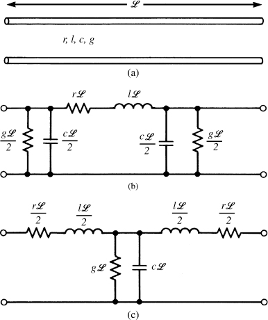
FIGURE 6.11 Illustration of the inclusion of losses into (b) the lumped-Pi and (c) the lumped-T equivalent circuits.
6.5 ALTERNATIVE TWO-PORT REPRESENTATIONS OF THE LINE
Since we are generally not interested in the line voltages and currents at points along the line other than at the terminations, we can imbed the line as a two-port as shown in Figure 6.12 and relate the terminal voltages and currents with two-port parameters.
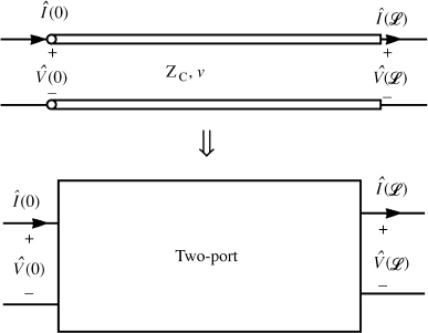
FIGURE 6.12 Characterization of a transmission line as a two-port.
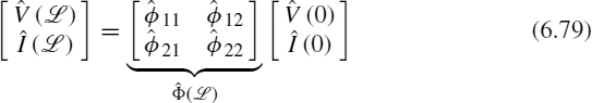
6.5.1 The Chain Parameters
One of the most useful forms of two-port parameters for a transmission line is the chain-parameter matrix representation. This relates the terminal voltages and currents as
These can be straightforwardly obtained by evaluating the general solutions for a lossless line given in (6.9) at z = 0 and z = ![]() to give
to give


Inverting (6.80a) gives
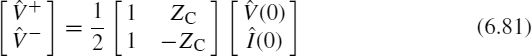
Substituting this into (6.80b) gives
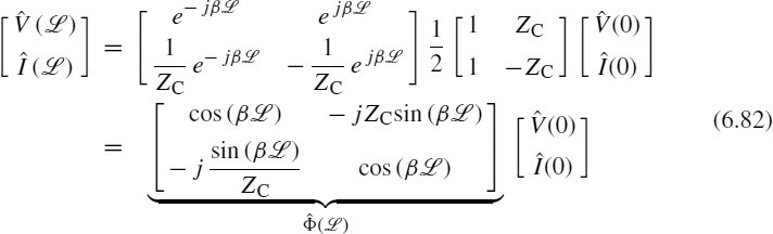
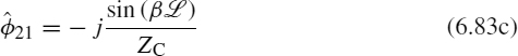
Hence, for a lossless line the chain parameters are
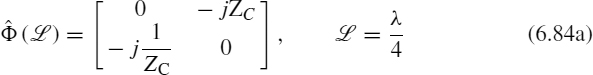
Observe some interesting properties of the chain-parameter matrix for a lossless line. If the line length is one quarter of a wavelength, β![]() = 2π(
= 2π(![]() / λ) = π/2 and the chain-parameter matrix becomes
/ λ) = π/2 and the chain-parameter matrix becomes
Conversely, if the line length is one-half wavelength, the chain-parameter matrix becomes

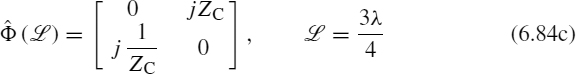
If the line length is three quarters of a wavelength, the chain-parameter matrix becomes
If the line is one wavelength, the chain-parameter matrix becomes the identity matrix:

which means that the input and output voltages are equal as are the input and output currents.
These are obtained for a lossless line. To obtain the chain parameters for a lossy line, we simply replace ![]() and replace
and replace ![]() along with
along with ![]() . Hence, for a lossy line, the chain parameters become
. Hence, for a lossy line, the chain parameters become


The chain parameters only relate the voltage and current at one end of the line to the voltage and current at the other end of the line. They do not explicitly determine those voltages and currents until we incorporate the terminals conditions. In order to incorporate the terminal conditions, we write the terminal conditions in the form of Thevenin equivalents. For example, for the typical terminations shown in Figure 6.1, these become
and
Writing out the chain-parameter representation in (6.79) and substituting (6.86) gives
Substituting (6.87b) into (6.87a) yields.
and
Once (6.88a) is solved for the current at z = 0, (6.88b) can be solved for the current at z = ![]() . Then the voltages can be obtained from the terminal relations in (6.86).
. Then the voltages can be obtained from the terminal relations in (6.86).
6.5.2 Approximating Abruptly Nonuniform Lines with the Chain-Parameter Matrix
The chain-parameter matrix relates the voltage and current at the right end of the line to the voltage and current at the left end of the line. Hence, the overall chain-parameter matrix of several such lines that are cascaded in series can be obtained as the product of the chain-parameter matrices of the sections (in the proper order). For example, consider the cascade of N lines or sections of lines having chain-parameter matrices Φ (Δ zi), each of length Δ zi for i = 1, 2, 3,…,N as shown in Figure 6.13(a). In other words, the overall chain-parameter matrix is
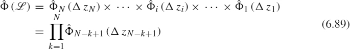
It is important to observe the proper order of multiplication of the individual chain-parameter matrices in this product. This is a result of the definition of the chain-parameter matrices as

and

Figure 6.13(b) and (c) shows that the chain-parameter representation can be used to model nonuniform lines. For example, the twisted pair of wires shown in Figure 6.13(b) is truly a bifilar helix, but we can approximate it as a sequence of loops lying in the page with an abrupt interchange at the junctions. The chain-parameter matrices of the uniform sections are then multiplied together along with chain-parameter matrices that give an interchange of the voltages and currents at the junctions. If the lengths of the sections are assumed to be identical, then the overall chain-parameter matrix is the Nth power of the chain-parameter matrix of each section (that includes the interchange chain-parameter matrix). This can be computed quite efficiently using, for example, the Cayley–Hamilton theorem for powers of a matrix [A.2, G.1, G.6, G.7].
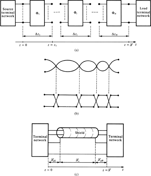
FIGURE 6.13 Representing abruptly nonuniform lines as (a) a cascade of uniform subsections, and applications to (b) twisted pairs and (c) shielded wires with pigtails.
Figure 6.13(c) shows another application for shielded cables. Shielded cables often have exposed sections at the ends to facilitate connection of the shield to the terminal networks [F.1–F.6]. The shield is connected to the terminations via a “pigtail” wire over the exposed sections. The overall chain-parameter matrix can then be obtained as the product of the chain-parameter matrices for the pigtail sections of length ![]() pL and
pL and ![]() pR and the chain-parameter matrix of the shielded section of length
pR and the chain-parameter matrix of the shielded section of length ![]() S as
S as
Once the overall chain-parameter matrix is obtained, the terminal constraints at the left and right ends of the line can be incorporated to solve for the terminal voltages and currents as described previously.
6.5.3 The Z and Y Parameters
The Z (impedance) parameters have the units of ohms and relate the voltages to the currents. These are defined as
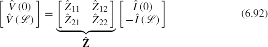
For the Z and Y parameters, the currents are defined to be directed into the two-port. Hence, we use −Î(![]() ) in this matrix representation. For a lossless line, the impedance parameters are again obtained by eliminating
) in this matrix representation. For a lossless line, the impedance parameters are again obtained by eliminating ![]() and
and ![]() from the basic solution in (6.9) to yield
from the basic solution in (6.9) to yield

The Z-parameter matrix is symmetric, so we may write it as

where

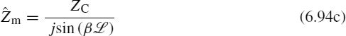
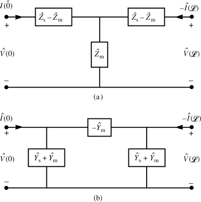
FIGURE 6.14 Equivalent circuits for (a) the Z parameters and (b) the Y parameters.
An (exact) equivalent circuit for the Z-parameter representation is shown in Figure 6.14(a).
Similarly, the Y (admittance) parameters relate the terminal currents to the terminal voltages and have the units of siemens and are defined as
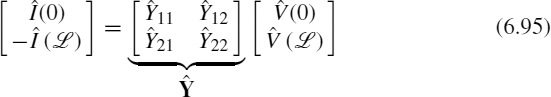
The Y-parameter matrix is the inverse of the Z-parameter matrix, Y = Z−1, so that
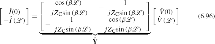
The Y-parameter matrix is symmetric, so we may write it as
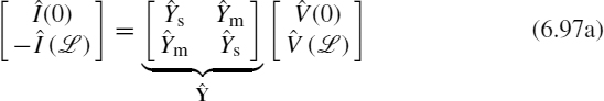
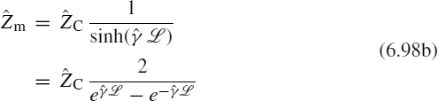
An (exact) equivalent circuit for the Y-parameter representation is shown in Figure 6.14(b). Observe that the Z-and Y-parameter matrices are singular when the line length is a multiple of a half wavelength, that is, ![]() = n(λ/2), because sin(β
= n(λ/2), because sin(β![]() ) = sin(2π(
) = sin(2π(![]() /λ)) is zero. The chain-parameter matrix on the contrary is never singular.
/λ)) is zero. The chain-parameter matrix on the contrary is never singular.
These are obtained for a lossless line. To obtain the Z or Y parameters for a lossy line, we again simply replace ![]() and replace
and replace ![]() along with
along with ![]() . Hence, for a lossy line the Z parameters become
. Hence, for a lossy line the Z parameters become
and the Y parameters become
and  .
.
As was the case for the chain parameters, the Z and Y parameters only relate the voltages at each end of the line to the currents at each end of the line; they do not explicitly determine them. As was the case for the chain parameters, the terminal conditions in (6.86) can be combined with the Z or Y parameters to give equations to explicitly solve for the terminal voltages and currents.
PROBLEMS
6.1 Show by direct substitution that (6.9) satisfy (6.8).
6.2 Show that (6.25) and (6.24) are equivalent.
6.3 For the transmission line shown in Figure 6.1, f = 5 MHz, v = 3 × 10⁸m/s, ![]() = 78 m, ZC = 50 Ω,
= 78 m, ZC = 50 Ω, ![]() ,
, ![]() ,
, ![]()
![]() . Determine (a) the line length as a fraction of a wavelength, (b) the voltage reflection coefficient at the load and at the input to the line, (c) the input impedance to the line, (d) the time-domain voltages at the input to the line and at the load, (e) the average power delivered to the load, and (f) the VSWR. [(a) 1.3, (b)
. Determine (a) the line length as a fraction of a wavelength, (b) the voltage reflection coefficient at the load and at the input to the line, (c) the input impedance to the line, (d) the time-domain voltages at the input to the line and at the load, (e) the average power delivered to the load, and (f) the VSWR. [(a) 1.3, (b) ![]() ,
, ![]() , (c)
, (c) ![]() , (d) 20.55cos(10π × 106t + 121.3°), 89.6cos(10π × 106t − 50.45°), (e) 2.77 W, and (f) 29.21]
, (d) 20.55cos(10π × 106t + 121.3°), 89.6cos(10π × 106t − 50.45°), (e) 2.77 W, and (f) 29.21]
6.4 For the transmission line shown in Figure 6.1, f = 200 MHz, v = 3 × 10⁸m/s, ![]() = 2.1m, ZC = 100 Ω,
= 2.1m, ZC = 100 Ω, ![]() ,
, ![]() , and
, and ![]() . Determine (a) the line length as a fraction of a wavelength, (b) the voltage reflection coefficient at the load and at the input to the line, (c) the input impedance to the line, (d) the time-domain voltages at the input to the line and at the load, (e) the average power delivered to the load, and (f) the VSWR. [(a) 1.4, (b)
. Determine (a) the line length as a fraction of a wavelength, (b) the voltage reflection coefficient at the load and at the input to the line, (c) the input impedance to the line, (d) the time-domain voltages at the input to the line and at the load, (e) the average power delivered to the load, and (f) the VSWR. [(a) 1.4, (b) ![]() ,
, ![]() , (c)
, (c) ![]() , (d) 9.25cos(4π × 108t + 46.33°), 4.738cos(4π × 108t − 127°), (e) 43 mW, and (f) 12.52]
, (d) 9.25cos(4π × 108t + 46.33°), 4.738cos(4π × 108t − 127°), (e) 43 mW, and (f) 12.52]
6.5 For the transmission line shown in Figure 6.1, f = 1G Hz, v = 1.7 × 10⁸m/s, ![]() = 11.9 cm, ZC = 100 Ω,
= 11.9 cm, ZC = 100 Ω, ![]() ,
, ![]() , and
, and ![]() . Determine (a) the line length as a fraction of a wavelength, (b) the voltage reflection coefficient at the load and at the input to the line, (c) the input impedance to the line, (d) the time-domain voltages at the input to the line and at the load, (e) the average power delivered to the load, and (f) the VSWR. [(a) 0.7, (b)
. Determine (a) the line length as a fraction of a wavelength, (b) the voltage reflection coefficient at the load and at the input to the line, (c) the input impedance to the line, (d) the time-domain voltages at the input to the line and at the load, (e) the average power delivered to the load, and (f) the VSWR. [(a) 0.7, (b) ![]() ,
, ![]() , (c)
, (c) ![]() , (d) 3.901cos(2π × 109t + 38.72°), 13.67cos(2π × 109t + 38.72°), (e) 0 W, and (f) ∞]
, (d) 3.901cos(2π × 109t + 38.72°), 13.67cos(2π × 109t + 38.72°), (e) 0 W, and (f) ∞]
6.6 For the transmission line shown in Figure 6.1, f = 600 MHz, v = 2 × 10⁸m/s, ![]() = 53 cm, ZC = 75 Ω,
= 53 cm, ZC = 75 Ω,![]() ,
, ![]() and
and ![]() . Determine (a) the line length as a fraction of a wavelength, (b) the voltage reflection coefficient at the input to the line and at the load, (c) the input impedance to the line, (d) the time-domain voltages at the input to the line and at the load, (e) the average power delivered to the load, and (f) the VSWR. [(a) 1.59, (b)
. Determine (a) the line length as a fraction of a wavelength, (b) the voltage reflection coefficient at the input to the line and at the load, (c) the input impedance to the line, (d) the time-domain voltages at the input to the line and at the load, (e) the average power delivered to the load, and (f) the VSWR. [(a) 1.59, (b) ![]() ,
, ![]() , (c)
, (c) ![]() , (d) 17.71cos(12π × 108t + 19.37°), 24.43cos(12π × 106t − 163.8°), (e) 0.298 W, and (f) 14.02]
, (d) 17.71cos(12π × 108t + 19.37°), 24.43cos(12π × 106t − 163.8°), (e) 0.298 W, and (f) 14.02]
6.7 For the transmission line shown in Figure 6.1, f = 1 MHz, v = 3 × 10⁸m/s, ![]() = 108 m, ZC = 300 Ω,
= 108 m, ZC = 300 Ω, ![]() ,
, ![]() , and
, and ![]()
![]() . Determine (a) the line length as a fraction of a wavelength, (b) the voltage reflection coefficient at the load and at the input to the line, (c) the input impedance to the line, (d) the time-domain voltages at the input to the line and at the load, (e) the average power delivered to the load, and (f) the VSWR. [(a) 0.36, (b)
. Determine (a) the line length as a fraction of a wavelength, (b) the voltage reflection coefficient at the load and at the input to the line, (c) the input impedance to the line, (d) the time-domain voltages at the input to the line and at the load, (e) the average power delivered to the load, and (f) the VSWR. [(a) 0.36, (b) ![]() ,
, ![]() , (c)
, (c) ![]() , (d) 99.2cos(2π × 106t − 6.127°), 46.5cos(2π × 106t − 153.3°), (e) 5.41 W, and (f) 3.37]
, (d) 99.2cos(2π × 106t − 6.127°), 46.5cos(2π × 106t − 153.3°), (e) 5.41 W, and (f) 3.37]
6.8 Confirm the input and load voltages for Problem 6.3 using SPICE.
6.9 Confirm the input and load voltages for Problem 6.4 using SPICE.
6.10 Confirm the input and load voltages for Problem 6.5 using SPICE.
6.11 Confirm the input and load voltages for Problem 6.6 using SPICE.
6.12 Confirm the input and load voltages for Problem 6.7 using SPICE.
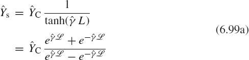
6.13 A half-wavelength dipole antenna is connected to a 100-MHz source with a 3.6-m length of 300-Ω transmission line (twin lead, v = 2.6 × 10⁸m/s) as shown in Figure P6.13. The source is represented by an open-circuit voltage of 10 V and source impedance of 50 Ω, whereas the input to the dipole antenna is represented by a 73-Ω resistance in series with an inductive reactance of 42.5 Ω. The average power dissipated in the 73-Ω resistance is equal to the power radiated into space by the antenna. Determine the average power radiated by the antenna with and without the transmission line and the VSWR on the line. [91.14 mW, 215.53 mW, 4.2]
FIGURE P 6.13
6.14 Two identical half-wavelength dipole antennas are connected in parallel and fed from one 300-MHz source as shown in Figure P6.14. Determine the average power delivered to each antenna. Hint: Determine the electrical lengths of the transmission lines. [115 mW]
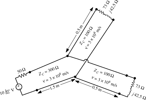
FIGURE P 6.14
6.15 Demonstrate the incorporation of terminal impedances in (6.37).
6.16 Demonstrate the formula for the voltage and current anywhere on the line in (6.39).
6.17 Demonstrate the power flow relation in (6.54).
6.18 Show, by direct substitution, that (6.60) satisfies (6.58).
6.19 Demonstrate the results in (6.75).
6.20 A low-loss coaxial cable has the following parameters: ![]() , α = 0.05, and v = 2 × 10⁸m/s. Determine the input impedance to a 11.175-m length of the cable at 400 MHz if the line is terminated in (a) a short circuit, (b) an open circuit, and (c) a 300-Ω resistor. [(a)
, α = 0.05, and v = 2 × 10⁸m/s. Determine the input impedance to a 11.175-m length of the cable at 400 MHz if the line is terminated in (a) a short circuit, (b) an open circuit, and (c) a 300-Ω resistor. [(a) ![]() , (b)
, (b) ![]() , and (c) 66.7/21.2° Ω]
, and (c) 66.7/21.2° Ω]
6.21 An air-filled line (v = 3 × 10⁸m/s) having a characteristic impedance of 50 Ω is driven at a frequency of 30 MHz and is 1 m in length. The line is terminated in a load of ![]() . Determine the input impedance using (a) the transmission-line model and (b) the approximate lumped-Pi model. Use PSPICE to compute both results. [(a) (12.89 − j51.49) Ω, and (b) (13.76 − j52.25) Ω]
. Determine the input impedance using (a) the transmission-line model and (b) the approximate lumped-Pi model. Use PSPICE to compute both results. [(a) (12.89 − j51.49) Ω, and (b) (13.76 − j52.25) Ω]
6.22 A lossless coaxial cable (v = 2 × 10⁸m/s) having a characteristic impedance of 100 Ω is driven at a frequency of 4 MHz and is 5 m in length. The line is terminated in a load of ![]() and the source is
and the source is ![]() with
with ![]() . Determine the input and output voltages to the line using (a) the transmission-line model, and (b) the approximate lumped-Pi model. Use PSPICE to compute both results. [Exact:
. Determine the input and output voltages to the line using (a) the transmission-line model, and (b) the approximate lumped-Pi model. Use PSPICE to compute both results. [Exact: ![]() ,
, ![]()
![]() ; approximate:
; approximate: ![]() ,
, ![]()
![]() ]
]
6.23 Verify the chain-parameter relations in (6.82).
6.24 Verify the Z parameters in (6.93).
6.25 Verify the Y parameters in (6.96).
6.26 Verify the equivalent circuits for the Z and Y parameters in Figure 6.14.