2.1 Communication protocol

As shown in Fig. 3, each local box contains controlling, monitoring, and communication hardware. All local boxes are in a mesh arrangement network facilitated by the XBee communication protocol. Each local box representing a node communicates with other nodes in this model. The advantage of a mesh network is its reliability; that is, if the communication between a pair of nodes is not working, the data can be transmitted through other nodes.

This protocol was chosen because of its short-range wireless data transmission technology, which is safe, reliable, simple, flexible, and low cost with a long battery life. The XBee module, shown in Fig. 4, is an interoperable RF module that establishes a mesh network in which all nodes need to have Zigbee as the transmitter terminal. Improved data traffic management, remote firmware updates, and self-healing and discovery for network stability capability make the Zigbee communication protocol exceptional among other protocols. In the smart community, the communication between the houses is established using the XBee communication protocol because there is clear distance between nodes.

2.2 System hardware configuration

As presented in Fig. 5, the Galvin Center Smart Home model is divided into different controllability areas facilitated by local control panels.

Each of the Smart Home area's local box, shown in Fig. 5, includes the office and garage area, the bathroom and bedroom, and the kitchen and living room. It contains numbers of current sensors and relay switches for each load and one XBee and microcontroller for each local box, as shown in Fig. 6. Lighting and HVAC systems are normally scheduled based on the optimization result and historical data. Motion and daylight sensors are used if some irregular occupancy or climate situation occurs.

This system monitors and controls all the Smart Home prototype electrical loads. In this model, all electrical loads are categorized into three different groups, including:

1. (1) adjustable loads such as HVAC, lighting, and the refrigerator with energy consumption levels that can be partially curtailed/increased due to the control signal.
2. (2) shiftable loads such as the dishwasher, washer, dryer, electrical pool pump, and plug-in hybrid vehicle (PHEV) with energy consumption levels that are considered as a load block with a constant rated power and known duty cycle. They would be on/off at the time the price of electricity is low/high and continue until its operation is completed.
3. (3) fixed loads such as microwaves, TVs, and computers with energy consumption levels that cannot be changed except by the tenant. Each load's real-time energy consumption can be measured dynamically every 1 s. These data are stored in the system database as historical data and are reprocessed for a self-learning operation. The database was created using the Microsoft SQL server. The controlling signal is sent to each appliance's circuit breaker initiated from the HEMS processor and can be transferred through the XBee communication protocol-based cloud within the Smart Home model.

2.3 System software configuration

Remote monitoring and scheduling of energy consumption is the main capability of this system. Smart Home tenants can monitor real-time energy consumption for specific areas and appliances and submit the schedule remotely through their portable devices. The controlling and monitoring dashboard engine, shown in Fig. 7, is a cloud-based application and enables the tenants to have access to the database and to control the electrical loads through remotely controllable circuit breakers. Each user can visualize the real-time data, including electrical load real-time energy consumption, circuit status, and scheduling.

The HEMS prototype includes two main tasks as described below:

1. (1) Monitoring.
2. (2) Scheduling.

2.3.1 Monitoring

Electrical loads including lighting, receptacles, and total electricity demand are measured and logged with resolution of every second. A data monitoring and visualization flowchart is shown in Fig. 8. In this model, all data are stored in the SQL server for research purposes, as shown in Fig. 9. More data points such as real-time current, voltage, max demand, max electricity energy consumption, and so on can be set to be downloaded according to the end user's preference. To consider the customer level of comfort, we need to log the customer's energy consumption and update the database with real-time data. This helps the scheduler to postpone/change the shiftable/adjustable loads according to historical data representing the customer's level of comfort and flexibility.

Every time the database gets updated, the system has more information about the tenant's schedules and, consequently, their preferences. Every 24 h, a new data set is added to the database and a new load pattern is released. Using this daily pattern, a probability to each appliance i at each hour t- on k-th day of the year representing the frequency of running appliance i at hour t₀ by the customer is obtained, as shown in Eq. (1) [15].

${\pi }_i\left(t\right)=\frac{{\sum }_{n=1}^k{u}_i\left(t-\left(24n+t_0\right)\right)}{52\times 7\times 24}$

  (1)

2.3.2 Scheduling

The optimal load scheduling is implemented by considering the day-ahead market price sent by the aggregator, the customer's level of comfort using the most recent updated database and load pattern, and the load profiles of the all-electrical appliances. The objective of HEMS is to schedule the loads during the hours that the price of electricity is lower, based on the day-ahead market price, compared to the other hours with a relatively higher price representing the congestion in the system. This methodology will reduce the customer's bill as well as help the aggregators reduce the requirement of committing more fast generation units, which consequently leads to generation/procurement of power at a higher price. The drawback for this type of scheduling is the “rebound” effect, which can be eliminated through the aggregator load limit constraint. This method forces all customers to defer their shiftable loads to the hours that the price of energy is the lowest; therefore, the new peak is introduced during those hours, as shown in Fig. 10.

As mentioned previously, one of the determinant factors in residential optimal load scheduling is the customer level of comfort, which needs to be considered seriously. In this chapter, customer comfort level is taken into consideration at two levels:

1. (1) Customer price setpoint (¢/kWh): customer allocates the price setpoint representing the preferred level of hourly rate to pay. During hours with an hourly price rate higher than the tenant's price setpoint, the adjustable load is set to its minimum load profile, and, during the hours with an hourly price rate lower than the tenant's setpoint, the adjustable load is set to its comfortable (base) load profile. Also, shiftable loads run during the hours with a lower energy price rate than the customer's price set.
2. (2) End-user predefined shiftable load operation time span: tenants can identify the time interval that they prefer to run their shiftable load such as washers, dryers, dishwashers, pool pumps, and PHEVs.

In other words, the optimal load scheduling is doable using a day-ahead price scheme (time of use) that defers shiftable loads to the hours with a relatively low electricity price while the preferred appliances’ service quality (start time, finish time, operating hours) set by the customers is considered as well. Implementing both the above strategies requires that the customers keep watching the hourly electricity price and run their loads accordingly, which is unworkable. HEMS helps the tenant to set the price threshold as well as the service quality. HEMS will also implement the schedules based on the optimization result driven by the above constraints.

1. (3) Environmental sensors: schedules generated by area lighting and HVAC units can be overridden by occupancy and daylight sensors. Lighting is scheduled based on resident's daily behavior, but any changes in the area occupancy deactivate the already generated schedule and cause the lighting status to get updated in order to satisfy the customer's level of comfort. Daylight helps the HEMS system to keep the output lumens of the lighting at its minimum lumen level while also satisfying the resident's requirement and, consequently, helping the residents to consume the least amount of energy.

2.4 Scheduling methodology

The HEMS prototype is considered an energy hub, which is an integrated energy management system as the core of the activity with various energy entities. Thus, different energy sectors including energy resources, conversion systems, and storage should be considered in scheduling.

The optimal load scheduling is a mixed integer linear programing (MILP) model [17], which is introduced by an objective function of minimizing the net load seen by the aggregator considering different types of loads including fixed, shiftable, curtailable, and storage units that can represent positive loads at time of charging and negative loads at the time that discharging is implemented.

2.5 Case studies and results

In our system prototype evaluation, 1 day's hourly data, including fixed load, adjustable load, and shiftable load, were collected from the Smart Home prototype, as shown in Figs. 11–14. These data were considered to demonstrate the optimal load scheduling using a fully functional HEMS.

The day-ahead market price used by HEMS to schedule the loads obtained from the local aggregator is shown in Fig. 15.

The Smart Home prototype is adjacent to a local 8 kW wind turbine and 250 kW solar units. Because typical wind and solar capacity are 1.5 and 2 kW, respectively, local generation is used partially to represent real distributed energy resources (DERs) used in residential buildings. Based on historical data obtained locally, 1.5 kW wind power generation is available in hours 1–5, 23, and 24. Solar capacity of 2 kW will generate power during hours 11–19. Below are the different load scheduling cases considering hourly price, customer level of comfort, available local generation, and storage discussed in this section:

1. (1) FRP price-based scheduling.
2. (2) Hourly electricity price based on optimal load scheduling without PHEV storage.
3. (3) Hourly electricity price based on optimal load scheduling with PHEV storage.
4. (4) Hourly electricity price based on optimal load scheduling with PHEV storage and aggregator load limit.
5. (5) Tenant's load reduction criteria (¢/kWh).
6. (6) User predefined shiftable load operation time interval.

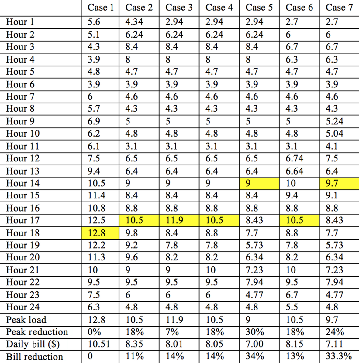
Different cases of user-defined shiftable load time interval and adjustable reduction criteria are compared in Fig. 16.

Case 1 is the most optimal schedule. Using HEMS and considering just shiftable load and no PHEV battery brings an 18% reduction in peak load. In Case 3, a PHEV battery considered as storage in the system causes the peak load to be reduced by 10%, which was associated with charging the PHEV at hour 17. By implementing the load limit in Case 4 assigned by the aggregator, this peak load is removed and the reduction is again back to 18%. By considering the load reduction criteria in Case 5 assigned by the tenant, the peak load reduction is increased by 30%. The tenant‘s level of comfort (start/end time of shiftable loads) considered in Case 6 lowers the peak load reduction to 18% compared to Case 5 and can be improved to 24% by changing the start/end time of the shiftable loads, as shown in Case 7.

As shown in Figs. 16 and 17, considering just shiftable load and no PHEV battery available (Case 2), the HEMS system brings just 11% savings in the energy bill and 18% in peak load reduction. In Case 3, the HEMS generates 14% electricity bill and 11% peak load reduction due to the extra power drawn by the PHEV at hour 17 to charge the battery. In Case 4, the aggregator assigns the load limit, which causes the PHEV not to charge its battery to maximum at hour 17; therefore, the peak load is kept lower than Case 3 and equal to Case 2 (load limit equal to Case 2 peak load).

3.1 Communication protocol

As shown in Figs. 18 and 19, CHEMS mesh networks can be established in both neighborhoods and tall buildings. In both arrangements, each unit (house, apartment) is introduced to the master HEMS as a slave HEMS node. In neighborhood CHEMS, because clear space is available, most of the nodes are connected to the network using XBee. However, in high rises, due to a lack of clear space between floors, ethernet-based communication may be used to integrate all the mesh networks deployed on each building floor.

3.2 System hardware/software control configuration

As shown in Fig. 20, CHEMS includes several slave HEMS that are numbers of apartments (houses) each containing different types of loads (residential loads) and storage units and also a community that has communal loads (lighting, pool pump) and a shared storage unit.

3.3 Scheduling methodology

Our CHEMS model is considered as an energy hub, which is a centrally integrated energy management system that serves as the core of the activity with various local energy entities. Therefore, different energy sectors including community energy resources, conversion systems, and community/mobile (PHEV) as well as community and residential loads and shared storage units are considered in this chapter.

The optimal load scheduling problem is mathematically introduced as an MILP problem. The minimization of the net load seen by the aggregator including various types of loads such as fixed, shiftable, curtailable, and storage units (community storage unit, mobile units such as PHEV and residential units) that can represent positive loads at the time of charging and negative loads at the time discharging is implemented. Different types of loads modeled in this study are:

1. (1) Fixed load: those critical loads that cannot be curtailed and shifted such as TVs, computers, electrical ranges, microwaves, and emergency lighting.
2. (2) Shiftable load: those types of noncritical loads whose operation can be deferred to the time the price of electricity is relatively lower. Resident's level of comfort and load quality of service need to be considered. Washer and dryers, pool pumps, and dishwashers are examples of this type of load.
3. (3) Adjustable load: those loads that can be curtailed seeing the hourly price of electricity or an external load reduction signal. Lighting and air conditioning systems are good examples of this type of load.
4. (4) Storage units: this type of load can be modeled as a load when they are getting charged or as generation units when they are in discharging mode. Residential storage units and PHEVs can be considered as storage units.
5. (5) Community loads: include all the loads that are common between all.

3.4 Case studies and results

Two methods of DR include: (1) price-based and (2) incentive-based DR programs (limited aggregated load), and optimal load scheduling of the building in islanded mode (microgrid) are considered in this section. Also, the proposed model is tested using the real data obtained from the Smart Home system prototype located at the Illinois Institute of Technology (IIT), DERs including 200 kW solar generation, generating in hours 11–19, and 150 kW wind generation available during hours 1–5 and 23–24, and storage units are considered in this chapter. These data are extrapolated considering the real power output generated by the wind turbine and solar panels installed at IIT.

First, optimal load scheduling is implemented in the community through price-based DR (total E(t) ≤ ∞), where E(t) represents the aggregated load. Based on a tenant's daily schedules and an appliance's quality of service, a 24-h optimal schedule is generated. Then, optimal load scheduling is implemented through incentive-based load scheduling (E(t) ≤ K). In this case, an aggregator request is delivered and, based on the amount of load curtailment submitted in the agreement, the community must curtail its load to meet that amount. Finally, the microgrid configuration of the community which is the operation of the community in islanded mode through leveraging the local generation and battery storage units to respond the building loads (E(t)=0) is studied. By using the data acquired from the Smart Home model, considering a community including 200 of these units, and applying our CHEMS model, the optimal load scheduling in the cases below is obtained.

1. (1) Case 1: community with fixed rate tariff (FRT) without PHEV and residential battery unit.
2. (2) Case 2: community price-based DR without shared PHEV and residential battery unit.
3. (3) Case 3: community price-based DR with shared PHEV and residential battery unit.
4. (4) Case 4: incentive-based DR in community using CHEMS.
5. (5) Case 5: community microgrid optimal load scheduling.

As seen in Figs. 21 and 22, Case 1 is the most nonoptimal scheduling. Because the price is fixed and load shaving and curtailing do not affect their electricity bill, there is not any encouragement for tenants to follow the price signal and change their schedule accordingly.

In Cases 2 and 3, shiftable loads are deferred to the hours with the lower hourly electricity rate (hours 1–6) and curtailable loads are adjusted to their minimum power consumption during the hours the price is higher than the tenant's setpoint. However, storage units use the available additional capacity provided by the reduced loads to charge and discharge. Consequently, although we lower the peak load by deferring the shiftable load and curtailing the adjustable load, the peak load is not decreased noticeably compared to Case 1 (about 3%). Peak load happens at hour 14 when the community storage is being charged at its maximum load to recharge the power already discharged at hour 13. So even a small oscillation in electricity price causes the storage units to charge/discharge in consecutive hours that lowers the battery lifetime as well as generates unwanted peak load. This event needs to be prevented either by considering a minimum off/on time charging/discharging consecutive cycle or assigning load limits to each community.

In Case 4, the aggregator set a load limit of 1.7 MW. This limit increases the cost by 1% compared to Cases 2 and 3. This increase happens due to the absence of demand charges imposed on residential loads. Therefore, the benefits of storage would not be noticeable compared to commercial and industrial buildings that pay the demand charge. As shown in Fig. 21, the storage unit's optimal load schedule in Case 4 was changed compared to Cases 2 and 3. Load limit schedules the storage units’ charging/discharging, and consequently prevents the community from exceeding that load limit. In this case, the charging/discharging availability of different types of storage units including community, residential, and PHEV needs to be prioritized through the introduction of different $/kW rates. Therefore, each storage unit will be charged/discharged with different rates considering the load limit set by the aggregator.

Finally, in Case 5, the model was evaluated considering the unavailability of power. As seen in Fig. 21, CHEMs will modify the loads considering the availability of DERs (residents and community) to keep the critical loads (fixed) on.