
In the last chapter we did some amazing things with one neuron, but that is hardly flexible enough to tackle more complex cases. The real power of neural networks comes into light when several (thousands, even millions) neurons interact with each other to solve a specific problem. The network architecture (how neurons are connected to each other, how they behave, and so on) plays a crucial role in how efficient the learning of a network is, how good its predictions are, and what kind of problems it can solve. There are many kinds of architectures that have been extensively studied and that are very complex, but from a learning perspective, it is important to start from the simplest kind of neural network with multiple neurons. It makes sense to start with a feed-forward neural network, where data enters at the input layer and passes through the network, layer by layer, until it arrives at the output layer (this gives the networks their name: feed-forward neural networks).
This chapter discusses networks where each neuron in a layer gets its input from all neurons from the preceding layer and feeds its output into each neuron of the next layer. As it is easy to imagine, with more complexity come more challenges. It is more difficult to get quick learning and good accuracy, since the number of hyper-parameters that are available grows due to the increase in network complexity. A simple gradient descent algorithm is not as efficient when dealing with big datasets. When developing models with many neurons, we need to have at our disposal an expanded set of tools that allow us to deal with all the challenges that those networks present.
This chapter starts looking at some more advanced methods and algorithms that will allow you to work efficiently with big datasets and big networks. These complex networks can do some interesting multiclass classifications, one of the tasks that big networks are most often required to do (for example, handwriting recognition, face recognition, image recognition, and so on), so we will use a dataset that will allow us to perform multiclass classification and study its difficulties.
We start the chapter with the network architecture and the needed matrix formalism. Next is a short overview of the new hyper-parameters that come with this new type of networks. You learn how to do multiclass classifications using the softmax function and what kind of output layer is needed. Then, before starting with the Python code, we will go into a brief digression to explain what exactly overfitting is with a simple example, and how to do a basic error analysis with complex networks.
Then we will start using Keras to construct bigger networks, applying them to a MNIST-similar dataset based on images of clothing items (the Fashion-MNIST dataset, from Zalando). Then we will look at how to add many layers in an efficient way and how to initialize the weights and the biases in the best way possible to make training fast and stable. We will look at Xavier and He initialization for the sigmoid and ReLU activation functions, respectively. Finally, we describe a rule of thumb for comparing the complexity of networks going beyond only the number of neurons. This chapter concludes with some tips on how to choose the right networks and a method to estimate the memory footprint depending on the architecture.
A Short Review of Network’s Architecture and Matrix Notation
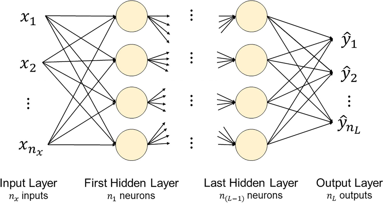
The schematic representation of a deep feed-forward neural network with many hidden layers, where each neuron gets input from each neuron in the preceding layer and feeds its output to every neuron in the next layer
L is the number of hidden layers, excluding the input layer but including the output layer
nl is the number of neurons in layer l

![$$ {w}_{ij}^{left[l
ight]} $$](https://imgdetail.ebookreading.net/2023/10/9781484280201/9781484280201__9781484280201__files__images__463356_2_En_3_Chapter__463356_2_En_3_Chapter_TeX_IEq1.png) . Figure 3-2 shows only the first two layers (input and layer 1) of the generic network from Figure 3-1, with the weights between the first neuron in the input layer and all the others in layer 1. All other neurons are grayed out for clarity.
. Figure 3-2 shows only the first two layers (input and layer 1) of the generic network from Figure 3-1, with the weights between the first neuron in the input layer and all the others in layer 1. All other neurons are grayed out for clarity.
The first two layers of a generic neural network, with the weights of the connections between the first neuron in the input layers and the others in the second layer. All other neurons and connections are drawn in light gray to make the diagram clearer

That means that the matrix W[1] has dimensions n1 × nx. This of course can be generalized between any two layers l and l − 1. Meaning that the weight matrix between two adjacent layers l and l − 1, which we indicate with W[l], will have dimensions nl × nl − 1. By convention, n0 = nx is the number of input features (not the number of observations, which we indicate with m).
The weight matrix between two adjacent layers l and l − 1, which we indicate with W[l], will have dimensions nl × nl − 1, where, by convention, n0 = nx is the number of input features.
The bias (indicated with b) will be a matrix this time. Remember that each neuron that receives inputs will have its own bias, so when considering our two layers l and l − 1 we will need nl different values of b. We indicate this matrix with b[l] and it will have dimensions nl × 1.
The bias matrix for two adjacent layers l and l − 1, which we indicate with b[l], will have dimensions nl × 1.
Output of Neurons
![$$ {hat{y}}_i^{left[1
ight]} $$](https://imgdetail.ebookreading.net/2023/10/9781484280201/9781484280201__9781484280201__files__images__463356_2_En_3_Chapter__463356_2_En_3_Chapter_TeX_IEq2.png) and let’s assume that all neurons in layer l use the same activation function that we indicate with g[l]. Then we will have
and let’s assume that all neurons in layer l use the same activation function that we indicate with g[l]. Then we will have![$$ {hat{y}}_i^{left[1
ight]}={g}^{left[1
ight]}left({z}_i^{left[1
ight]}
ight)={g}^{left[i
ight]}kern0.75em left(sum limits_{j=1}^{n_x}left({w}_{ij}^{left[1
ight]} {x}_{i,j}+{b}_i^{left[1
ight]}
ight)
ight) $$](https://imgdetail.ebookreading.net/2023/10/9781484280201/9781484280201__9781484280201__files__images__463356_2_En_3_Chapter__463356_2_En_3_Chapter_TeX_Equc.png)
![$$ {z}_i^{left[1
ight]}=sum limits_{j=1}^{n_x}left({w}_{ij}^{left[1
ight]} {x}_{i,j}+{b}_i^{left[1
ight]}
ight) $$](https://imgdetail.ebookreading.net/2023/10/9781484280201/9781484280201__9781484280201__files__images__463356_2_En_3_Chapter__463356_2_En_3_Chapter_TeX_Equd.png)
![$$ {Z}^{left[1
ight]}={W}^{left[1
ight]}X+{b}^{left[1
ight]} $$](https://imgdetail.ebookreading.net/2023/10/9781484280201/9781484280201__9781484280201__files__images__463356_2_En_3_Chapter__463356_2_En_3_Chapter_TeX_Eque.png)
Where Z[1] will have dimensions n1 × 1, and where with X we have indicated our matrix with all our observations (rows for the features and columns for observations). We assume that all neurons in layer l will use the same activation function, which we will indicate with g[l].
![$$ {Z}^{left[l
ight]}={W}^{left[l
ight]}{Z}^{left[l-1
ight]}+{b}^{left[l
ight]} $$](https://imgdetail.ebookreading.net/2023/10/9781484280201/9781484280201__9781484280201__files__images__463356_2_En_3_Chapter__463356_2_En_3_Chapter_TeX_Equf.png)
![$$ {Y}^{left[l
ight]}={g}^{left[l
ight]}left({Z}^{left[l
ight]}
ight) $$](https://imgdetail.ebookreading.net/2023/10/9781484280201/9781484280201__9781484280201__files__images__463356_2_En_3_Chapter__463356_2_En_3_Chapter_TeX_Equg.png)
where the activation function acts, as usual, element by element.
A Short Summary of Matrix Dimensions
W[l] has dimensions nl × nl − 1 (where we have n0 = nx by definition)
b[l] has dimensions nl × 1
Z[l − 1] has dimensions nl − 1 × 1
Z[l] has dimensions nl × 1
Y[l] has dimensions nl × 1
In each case, l goes from 1 to L.
Example: Equations for a Network with Three Layers

A practical example of a feed-forward neural network
![$$ {hat{Y}}^{left[1
ight]}={g}^{left[1
ight]}left({W}^{left[1
ight]}X+{b}^{left[1
ight]}
ight), $$](https://imgdetail.ebookreading.net/2023/10/9781484280201/9781484280201__9781484280201__files__images__463356_2_En_3_Chapter__463356_2_En_3_Chapter_TeX_IEq3.png) whereby W[1] has dimensions 3 × nx, b has dimensions 3 × 1, and X has dimensions nx × m
whereby W[1] has dimensions 3 × nx, b has dimensions 3 × 1, and X has dimensions nx × m![$$ {hat{Y}}^{left[2
ight]}={g}^{left[2
ight]}left({W}^{left[2
ight]}{hat{Y}}^{left[1
ight]}+{b}^{left[2
ight]}
ight), $$](https://imgdetail.ebookreading.net/2023/10/9781484280201/9781484280201__9781484280201__files__images__463356_2_En_3_Chapter__463356_2_En_3_Chapter_TeX_IEq4.png) whereby W[2] has dimensions 2 × 3, b has dimensions 2 × 1, and
whereby W[2] has dimensions 2 × 3, b has dimensions 2 × 1, and ![$$ {hat{Y}}^{left[1
ight]} $$](https://imgdetail.ebookreading.net/2023/10/9781484280201/9781484280201__9781484280201__files__images__463356_2_En_3_Chapter__463356_2_En_3_Chapter_TeX_IEq5.png) has dimensions 3 × m
has dimensions 3 × m![$$ {hat{Y}}^{left[3
ight]}={g}^{left[3
ight]}left({W}^{left[3
ight]}{hat{Y}}^{left[2
ight]}+{b}^{left[3
ight]}
ight), $$](https://imgdetail.ebookreading.net/2023/10/9781484280201/9781484280201__9781484280201__files__images__463356_2_En_3_Chapter__463356_2_En_3_Chapter_TeX_IEq6.png) whereby W[3] has dimensions 1 × 2, b has dimensions 1 × 1, and
whereby W[3] has dimensions 1 × 2, b has dimensions 1 × 1, and ![$$ {hat{Y}}^{left[2
ight]} $$](https://imgdetail.ebookreading.net/2023/10/9781484280201/9781484280201__9781484280201__files__images__463356_2_En_3_Chapter__463356_2_En_3_Chapter_TeX_IEq7.png) has dimensions 2 × m
has dimensions 2 × m
The network output ![$$ {hat{Y}}^{left[3
ight]} $$](https://imgdetail.ebookreading.net/2023/10/9781484280201/9781484280201__9781484280201__files__images__463356_2_En_3_Chapter__463356_2_En_3_Chapter_TeX_IEq8.png) will have, as expected, dimensions 1 × m.
will have, as expected, dimensions 1 × m.
All this may seem rather abstract (and in fact it is). You will see later in the chapter how easy it is to implement in Keras simply building the right architecture, based on the steps just discussed.
Hyper-Parameters in Fully Connected Networks
In networks as the ones just discussed, there are quite a few parameters that you can tune to find the best model for your problem.
Parameters that you fix at the beginning and then do not change during the training phase are called hyper-parameters (like the number of epochs).
The number of layers, L
The number of neurons in each layer ni for i, from 1 to L
The choice of activation function for each layer g[l]
The number of iterations (or epochs)
The learning rate
A Short Review of the Softmax Activation Function for Multiclass Classifications
You still need to suffer a bit more theory before getting to some TensorFlow code. These kinds of networks start to be complex enough to be able to perform multiclass classifications with reasonable results. To do this, we must introduce the softmax function.


So S(z)i behaves like a probability since its sum over i is 1 and its elements are all less than 1. We will look at S(z)i as a probability distribution over k possible outcomes. For this example, S(z)i will simply be the probability of our input observation of being of class i. Let’s suppose we are trying to classify an observation into three classes. We may get the following output: S(z)1 = 0.1, S(z)2 = 0.6, and S(z)3 = 0.3. That means that the observation has a 10% probability of being in class 1, a 60% probability of being in class 2, and a 30% probability of being in class 3. Normally, you would choose to classify the input observation into the class with the higher probability—in this example, class 2 with 60% probability.
We will look at S(z)i with i = 1, …, k as a probability distribution over k possible outcomes. For this example, S(z)i will simply be the probability of our input observation being in class i.
To be able to use the softmax function for classification, we need to use a specific output layer. We need to use ten neurons (in the case of a ten-class multiclass classification problem, like the one we see later in the chapter), where each will give zi as its output and then one neuron that will output S(z). This neuron will have the softmax function as the activation function and will have as inputs the ten outputs zi of the last layer with ten neurons. In Keras, you use the tf.keras.activations.softmax function applied to the last layer with ten neurons. Remember that this Keras function will act element by element. You will a concrete example from start to finish on how to implement this practically later in this chapter.
A Brief Digression: Overfitting
One of the most common problems that you will encounter when training deep neural networks is overfitting. Your network may, due to its flexibility, learn patterns that are due to noise, errors, or simply wrong data. It is very important to understand what overfitting is, so now we will go through a practical example of what can happen, to get an decent understanding of it. To make it easier to visualize, we will work with a simple two-dimensional dataset created for this purpose.
A Practical Example of Overfitting


To add some random noise to the function, we used the np.random.normal(0, 1, size = len(x)) function, which generates a NumPy array of random values from a normal distribution of length len(x) with average 0 and standard deviation 1.

The data we generated with a = 1, b = 2, and c = 3

The linear model misses the main feature of the data being too simple. In this case, the model has high bias
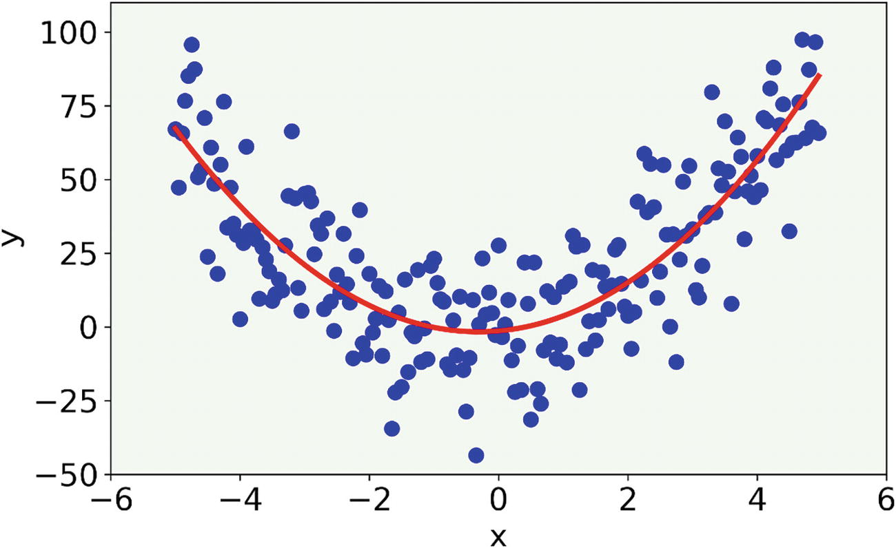
The result (red line) for a two-degree polynomial

The results for a 21-degree polynomial model
This model shows features that we know are wrong (since we created our data). Those features are not present, but the model is so flexible that it captures the random variability that we introduced with noise. The oscillations that have appeared using this high-ordered polynomial are wrong and do not describe the data correctly.
In this case, we talk about overfitting, meaning we start capturing with our model features that are due to random error, for example. It is easy to understand that this generalizes quite badly. If we applied this 21-degree polynomial model to new data it would not work well, since the random noise would be different in the new data and so the oscillations (the ones represented in Figure 3-7) would make no sense.
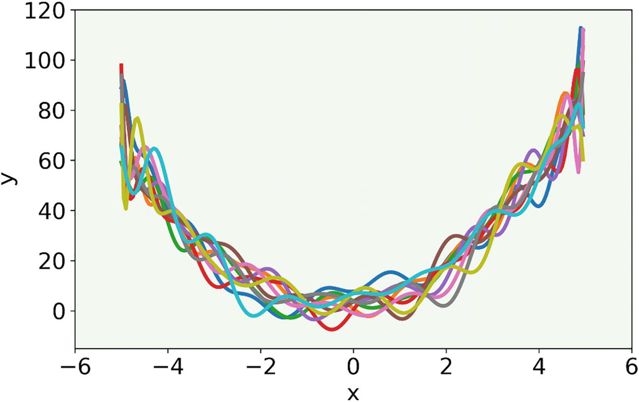
The result of our model with a 21-degree polynomial fitted to ten different datasets generated with different random noise values

The result of the linear model applied to data where we have randomly changed the random noise. For easier comparison with Figure 3-8, we used the same scale
You can see that the model is much more stable. The linear model does not capture features that are dependent from the noise, but it misses the main features of the data (the concave nature). We talk here of high bias.
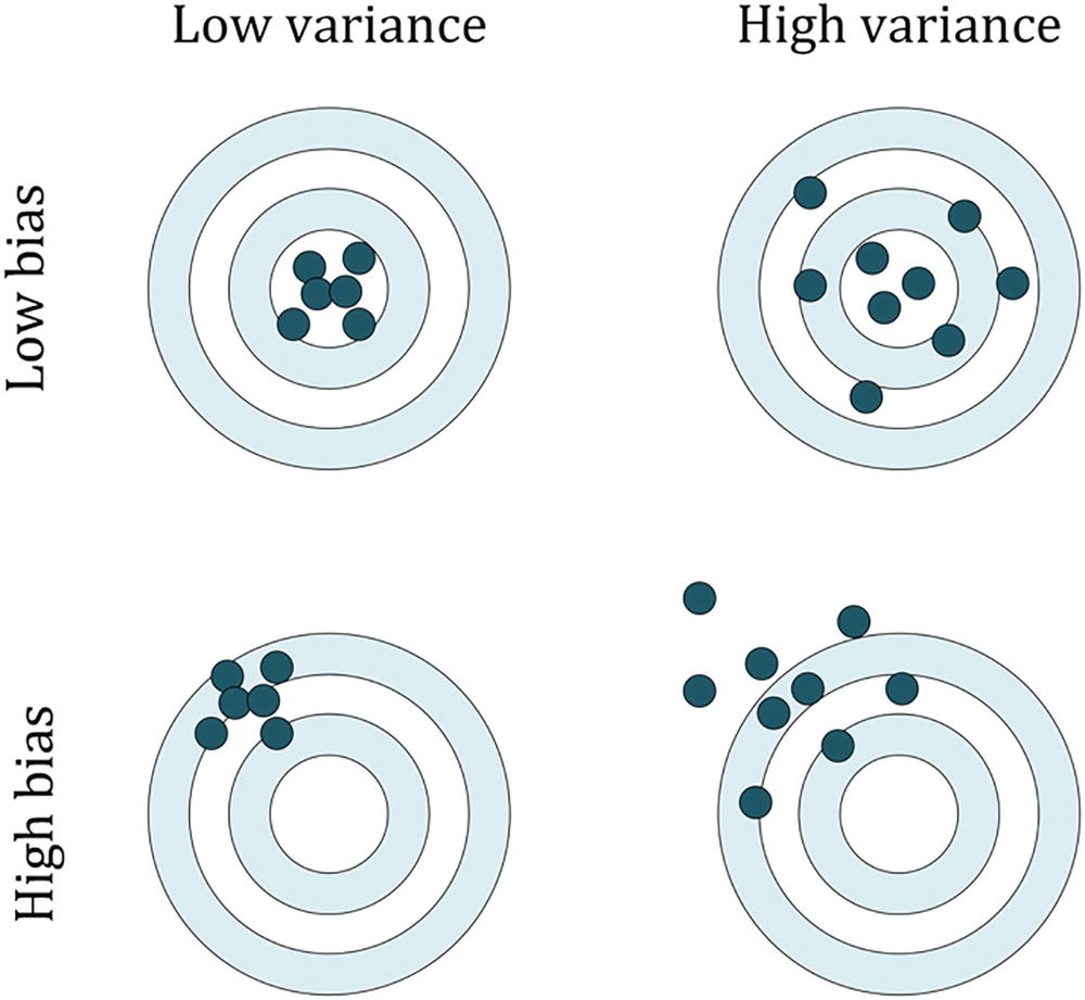
Bias is a measure of how close the measurements are to the true values (the center in the figure) and variance is a measure of how spread the measurements are around the average (not necessarily the true value, as you can see on the left)
In the case of neural networks, we have many hyper-parameters (number of layers, number of neurons in each layer, activation function, and so on) and it is very difficult to know in which regime we are. How can we tell if our model has a high variance or a high bias, for example? An entire chapter is dedicated to this subject, but the first step to performing this error analysis is to split the dataset in two different subsets. Let’s see what that means and why we have to do it.
The essence of overfitting is to have unknowingly extracted some of the residual variation (i.e., the noise) as if that variation represented underlying model structure [1]. The opposite is called underfitting, when the model cannot capture the structure of the data.
The problem with overfitting and deep neural networks is that there is no way of easily visualizing the results. Therefore we need a different approach to determine if our model is overfitting, underfitting, or is just right. This can be achieved by splitting the dataset into different parts and comparing the metrics of the parts. You learn about the basic idea in the next section.
Basic Error Analysis
Training dataset: The model is trained on this dataset using the inputs and the relative labels and using an optimizer algorithm like gradient descent. Often this is called the training set.
Development (or validation) set: The trained model will then be used on this dataset to check how it is doing. On this dataset we will test different hyper-parameters. For example, we can train two different models with a different number of layers on the training dataset and test them on this dataset to check how they are doing. Often this is called the dev set.
Examples of the Difference Between Models with High Bias and Models with High Variance
Error | Case A | Case B | Case C | Case D |
|---|---|---|---|---|
Train set error | 1% | 15% | 14% | 0.3% |
Dev set error | 11% | 16% | 32% | 1.1% |
Case A: We are overfitting (high variance), because we are doing very well on the training set, but our model generalizes very badly to our dev set (see Figure 3-8 again).
Case B: We see a problem with high bias, meaning that our model is not doing very well generally, on both datasets (see Figure 3-9 again).
Case C: We have a high bias (the model cannot predict the training set very well) and high variance (the model does not generalize on the dev set very well).
Case D: Everything seems okay. There is good error on the training set and good data on the dev set. It is a good candidate for our best model.
We will explain much better all those concepts later in the book, where we provide recipes on how to solve problems of high bias, high variances, both, and even more complex cases.
To recap, to do a very basic error analysis, you need to split your dataset into at least two sets: train and dev. You should then calculate your metric on both sets and compare them. You want to have a model that has low error on the train set, low error on the dev set (as with Case D in the previous example), and the two values should be comparable.
Your main take away from this section should be two-fold: 1) you need a set of recipes and guidelines for understanding how your model is doing: is it overfitting, underfitting, or is it just right? 2) to answer question 1 and perform the analysis, you need to split the dataset into two parts (later in the book, you will also see what you can do with the dataset split in three or even four parts).
Implementing a Feed-Forward Neural Network in Keras
As you can see, we added more neurons (15) to the hidden layer (that in the one-neuron model was already the output one) and we added the output layer, made of ten neurons, since we have ten classes. As you can notice, you can easily create very complex models by simply adding to the stack one layer after another.
In the next paragraphs, you will see a practical example about how you use this model, choosing the right activation function and the right loss function (given as additional parameters) to solve a multiclass classification task.
Multiclass Classification with Feed-Forward Neural Networks
The task we are going to solve together is a multiclass classification problem on the Zalando dataset. It consists of predicting the corresponding label among ten possible cases (ten different types of clothing). To solve it, we will use a feed-forward network architecture and try different configurations (different optimizers and architectures), performing some error analysis to see which situation is better. Let’s start by looking at the data.
The Zalando Dataset for the Real-World Example
Zalando SE is a German commerce company based in Berlin . The company maintains a cross-platform store that sells shoes, clothing, and other fashion items [2]. For a Kaggle competition, they prepared a MNIST-similar dataset of Zalando’s clothing article images [4], where they provided 60000 training images and 10000 test images. (If you do not know what Kaggle is, check out their website [3], where you can participate in many competitions where the goal is to solve problems with data science.) As in MNIST, each image is 28x28 pixels in grayscale. They classified all images in ten different classes and provided the labels for each image. The dataset has 785 columns, where the first column is the class label (an integer going from 0 to 9) and the remaining 784 contain the pixel gray value of the image (you can calculate that 28x28=784).
0: T-shirt/top
1: Trouser
2: Pullover
3: Dress
4: Coat
5: Sandal
6: Shirt
7: Sneaker
8: Bag
9: Ankle boot

One example from each of the ten classes in the Zalando dataset
The dataset has been provided under the MIT License4. The datafile can be downloaded from Kaggle (https://www.kaggle.com/zalando-research/fashionmnist/data) or directly from GitHub (https://github.com/zalandoresearch/fashion-mnist). If you choose the second option, you need to prepare the data a bit (you can convert it to CSV with the script located at https://pjreddie.com/projects/mnist-in-csv/). If you download it from Kaggle, you have all the data in the right format. You will find two CSV files zipped on the Kaggle website. The ZIP file contains fashion-mnist_train.csv, with 60000 images (roughly 130 MB) and fashion-mnist_test.csv, with 10000 (roughly 21 MB).
In our example, we will retrieve the dataset in a third way: from the TensorFlow datasets catalog (https://www.tensorflow.org/datasets/catalog/fashion_mnist), since in this way we will not have to perform any preprocessing steps and we will automatically import the data inside our notebook. Now, let’s code!
Incredibly easy! Now we have two numpy matrices (trainX and testX) containing all the pixel values describing each of the training and test images and two NumPy arrays (trainY and testY) containing the associated labels.
Remember that you should not focus on the Python implementation. Focus on the model, on the concepts behind the implementation. You can achieve the same results using pandas, NumPy, or even C. Try to concentrate on how to prepare the data, how to normalize it, how to check the training, and so on.
As you can see, we have a training dataset made of 60000 items, stored as images of 28x28 pixels each, and a test dataset made of 10000 items, stored in the same way. Then, an array of corresponding labels is associated with each dataset.
Now we need to modify our data to obtain a “flattened” version of image, meaning an array of 754 pixels, instead of a matrix of 28x28 pixels. This step is necessary, because, as we saw when we discussed the feed-forward network architecture, it receives as inputs all the features as separate values. Therefore, we need to have all the pixels stored in the same array. On the contrary, Convolutional Neural Networks (CNNs) do not work with flattened versions of the images, but that’s a topic for Chapter 7. For now, keep this in mind.
labels: Has dimensions (60000) and contains the class labels (integers from 0 to 9)
train: Has dimensions m × nx (60000x784) and contains the features, where each column contains the grayscale value of a single pixel in the image (remember 28x28=784)
Before developing the network, we need to solve another problem. Labels must be provided in a different form when performing a multiclass classification task.
Modifying Labels for the Softmax Function: One-Hot Encoding

where yi contains our labels and  is the result of our network. So, the two elements must have the same dimensions. In our case we saw that our network will give as output a vector with ten elements, while a label in our dataset is simply a scalar. So, we have
  that has dimensions (10,1) and yi that has dimensions (1,1). This will not work if we do not do something smart. We need to transform our labels in a vector that have dimensions (10,1). A vector with a value for each class, but what value should we use?
Examples of How One-Hot Encoding Works. Remember that Labels Go from 0 to 9, as Indexes
Label | One-Hot Encoded Label |
|---|---|
0 | (1,0,0,0,0,0,0,0,0,0) |
2 | (0,0,1,0,0,0,0,0,0,0) |
5 | (0,0,0,0,0,1,0,0,0,0) |
7 | (0,0,0,0,0,0,0,1,0,0) |
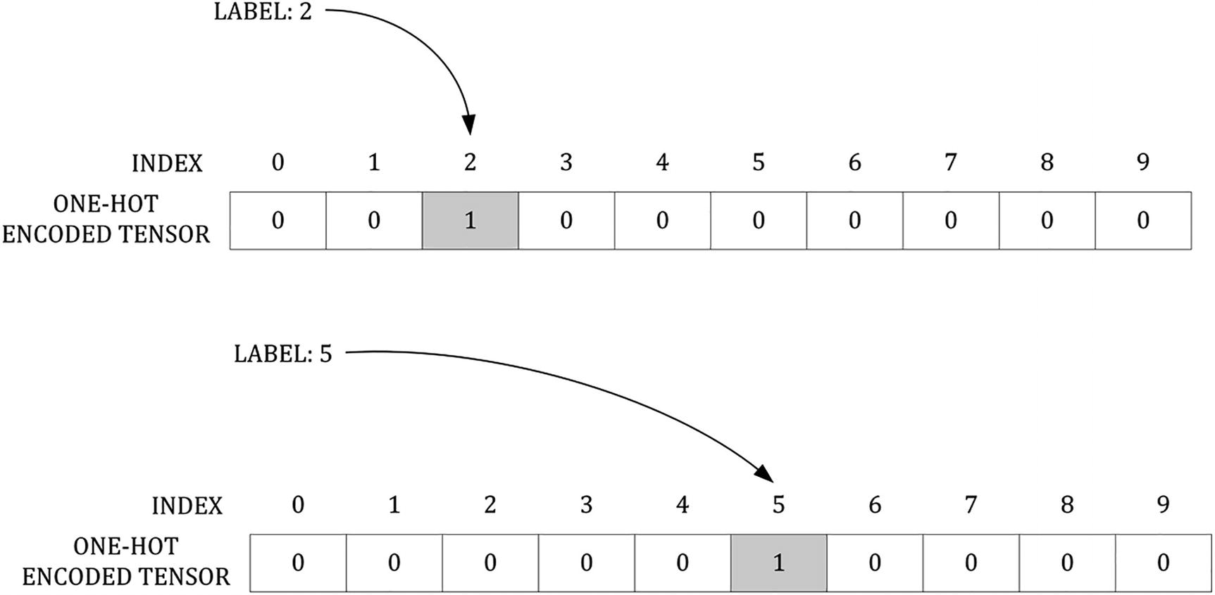
A graphical representation of the process of one-hot encoding a label. Two labels (2 and 5) are one-hot encoded in two vectors. The grayed element of the vector is the one the becomes 1, while the white marked ones remain 0
First you create a new array with the right dimensions: (60000,10), and then you fill it with zeros with the NumPy function np.zeros((60000,10)). Then you set to 1 only the columns related to the label itself, using pandas functionalities to slice dataframes with the line labels_train[np.arange(60000), trainY] = 1 (the same of course is also performed in the case of the test dataset). In the end, you obtain the dimensions (60000,10), where each row indicates a different observation.
Now we can compare yi and  since both have the dimensions (10,1) for one observation, or when considering the entire test dataset of (10000,10). The same can of course be asserted for the training dataset. Each column in
  will represent the probability of our observation being of a specific class. At the very end when calculating the accuracy of our model, we will assign the class with the highest probability to each observation.
Our network will give us the ten probabilities for the observation of being of each of the ten classes. At the end, we will assign to the observation the class that has the highest probability.
The Feed-Forward Network Model

The network architecture with a single hidden layer. We will vary the number of neurons n1 in the hidden layer during our analysis


We create an output layer with ten neurons, in this way we will have our ten values as output.
Then we feed the ten values into a new neuron (let’s call it “softmax” neuron) that will take the ten inputs and give as output ten values that are all less than one, which adds to 1.

In Keras, this is straightforward. But it is instructive to know exactly what each line of code does. That is what the Keras function model.add(Dense(10, activation = 'softmax')) does. It takes a vector as the input and returns a vector with the same dimensions as the input, but “normalized,” as discussed above. In other words, if we feed z = (z1 z2 … z10) into the function, it will return a vector with the same dimensions as z, meaning 1x10, where each element added to the others gives 1.
Keras Implementation
Our last layer will use the softmax function: model.add(Dense(10, activation = 'softmax')).
The two parameters—15 (n1) and 10 (n2)—define the number of neurons in the different layers. Remember the second (output) layer must have ten neurons to be able to use the softmax function. But we will play with the value of n1. Increasing n1 will increase the complexity of the network.
We set the categorical cross-entropy (loss = 'categorical_crossentropy') as the loss function and the categorical accuracy (metrics = ['categorical_accuracy']) as the metrics. The reason for this choice is that we have hot-encoded the labels and therefore the categorical versions of these functions are needed.
We have set as the optimizer the standard version of the gradient descent . The biggest problem is that the model, as we coded it, will create a huge matrix for all observations (that are 60,000) and then will modify the weights and bias only after a complete sweep over all observations. This requires a lot of resources, memory, and CPU. If that was the only choice we have, we would have been doomed. Keep in mind that in the deep learning world, 60,000 examples of 784 features is not a big dataset at all. We need to find a way of letting this model learn faster.
Moreover, notice that, when training the model, we have set batch_size = data_train_norm.shape[0] inside the Keras fit method. Keras by default sets the batch size to 32 observations [5], but the batch gradient descent updates weights and biases after all training observations have been seen by the network. Therefore, we need to change this parameter to obtain the basic version of gradient descent.
In the same way, we need to set the momentum = 0.0 inside the method tf.keras.optimizers.SGD. To summarize, since Keras does not include a function to perform the standard gradient descent, we used the stochastic gradient descent function, setting the momentum to zero and the batch size to the entire number of observations.
To do some basic error analysis, you also need the dev dataset, which we loaded and prepared in the previous paragraphs.
Do not get confused by the fact that the filename contains the word test. Sometimes the dev dataset is called the test dataset. When we discuss error analysis later in the book, we use three datasets: train, dev, and test. To remain consistent in the book, we use the name dev here as well, not to confuse you with different names in different chapters.
To recap, we applied the model trained on the 60,000 observations to the dev test (made up of 10,000 observations) and then calculated the accuracy on both datasets.
A good exercise is to include this calculation in your model so that your build_model() function automatically returns the two values.
Gradient Descent Variations Performances
In Chapter 2, we looked at the different GD variations and discussed their advantages and disadvantages. Let’s know see how they differ in a practical case.
Comparing the Variations
Comparing the Performances of Three Variations of Gradient Descent
Gradient Descent Variation | Running Time | Final Value of Cost Function | Accuracy |
|---|---|---|---|
Batch gradient descent | 0.35 min | 1.86 | 43% |
Stochastic gradient descent | 60.23 min | 0.26 | 91% |
Mini-batch gradient descent (mini-batch size = 50) | 1.70 min | 0.26 | 90% |
Now you can see that mini-batch gradient descent is definitely the best compromise in terms of execution time and classification performance. Now you should be convinced that it is currently the preferred method to be used as an optimizer in deep neural networks, among the different gradient descent types, since it can reach high performance, maintaining a good trade-off between performance and execution time.

A comparison of speed of convergence of the mini-batch gradient descent algorithm with different mini-batch sizes. The learning rate used for this figure was γ = 0.0001. Note that the time needed by each case is not the same. The smaller the mini-batch size, the more time the algorithm needs
The best compromise between running time and convergence speed (with respect to the number of epochs) is achieved using the mini-batch gradient descent. The optimal size of the mini-batches is dependent on your problem, but small numbers like 30 or 50 are a good place to start. You will find a compromise between running time and convergence speed.
To get an idea of how the running time depends on what value the cost function can reach after 100 epochs, see Figure 3-15 (in comparison to Chapter 2, the times are evaluated with a real dataset). Each point is labeled with the size of the mini-batch used in that run. You can see that decreasing the mini-batch size decreases the value of J after 100 epochs. This happens quickly, without increasing the running time significantly, until you arrive at a value for the mini-batch size that is around 20. At that point, the time starts to increase quickly and the value of J after 100 epochs does not decrease and flattens out.
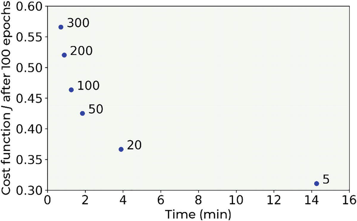
The plot shows the value of the cost function after 100 epochs for the Zalando dataset vs. the running time needed to run through 100 epochs. Note that the points are single runs, and the plot is only indicative of the dependency. Running time and cost function have a small variance when evaluated over several runs. This variance is not shown in the plot
Writing a function with the hyper-parameters as inputs is common practice. This allows you to test different models with different values for the hyper-parameters and check which ones are better.
Examples of Wrong Predictions

One example of incorrectly classified images for each class. Over each image, the True class (labeled with “True”) and the predicted (labeled with “Pred”) class are reported. This model has one hidden layer with 15 neurons, has been run for 1000 epochs with a learning rate of 0.0001
Some errors are understandable, such as where a coat was wrongly classified as a pullover. We could easily make the same mistake. The wrongly classified dress is, on the other hand, easy for a human to get right.
Weight Initialization
If you tried to run the code, you will have realized that the convergence of the algorithm is strongly variable, and it depends on the way you initialize your weights. In the previous sections, we focused on understanding how such a network works to not get distracted by additional information, but it is time to look at this problem a bit more closely, since it plays a fundamental role in many layers.
![$$ {z}_i=sum limits_{j=1}^{n_x}left({w}_{ij}^{left[1
ight]} {x}_{i,j}+{b}_i^{left[1
ight]}
ight) $$](https://imgdetail.ebookreading.net/2023/10/9781484280201/9781484280201__9781484280201__files__images__463356_2_En_3_Chapter__463356_2_En_3_Chapter_TeX_Equr.png)
Normally, in a deep network, the number of weights is quite big, so you can easily imagine that if the ![$$ {w}_{ij}^{left[1
ight]} $$](https://imgdetail.ebookreading.net/2023/10/9781484280201/9781484280201__9781484280201__files__images__463356_2_En_3_Chapter__463356_2_En_3_Chapter_TeX_IEq13.png) are big, the quantity zi can be quite big, and then the ReLU activation function can return a nan value since the argument is too big for Python to calculate it properly (remember that in a classification problems, you have a log() function and therefore values of the argument as zero for example are not acceptable). So, you want the zi to be small enough to avoid an explosion of the output of the neurons, and big enough to avoid having the outputs die out and making the convergence a very slow process.
are big, the quantity zi can be quite big, and then the ReLU activation function can return a nan value since the argument is too big for Python to calculate it properly (remember that in a classification problems, you have a log() function and therefore values of the argument as zero for example are not acceptable). So, you want the zi to be small enough to avoid an explosion of the output of the neurons, and big enough to avoid having the outputs die out and making the convergence a very slow process.
Some Examples of Weight Initialization for Deep Neural Networks
Activation Function | Standard Deviation σ for a Given Layer |
|---|---|
Sigmoid |
|
ReLU |
|


For Sigmoid activation function.
Using this initialization can speed up training considerably and is the standard way that many libraries initialize weights (for example, the Caffe library).
In Keras, weight initialization is straightforward by means of the tf.keras.initializers function. Look at the Keras documentation to see which initialization strategies are available [7].
Adding Many Layers Efficiently
First we define the dimensions of the input layer.
Then we define the first hidden layer (the number of neurons is given as the function’s input).
Then we add the other hidden layers one at a time. The number of layers is given as the function’s input.
We then add the output layer and we stack all the layers together inside the model.
We then compile and train the model, returning its performance.
Notice that in the previous code, we used Keras functional API (see Appendix A if you are not sure how it works), a functionality that provides a more flexible way to create models with respect to the tf.keras.Sequential API. With this functionality, we easily created a model with a customizable number of layers and neurons per layer.
The code is now much easier to understand, and you can use it to create networks as big as you want.
One layer and ten neurons each layer
Two layers and ten neurons each layer
Three layers and ten neurons each layer
Four layers and ten neurons each layer
Four layer and 100 neurons each layer

The cost function vs. epochs for five models
In case you are wondering, the model with four layers, each with 100 neurons, which seems much better than the others, is starting to go in the overfitting regime, with a train set accuracy of 91% and of 87% on the dev set (after only 200 epochs).
Advantages of Additional Hidden Layers
It is instructive to play with the models. Try varying the number of layers, the number of neurons, how you initialize the weights, and so on. If you invest some time you can reach an accuracy of over 90% in a few minutes of running time, but that requires some work. If you try several models you may realize that in this case using several layers does not seem to bring benefits versus a network with just one. This is often the case.
Theoretically speaking, a one-layer network can approximate every function you can imagine, but the number of neurons needed may be very large and therefore the model becomes less useful. Now the catch is that the ability of approximating a function does not mean that the network can do it, due for example to the sheer number of neurons involved or the time needed.
Empirically it has been shown that networks with more layers require a much smaller number of neurons to reach the same results and usually generalize better to unknown data.
Theoretically speaking, you do not need to have multiple layers in your networks, but often in practice you should. It is almost always a good idea to try a network with several layers and a few neurons in each instead of a network with one layer populated by a huge number of neurons. There is no set rule on how many neurons or layers are best. You should try starting with low numbers of layers and neurons and then increase them until your results stop getting better.
In addition, having more layers may allow your network to learn different aspects of your inputs. For example, one layer may learn to recognize vertical edges of an image, and another horizontal ones. Remember that in this chapter we discussed networks where each layer is identical (up to the number of neurons) to all the others. You will learn in Chapter 7 how to build networks whereby the layers perform very different tasks and are structured very differently from each other, making this kind of network much more powerful for certain tasks with respect to the models we discussed in this chapter.
As a simple example, imagine predicting the selling prices of houses. In this case a network with several layers may learn more information on how the features relate to the price. For example, the first layer may learn basic relationships, such as bigger houses mean higher prices. But the second layer may learn more complex features, such as a big house with a small number of bathrooms means a lower selling price.
Comparing Different Networks

The cost functionis decreasing vs. epochs for a neural network, with one hidden layer and 1, 5, 15, and 30 neurons. The calculations have been performed with mini-batch gradient descent with a batch size of 50 and a learning rate of 0.0001
![$$ {Q}^{left[l
ight]}={n}_l{n}_{l-1}+{n}_l={n}_lleft({n}_{l-1}+1
ight) $$](https://imgdetail.ebookreading.net/2023/10/9781484280201/9781484280201__9781484280201__files__images__463356_2_En_3_Chapter__463356_2_En_3_Chapter_TeX_Equy.png)

Examples of Different Network Architectures and Their Corresponding Q Parameters
Network Architecture | Parameter Q (Number of Learnable Parameters) | Number of Neurons |
|---|---|---|
Network A: 784 features, 2 layers: n1 = 15, n2 = 10 | QA = 15(784 + 1) + 10 ∗ (15 + 1) = 11935 | 25 |
Network B: 784 features, 16 layers: n1 = n2 = … = n15 = 1, n16 = 10 | QB = 1 ∗ (784 + 1) + 1 ∗ (1 + 1) + … + 10 ∗ (1 + 1) = 923 | 25 |
Network C: 784 features, 3 layers: n1 = 10, n2 = 10, n3 = 10 | QC = 10 ∗ (784 + 1) + 10 ∗ (10 + 1) + 10 ∗ (10 + 1) = 8070 | 30 |
Draw your attention to networks A and B. Both have 25 neurons, but the QA parameter is much bigger (more than a factor of ten) than QB. You can imagine how network A will be much more flexible in learning than network B, even if the number of neurons is the same.
Q in practice is not a measure of how complex or how good a network is. It may well happen that, of all the neurons, only a few will play a role, therefore calculating Q in this way does not tell the entire story. There is a vast amount of research on the so-called effective degrees of freedom of deep neural networks but that would go way beyond the scope of this book. But this parameter gives a good rule of thumb for deciding if the set of models you want to test are in a reasonable complexity progression.
Network Architectures Tested in Figure 3-18 with their Corresponding Q Parameters
Network Architecture | Parameter Q (Number of Learnable Parameters) | Number of Neurons |
|---|---|---|
784 features, 1 layer with 1 neuron, 1 layer with ten neurons | Q = 1 ∗ (784 + 1) + 10 ∗ (1 + 1) = 895 | 11 |
784 features, 1 layer with 5 neuron, 1 layer with ten neurons | Q = 5 ∗ (784 + 1) + 10 ∗ (5 + 1) = 3985 | 15 |
784 features, 1 layer with 15 neuron, 1 layer with ten neurons | Q = 15 ∗ (784 + 1) + 10 ∗ (15 + 1) = 11935 | 25 |
784 features, 1 layer with 30 neuron, 1 layer with ten neurons | Q = 30 ∗ (784 + 1) + 10 ∗ (30 + 1) = 23860 | 40 |


You should be able to solve a quadratic equation, so we will only look at the solution here. This equation is solved for a value of nB = 14.4, but since we cannot have 14.4 neurons, we will need to use the closest integer, nB = 14. For nB = 14, we will have QB = 11560, a value very close to 11935.
The fact that the two networks have the same number of learnable parameters does not mean that they can reach the same accuracy and does not even mean that if one learns very quickly the second will learn at all!
The model with three layers, each with 14 neurons, could be a good starting point for further testing.
Let’s discuss another point that is important when dealing with a complex dataset. Consider the first layer. Let’s suppose we consider the Zalando dataset and we create a network with two layers: the first with one neuron and the second with many. All the complex features that your dataset has may well be lost in your single first neuron, since it will combine all features into a single value and pass the same value to all the other neurons of the second layer.
Tips for Choosing the Right Network
You have discussed a lot of cases, you have seen a lot of formulas, but how can you decide how to design your network?
When considering a set of models (or network architectures) you want to test, a good rule of thumb is to start with a less complex one and move to more complex ones. A rule of thumb to estimate the relative complexity (to make sure that you are moving in the right direction) is the Q parameter .
If you cannot reach good accuracy if any of your layers has a particular low number of neurons. This layer may kill the effective capacity of learning from a complex dataset of your network. Consider for example the case with one neuron in Figure 3-18. The model cannot reach low values for the cost function because the network is too simple to learn from a complex dataset like the Zalando one.
Remember that a low or high number of neurons is always relative to the number of features you have. If you have only two features in your dataset, one neuron may well be enough, but if you have a few hundred (like in the Zalando dataset, where nx = 784), you should not expect one neuron to be enough.
Which architecture you need is also dependent on what you want to do. It’s always worth checking the online literature to see what others have already discovered about specific problems. For example, it’s well known that for image recognition, convolutional networks are very good, so they would be a good choice.
When moving from a model with L layers to one with L + 1 layers, it’s always a good idea to start with the new model and use a slightly smaller number of neurons in each layer and then increase it step by step. Remember that more layers have a chance of learning complex features more effectively, so if you are lucky fewer neurons may be enough. It is something worth trying. Always keep track of your optimizing metric for all your models. When you are not getting much improvement anymore, it may be worth trying completely different architectures (maybe convolutional neuronal networks, etc.).
Estimating the Memory Requirements of Models

- Parameters: In memory, you need to keep the parameters, their gradients during backpropagation, and also additional information if the optimization is using momentum, Adagrad, Adam, or RMSProp optimizers. A good rule of thumb in order to account for all these factors6 is to multiply the memory taken by the weights alone by roughly 3. With the notation we have used so far, the memory used from parameters (indicated with MW) in Gb would be

- Activations: Each neuron output must be stored, normally with their gradient for backpropagation. Conservatively only a mini-batch will need to be kept in memory. Calling SMB the mini-batch size the memory needed for activations MA in Gb can be written as

- Miscellaneous: This part includes the data that must be loaded into memory and so on. For the purposes of a rough estimate, the memory taken here MM will be estimated only with the dataset size. In the case of MNIST, that will be (in Gb) given by the following equation. Each pixel value, although originally an INT8, must be converted to floating-point 64-data type to perform the training


Note that this is just a rough indication and will not be precise since the amount of memory taken by a model may depend on software versions, the operating system, and many more factors. If we solve the last equation for n for example, we can get a very good estimate of the biggest FFNN network that could be run on such a device when applied to MNIST. For example, consider the case of a Raspberry Pi 4 with 2 GB of memory. Typically, such a system has roughly MD = 1.7 GB free at any moment. So for a network with NL = 2 and SMB = 128, the last equation will give a solution of n ≈ 8200. Indeed, trying to train a network with more than 8200 neurons on such a device will give a memory error on the device, since there is not enough memory to keep everything available in RAM. (If you test it, your results may vary, depending as mentioned on which version of the Raspberry Pi you have, which version of TensorFlow you are using, and so on.)
For practical purposes to get a rougher estimate, you can neglect the linear terms in n in the last equation and still get a usable guideline. For example, in the example discussed previously, neglecting the linear term would give an estimate of n ≈ 8700. Higher than the actual one, but one that will give useful rough information about the maximum number of usable neurons. Finally, remember that only a practical test will guarantee that a specific model can run on a low-memory device.
General Formula for the Memory Footprint


This accounts for the fact that the dataset size is not 60000 but m and that the input dimension is not 784 but nx.
Exercises
Apply He weight initialization to the multiclass classification problem you saw in this chapter to see if you can speed up the learning phase.
Try to optimize the feed-forward neural network built in this chapter to reach the best possible accuracy (without overfitting the training dataset!). Tune the number of epochs, the learning rate, the optimizer, the number of neurons, the layers, and the mini-batches. Hint: Write a function like the one we used to test different numbers of layers and neurons and give it as inputs all the tunable parameters.
Consider the regression problem we solved with a model made by a single neuron (predicting radon activity in U.S. houses). Try to build a feed-forward neural network to solve the same regression task. See if you can get better prediction performance. Hint: You will need to change the loss function and the metrics to evaluate your results, and one-hot encoding will not be necessary anymore. As a starting point, you can find the entire code in the online version of the book at https://adl.toelt.ai.
References
[1] Burnham, K. P.; Anderson, D. R. (2002), Model Selection and Multimodel Inference (2nd ed.), Springer-Verlag.
[2] https://en.wikipedia.org/wiki/Zalando, last accessed 16.02.2021.
[3] www.kaggle.com, last accessed 16.02.2021.
[4] Xiao, Han, Kashif Rasul, and Roland Vollgraf. “Fashion-mnist: a novel image dataset for benchmarking machine learning algorithms.” arXiv preprint arXiv:1708.07747 (2017).
[5] https://keras.io/api/models/model_training_apis/#fit-method, last accessed 14/03/2021.
[6] “Understanding the Difficulty of Training Deep Feedforward neural networks”, X. Glorot, Y. Bengio (2010), https://goo.gl/bHB5BM.
[7] https://www.tensorflow.org/api_docs/python/tf/keras/initializers, last accessed 23.02.2021.