
After reading about learning with neural networks in the previous chapter, you are now ready to explore their most fundamental component, the neuron. In this chapter, you learn the main components of the neuron. You also learn how to solve two classical statistical problems (i.e., linear regression and logistic regression) by using a neural network with just one neuron. To make things a bit more fun, you do that using real datasets. We discuss the two models and explain how to implement the two algorithms in Keras.
First, we briefly explain what a neuron is, including its typical structure and its main characteristics (e.g., the activation function, weights, etc.). Then we look at how you can formally express it in a matrix (this step is fundamental to obtaining optimized codes and exploiting all TensorFlow and NumPy functionalities). Finally, we look at some code examples in Keras. You can find the complete Jupyter Notebooks discussed in this chapter at https://adl.toelt.ai.
A Short Overview of a Neuron’s Structure
Deep learning is based on large and complex networks made up of a large number of simple computational units. Companies at the forefront of research are dealing with networks with 160 billion parameters [1]. To put things in perspective, this number is half of the number of stars in our galaxy or 1.5 times the number of people that ever lived. On a basic level, neural networks are large sets of differently interconnected units,1 each performing a specific (and usually relatively easy) computation. They remind me of Lego building blocks, where you can build very complicated things using elementary and fundamental units.
Due to the biological parallel with the brain [2], these basic units are known as neurons . Each neuron (at least the ones most commonly used and the ones we use in this book) does a straightforward operation: it takes a certain number of inputs (real numbers) and calculates an output (also a real number). Remember that the inputs are indicated in this book with xi ∈ ℝ (real numbers) where i = 1, 2, …, nx, i ∈ ℕ is an integer, and nx is the number of input attributes (often called features). As an example of input features, you can imagine the age and weight of a person (so we would have nx = 2). x1 could be the age and x2 could be the weight. In real life, the number of features can be easily very large (of the order of 102 − 103 or higher).


Practitioners generally use the following terminology: wi are called weights, b is the bias, xi are the input features, and f is the activation function.
- 1.
Linearly combine all inputs xi, calculating
 .
. - 2.
Apply f to z giving the output
 .
.
 from the inputs.
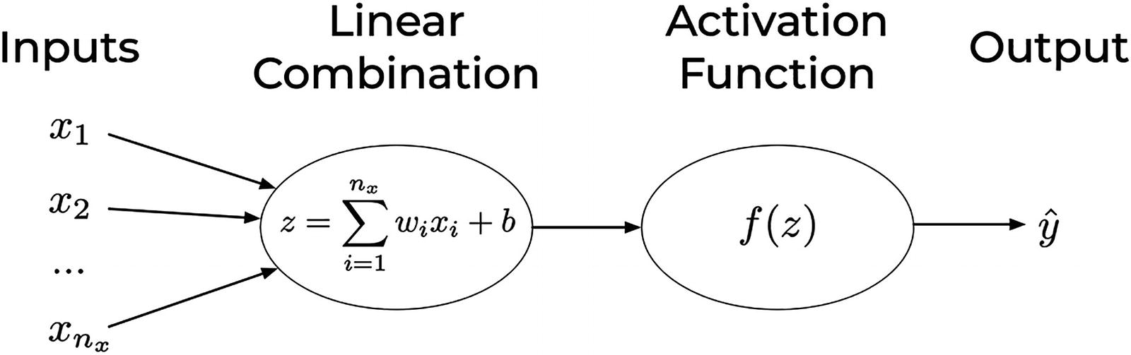
A representation of a single neuron with the operation highlighted. This is also called the computational graph of a single neuron, or in other words, a graphical representation of the operations needed to calculate  from the inputs
The inputs are not placed in a bubble, simply to distinguish them from nodes that perform an actual calculation.
The weight’s names are typically not written. The expected behavior is that before passing the inputs to the central bubble (or node), the inputs will be multiplied by the relative weight. The first input x1 will be multiplied by w1, x2 by w2, and so on.
The first bubble (or node) will sum the inputs multiplied by the weights (the xiwi for i = 1, 2, …, nx) and then sum the result to the bias b.
The last bubble (or node) will finally apply to the resulting value the activation function f.


A simplified version of Figure 2-1. Unless otherwise stated, it is usually understood that the output is  . The weights are often not explicitly reported in the neuron representation
A Short Introduction to Matrix Notation


 as
as
 : Neuron (and later network) output
f(z): Activation function (sometimes called a transfer function) applied to z
w: Weights (vector with nx components)
b: Bias
An Overview of the Most Common Activation Functions
There are many activation functions at your disposal to change the output of a neuron. Remember, an activation function is simply a mathematical function that transforms z in the output  . Let’s look at the most common ones.
Identity Function

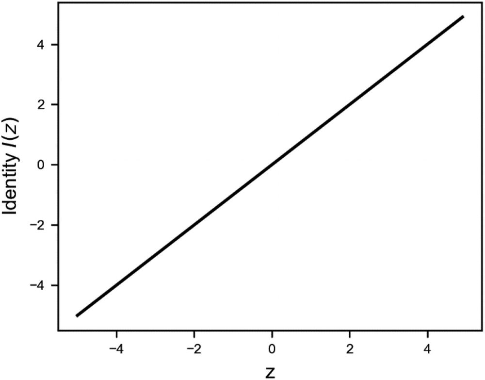
The identity function
Sigmoid Function

It is primarily used for classification models, where we want to predict the probability as an output (remember that a probability may only assume values between 0 and 1).
Note It is very useful to know that if we have two NumPy arrays, A and B, the following are equivalent: A/B is equivalent to np.divide(A,B), A+B is equivalent to np.add(A,B), A-B is equivalent to np.subtract(A,B), and A*B is equivalent to np.multiply(A,B). If you know object-oriented programming, we say that in NumPy basic operations like /, *, + and - are overloaded. Note also that these four basic operations in NumPy act element-by-element (also called element-wise).
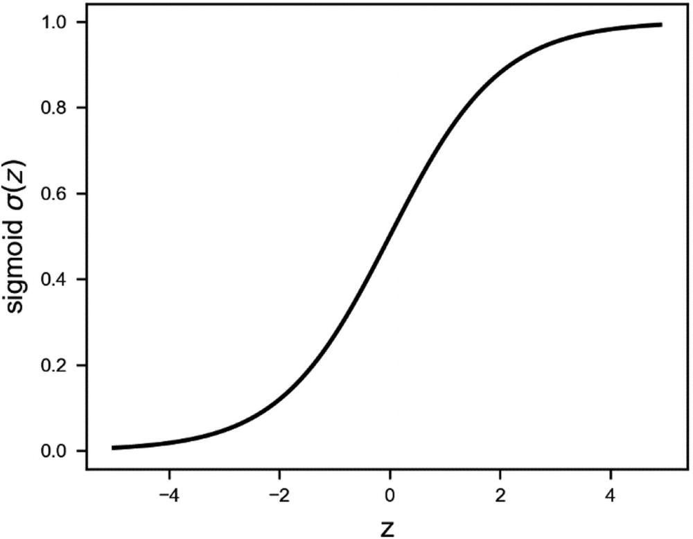
The sigmoid activation function is a s-shaped function that goes from 0 to 1
The sigmoid activation function (that you can see in Figure 2-4) is especially used for models where we must predict the probability as an output, as logistic regression (remember that a probability may only assume values between 0 and 1). Note that in Python, if z is big enough, it can happen that the function returns exactly 0 or 1 (depending on the sign of z) for rounding errors. In classification problems we will calculate logσ(z) or log(1 − σ(z)) very often, and therefore this can be a source of errors in Python since it will try to calculate log0, which is not defined. For example, you can start seeing nan appearing while calculating the cost function (more on that later).
Although σ(z ) should never be exactly 0 or 1, while programming in Python the reality can be quite different. It may happen that, due to a very big z (positive or negative), Python will round the results to exactly 0 or 1. This may give you errors while calculating the cost function for classification, since you need to calculate logσ(z ) and log(1 − σ(z )). Therefore, Python will try to calculate log0, which is not defined. This may happen, for example, if you don’t correctly normalize the input data or if you don’t correctly initialize the weights. For the moment, it’s important to remember that although everything seems under control mathematically, the reality while programming can be more difficult. It’s good to keep this in mind while debugging models that give, for example, nan as a result for the cost function.
Tanh (Hyperbolic Tangent) Activation Function

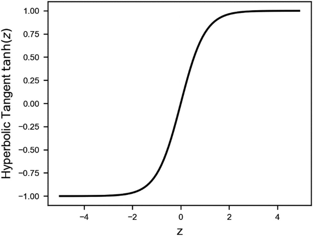
The tanh (or hyperbolic function) is an s-shaped curve that goes from -1 to 1
ReLU (Rectified Linear Unit) Activation Function


It is worth it to spend a few moments to see how to implement ReLU in a smart way in Python. Note that when you start using TensorFlow, it is implemented for you, but it’s still very instructive to see how different Python implementations can make a difference when implementing complex deep learning models.
- 1.
np.maximum(x, 0, x)
- 2.
np.maximum(x, 0)
- 3.
x * (x > 0)
- 4.
(abs(x) + x) / 2
The difference is stunning . Method 1 is four times faster than method 4. The numpy library is highly optimized, with many routines written in C. But knowing how to code efficiently still makes a difference and can have a great impact. Why is np.maximum(x, 0, x) faster than np.maximum(x, 0)? The first version updates x in place, without creating a new array. This can save a lot of time, especially when the arrays are big. If you don’t want to (or can’t) update the input vector in place, you can still use the np.maximum(x, 0) version.
Remember that, when optimizing your code, even small changes can make a huge difference. In deep learning programs, the same chunk of code is repeated millions and billions of times, so even a small improvement can have a huge impact in the long run. Spending time optimizing your code is a necessary step that will pay off.
Leaky ReLU


The Leaky ReLU activation function with α = 0.05. This value has been chosen to make the difference between x > 0 and x < 0 more marked. Smaller values for α are typically used. Testing your model is required to find the best value
The Swish Activation Function


The Swish activation function for three different values of the parameter β
where β is a learnable parameter (see Figure 2-8). Their studies have shown that simply replacing ReLU activation functions with Swish improves classification accuracy on ImageNet by 0.9%, which in today’s deep learning world is a lot. ImageNet is a large database of images that is often used to benchmark new network architectures or algorithms, as in this case, networks with a different activation functions. You can find more information about ImageNet at http://www.image-net.org/.
Other Activation Functions
- ArcTan

- Exponential Linear unit (ELU)

- Softplus

Note Practitioners almost always use only two activation functions: the sigmoid and the ReLU (with probably the ReLU in the lead). With both you can achieve good results. Both can, given a complex enough network architecture, approximate any nonlinear function.3 Remember that when using TensorFlow, you do not have to implement them by yourself. TensorFlow offers an efficient implementation for you to use. But is important to know how each activation function behaves to understand when to use which one.
Now that we briefly discussed all the necessary components, you can use the neuron on some real problems. Let’s first see how to implement a neuron in Keras and then how to perform linear and logistic regression with it.
How to Implement a Neuron in Keras
The Sequential class groups a linear stack of layers into a tf.keras.Model. In this straightforward case, we need just one layer made by a single neuron, defined by the layers.Dense command, which specifies 1 unit (neuron) inside a layer and the shape of the input dataset. The Dense class implements densely connected neural networks’ layers (more on that in the next chapters).
In the next paragraphs, you see two practical examples of how to use this simple approach—choosing the right activation function and the proper loss function—to solve two different problems, namely linear regression and logistic regression.
Python Implementation Tips: Loops and NumPy
As you have just seen, Keras does all the dirty work for you. Of course, you can also implement the neuron from scratch, using Python standard functionalities such as lists and loops, but those tend to become very slow as the number of variables and observations grows. A good rule of thumb is to avoid loops when possible and use NumPy (or TensorFlow) methods as often as possible.
The actual values are not relevant for our purposes. We are simply interested in how fast Python can multiply two lists, element by element. The time reported was measured on a 2017 Microsoft Surface laptop and will vary greatly depending on the hardware that the code runs on. We are not interested in the absolute values, but only in how much faster NumPy is in comparison to standard Python loops. If you are using a Jupyter Notebook, it is useful to know how to time Python code in a cell. To do this, you can use a “magic command.” Those commands start (in a Jupyter Notebook) with %% or with %. It’s a good idea to check the official documentation to better understand how they work (http://ipython.readthedocs.io/en/stable/interactive/magics.html).
The NumPy code needed only 21ms or, in other words, it was roughly 100 times faster than the code with standard loops. NumPy is faster for two reasons: the underlying routines are written in C, and it uses vectorized code as much as possible to speed up calculations on a large amount of data.
Vectorized code refers to operations performed on multiple components of a vector (or a matrix) at the same time (in one statement). Passing matrixes to NumPy functions is an excellent example of vectorized code. NumPy will perform operations on big chunks of data simultaneously, obtaining much better performance than standard Python loops since the latter must operate on one element at a time. Note that part of the excellent performance NumPy shows is also due to the underlying routines being written in C.
While training deep learning models, you will find yourself doing this kind of operation over and over. Such a speed gain will make the difference between having a model that can be trained and one that will never give you a result.
Linear Regression with a Single Neuron
This section explains how to build your first model in Keras and how to use it to solve a basic statistical problem. You can, of course, perform linear regression quickly by applying traditional math formulas or using dedicated functions such as those found in Scikit-learn. For example, you can find the complete implementation of linear regression from scratch with NumPy, using the analytical formulas (see http://adl.toelt.ai/single_neuron/Linear_regression_with_numpy.html) in the online version of the book. However, it is instructive to follow this example, since it gives a practical understanding of how the building blocks of deep learning architectures (i.e., neurons) work.
If you remember, we have said many times that NumPy is highly optimized to perform several parallel operations simultaneously. To get the best performance possible, it’s essential to write your equations in matrix form and feed the matrixes to NumPy. In this way, the code will be as efficient as possible. Remember: avoid loops at all costs whenever possible.
The Dataset for the Real-World Example
Floor (the floor of the house in which the measurement was taken)
County (the U.S. county in which the house is located)
uppm (a measurement of the uranium level of the soil by county)
This dataset fits a classical regression problem well since it contains a continuous variable (radon activity) to predict. The model that we will build is made of one neuron and will fit a linear function to the different features.
You do not need to understand or study the features. The goal here is to understand how to build a linear regression model with what you have learned. Generally, in a machine learning project, you would first study your input data, check its distribution, quality, missing values, and so on. But we skip this part to concentrate on the implementation with Keras.
In machine learning, the variable we want to predict is usually called the target variable.
We have four features (floor, county, log_uranium_ppm, and pcterr) that we will use as predictors of radon activity.
As suggested, we have prepared the data in matrix form. Let’s briefly review the notation, which will come in handy when building the neuron. Normally we have many observations (919 in this case). We use an upper index to indicate the different observations between parentheses. The ith observation is indicated with x(i), and the jth feature of the ith observation is indicated with  . We indicate the number of observations with m.
In this book, m is the number of observations and nx is the number of features. Our jth feature of the ith observation is indicated with  . In deep learning projects, the bigger the m, the better. So be prepared to deal with a massive number of observations.

where each row is an observation, and each column represents a feature in the matrix X that has the dimensions m × 4.
Dataset Splitting
In any machine learning project, to check how the model generalizes to unseen data, you need to split the dataset into different subsets.4 When you build a machine learning model, you first need to train the model, and then you have to test it (i.e., verify the model’s performances on novel data). The most common way to do this is to split the dataset into two subsets: 80% of the original dataset to train the model (the more data you have, the better your model will perform) and the remaining 20% to test it.5
We will use 733 observations to train our linear regression model, and we will then evaluate it on the remaining 186 observations.
Linear Regression Model
Keep in mind that using a single-neuron model is overkill for a linear regression task. We could solve linear regression exactly without using gradient descent or a similar optimization algorithm. As mentioned, you can find an exact regression solution example, implemented with NumPy library, in the book’s online version.

The weights and bias need to be chosen so that that the network output is as similar as possible to the expected target variable.

where the sum is over all m observations. This is the typical loss function chosen in a regression problem. By minimizing L(w, b) with respect to the weights and bias, we can find their optimal values.
Minimizing L(w, b) is done with an optimizer. If you remember from the last chapter, gradient descent is the most basic example of an optimizer and could be used to solve this problem. Since is not available out of the box in TensorFlow, we use the RMSProp optimizer for practical reasons. Don’t worry if you don’t know how it works. Just know that it is simply a more intelligent version of the GD algorithm. You learn how it works in detail in the following chapters.
Keras Implementation
If you have no experience with Keras , you can consult the appendixes of this book. There you will find an introduction to Keras that will give you enough information to be able to understand the following discussion.
First of all, we defined the network structure (also called network architecture) with the keras.Sequential class, adding one layer6 made of one neuron (layers.Dense) and with input dimensions equal to the number of features used to build the model. The activation function is the one set by default, i.e. the identity function.
Then, we defined the optimizer (tf.keras.optimizers.RMSprop), setting the learning rate to 0.001. The optimizer is the algorithm that Keras will use to minimize the cost function. We use the RMSprop algorithm in this example.
Finally, we compile the model (i.e., we configure the model for training), setting its loss function (i.e., the cost function to be minimized), its optimizer, and the metric to be calculated during performance evaluation (model.compile). The function returns the built model as a single Python object.
The learning rate is a very important parameter for the optimizer. In fact, it strongly influences the convergence of the minimization process. It is a common and good behavior to try different learning rate values and observe how the model’s convergence changes.
Thus, we have five parameters to be trained—the weights associated with the four features, plus the bias .
The Model’s Learning Phase
As you can see, training the model in Keras is straightforward. It is enough to apply the fit method to our model object. fit takes as inputs the training data and the number of epochs.

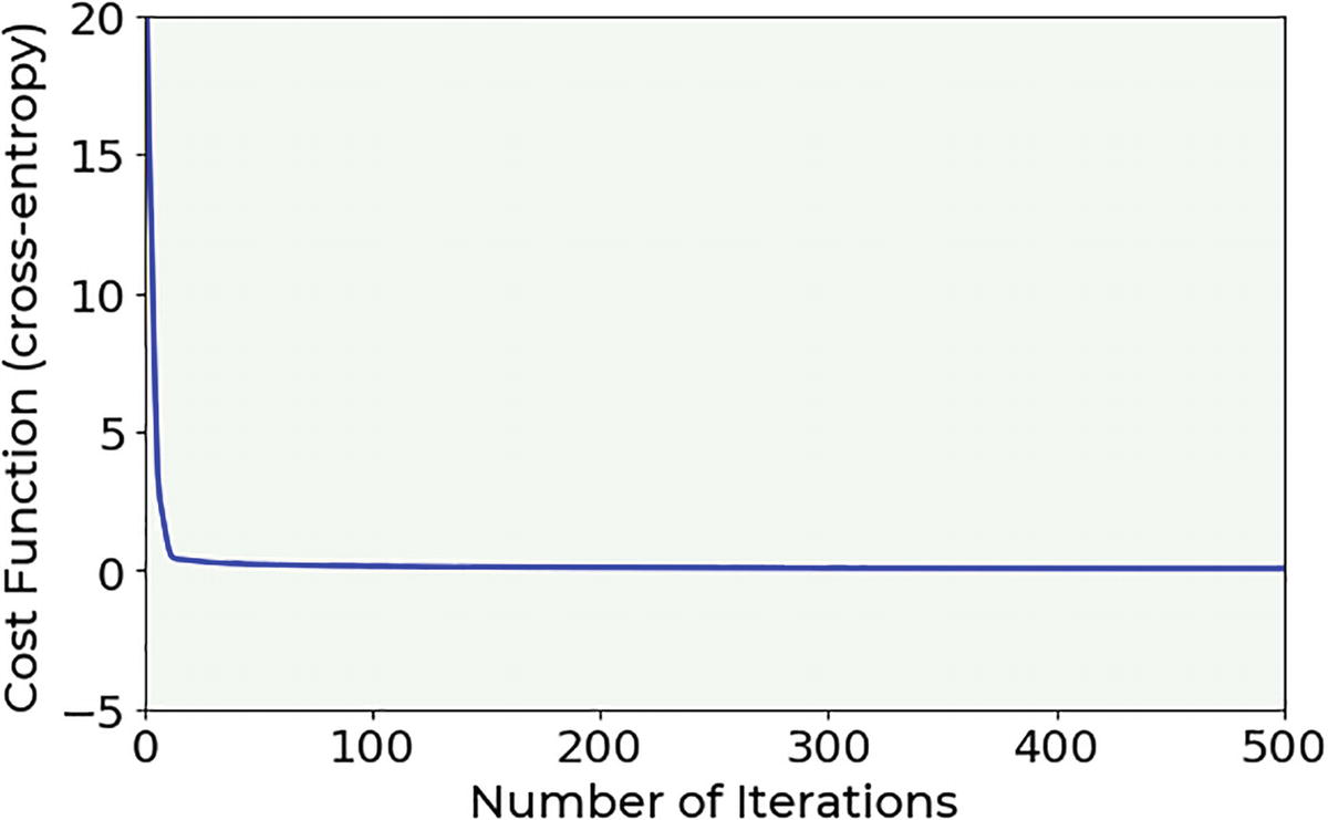
The cost function behavior during the model training, applied to the radon dataset with a learning rate of 0.001
Looking at Figure 2-9, you can see that, after 400 epochs, the cost function remains almost constant in its value, indicating that a minimum has been reached.
Those are the weights we were expecting.
Model’s Performance Evaluation on Unseen Data
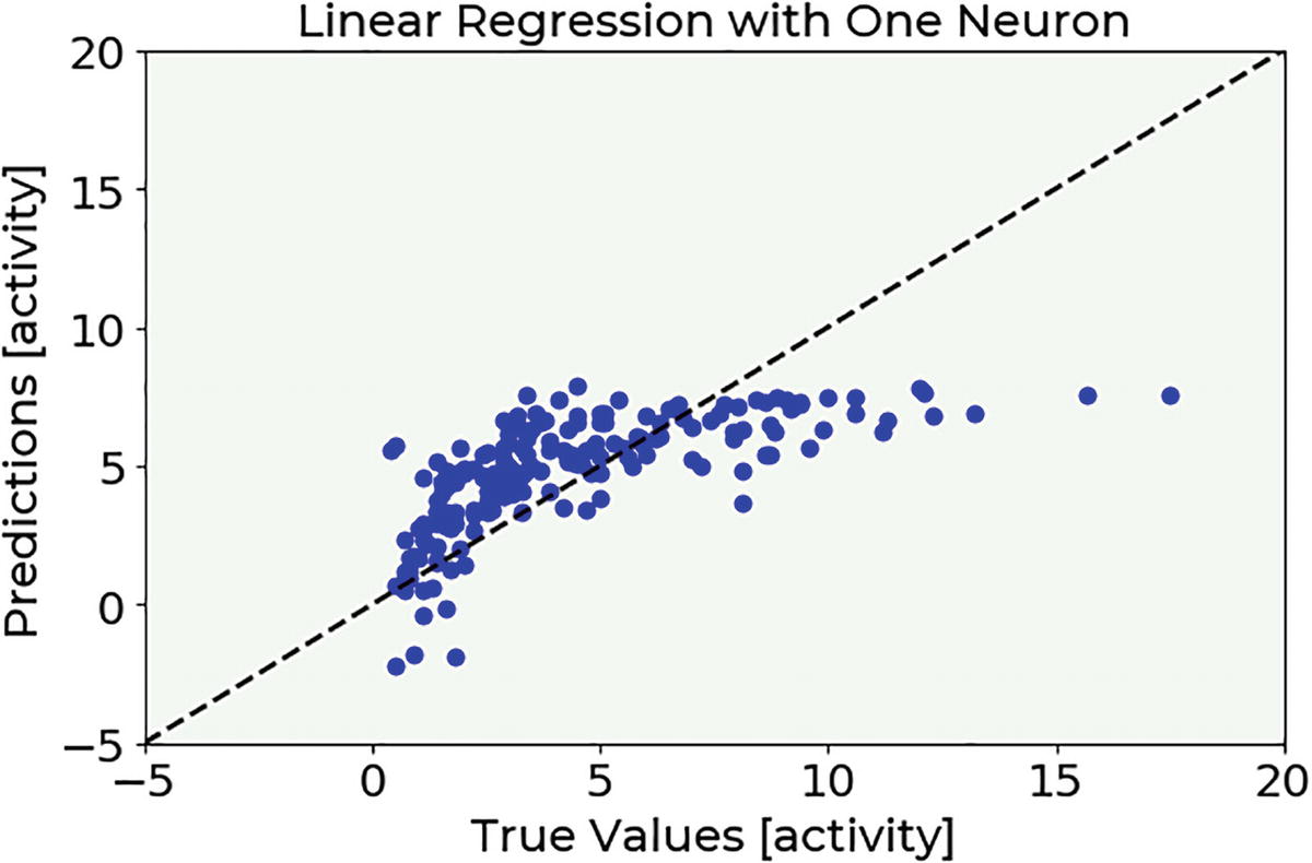
The predicted target value vs. measured target value for our model, applied to our testing data
If you have followed so far, congratulations! You just built your very first neural network, with just one neuron, but still a neural network!
Logistic Regression with a Single Neuron
Now let’s try to solve a classification problem with a single neuron. Logistic regression is a classical algorithm and probably the simplest classification. We will consider a binary classification problem: that means we will deal with the problem of recognizing two classes (that we label as 0 or 1). We need an activation function that’s different from the one we used for linear regression, a different cost function to minimize, and a slight modification of the output of our neuron. The goal is to be able to build a model that can predict if a certain new observation is in one of two classes. The neuron should give as output the probability P(y = 1| x) of the input x to be of class 1. We will then classify our observation as being in class 1 if P(y = 1| x) > 0.5 or in class 0 if P(y = 1| x) < 0.5.
It is instructive to compare this example with the one about linear regression, since they both are applications of the one-neuron model yet are used to solve different tasks. You should pay attention to the similarities and differences with the linear regression model discussed previously. You are going to see how simple using Keras is in this case and how, by changing a few things (such as the activation and loss functions), you can easily obtain a different model that can solve a different problem.
The Dataset for the Classification Problem
As in the linear regression example, we use a dataset taken from the real world, to make things more interesting. We employ the BCCD dataset, a small-scale dataset for blood cell classification. The dataset can be downloaded from its GitHub repository [8]. For this dataset, two Python scripts have been developed to make preparing the data easier. All the code can be found in the online version of the book. In the example, a slightly modified version of the two scripts is used. Remember, you are not interested at this point in how the data looks or how it is cleaned. You should focus on how to build the model with Keras.
- 1.
Red blood cells (RBC)
- 2.
White blood cells (WBC)
- 3.
Platelets
To make it a binary classification problem, we will consider only the RBC and WBC types. The model that will be trained has one neuron and will predict if an image contains an RBC or a WBC type by using the xmin, xmax, ymin, and ymax variables as features.
For simplicity, as in the linear regression example, we will skip all the import and load details and concentrate on the fundamental steps of the code, such as dataset preparation, model creation, and performance evaluation. You can find the complete code on the online version of the book. Note that the greatest differences between this case and the linear regression lie in the chosen activation and cost function.

A sample image from the BCCD dataset
Note that the features we employ in this example are not the pixel values of the image, but the location of the edges of the bounding box of the cell. In fact, for each image, we have only four values (xmin, xmax, ymin, and ymax).
Dataset Splitting
So, we use 3631 observations to train our logistic regression model and then evaluate it on the remaining 896 observations.
Now comes a particularly important point. The labels in this dataset as imported will be 'WBC' or 'RBC' strings (they simply tell you if an image contains white or red blood cells). But we will build our cost function with the assumptions that our class labels are 0 and 1. That means we need to change our train_y and test_y arrays.
When doing binary classifications, remember to check the values of the labels you are using for training. Sometimes using the wrong labels (not 0 and 1) may cost you quite some time in understanding why the model is not learning.
Now all images containing RBC will have a label of 0, and all images containing WBC will have a label of 1.
The Logistic Regression Model
This model will be made up of one neuron and its goal will be to recognize two classes (labeled 0 or 1, referring to RBC or WBC inside a cell image). This is a binary classification problem .


Explaining the cross-entropy loss function goes beyond the scope of this book, but if you are interested, you can find it described in many books and websites. For example, you can check out [7].
Keras Implementation
We have five parameters to be trained in this case as well—the weights associated with the four features plus the bias.
The Model’s Learning Phase
As with the linear regression example, training our neuron means finding the weights and biases that minimize the cost function. The cost function we chose to minimize in our logistic regression task is the cross-entropy function, as discussed in the previous section.
The cost function resulting in our model applied to the BCCD dataset with a learning rate of 0.001
Note that, after 100 epochs, the cost function remains almost constant, indicating that a minimum has been reached.
The Model’s Performance Evaluation

where the number of cases correctly identified is the sum of all positive samples and negative samples (i.e., all 0s and 1s) that were correctly classified. These are usually called true positives and true negatives.
With this model, we reach an accuracy of 98%. Not bad for a network with just one neuron.
Conclusion
This chapter looked at many things. You learned how a neuron works and what its main components are. You also learned about the most common activation functions and saw how to implement a model with a single neuron in Keras to solve two problems: linear and logistic regression. In the next chapter, we look at how to build neural networks with a large number of neurons and how to train them.
Linear and logistic regression are two classical statistical models that can be implemented in many ways. This chapter used the neural network language to implement them and to show you how flexible neural networks are. When you understand their inner components, you can use them in many ways.
Exercises
Try using only one feature to predict radon activity and see how the results change.
Try to change the learning_rate parameter and then observe how the model’s convergence changes. Then try to reduce the EPOCHS parameter and observe when the model cannot reach convergence.
Try to see how a model’s results change based on the training dataset’s size (reduce it and use different sizes, comparing the results).
Try to change the learning_rate parameter and observe how the model’s convergence changes. Then try to reduce the EPOCHS parameter and observe when the model cannot reach convergence.
Try to see how a model’s results change based on the training dataset’s size (reduce it and use different sizes comparing the results).
Try to add to labels to Platelets samples and generalize the binary classification model to a multiclass one (three possible classes).
References
[1] https://spectrum.ieee.org/tech-talk/computing/software/biggest-neural-network-ever-pushes-ai-deep-learning, last accessed 27.12.2017.
[2] R. Rojas (1996), Neural Networks: A Systematic Introduction, Springer-Verlag Berlin Heidelberg.
[3] https://www.tensorflow.org/datasets/catalog/radon, last accessed 09.01.2021.
[4] Lever, Jake, Martin Krzywinski, and Naomi Altman. “Points of significance: model selection and overfitting.” (2016): 703.
[5] Srivastava, Nitish, et al. “Dropout: a simple way to prevent neural networks from overfitting.” The journal of machine learning research 15.1 (2014): 1929-1958.
[6] Bengio, Yoshua. “Practical recommendations for gradient-based training of deep architectures.” Neural networks: Tricks of the trade. Springer, Berlin, Heidelberg, 2012. 437-478.
[7] https://rdipietro.github.io/friendly-intro-to-cross-entropy-loss/, last accessed 10.01.2021.
[8] https://www.tensorflow.org/datasets/catalog/bccd, last accessed 10.01.2021.