Chapter 2
Mathematical Modeling
2.1 Introduction
As was indicated in Section 1.1 in Chapter 1, “mathematical modeling” is used as a principal tool in engineering analysis. It is reasonable to ask “What is mathematical modeling?” Different answers to the question will be given by different people. Our definition of mathematical modeling is that it is “an act of translating back and forth between mathematics and physical situations.”
An analogy to the above definition might be a beautiful melody being developed in the mind of a composer with his or her subsequent expressing this melody in symbolic notes on the stave, as illustrated in Figure 2.1

Figure 2.1 Translation of a melody into music notes—an analogy to mathematical modeling in engineering.
In engineering analysis, however, the role that mathematical modeling plays is significantly more complicated than that implied in Figure 2.1. Figure 2.2 illustrates that mathematical modeling involves most of the tasks stipulated in Stages 2 and 3 of engineering analyses as described in Section 1.4 in Chapter 1.

Figure 2.2 The role of mathematical modeling in engineering analysis.
There are essentially four different forms of math tools available to engineers in their engineering analyses.
2.2 Mathematical Modeling Terminology
We will begin mathematical modeling by reviewing the physical meanings of some of the terminology that is frequently used in engineering analyses. It is important for engineers to relate many of the terms that they encountered in previous mathematical courses with the physical meanings these terms represent in solving engineering problems. In this section, we will learn what roles such common terms as “function” and “variable” play in engineering analysis, as well as the physical meanings of “differentiation” and “derivative” in the analysis. We will also learn what “integration” is in a physical sense, and how this mathematical operation can help in solving many engineering problems.
2.2.1 The Numbers
2.2.1.1 Real Numbers
Real numbers can either be integers or rational numbers—a, b, a/b, and so on, with the numbers a and b being constants. Rational numbers can be integers or fractional numbers.
2.2.1.2 Imaginary Numbers
These are the numbers that are multiplies of square root (−1) and that, along with real numbers, compose the complex numbers. Imaginary numbers do not have physical meaning but they appear in some mathematical expressions and solutions.
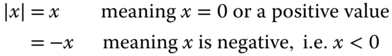
2.2.1.3 Absolute Values
The absolute value of a number recognizes the value (“magnitude”) but not the sign attached to the value. Mathematically, the absolute value can be expressed as
2.2.1.4 Constants
For a constant the value of the number does not change and is always fixed.
2.2.1.5 Parameters
When the value of a number is treated as a “constant” under specific conditions or circumstances we refer to it as a parameter.
2.2.2 Variables
The value of a variable varies with physical conditions, mainly in terms of spatial position or with time. There can be more than one variable involved in engineering analysis.
Two types of variables are commonly involved in engineering analysis:
- 1. Spatial variables. These designate positions in a given space, e.g., (x,y,z) in a space defined by a rectangular coordinate system, or (r,θ,z) in a cylindrical polar coordinate system.
- 2. Temporal variable. The variable representing variation of a physical quantity or system with time t.
Both these types of variables are called “independent variables” because variation of any of these individual variables x, y, and z, or r, θ, z, and t do not affect the values of the other variable presented in the same cases.
2.2.3 Functions
Functions are normally used to represent the physical properties in engineering analyses. Specific functions may be represented with the same symbols used to denote various physical quantities in the analysis. The functions or physical quantities may be represented in mathematical modeling with Latin or Greek letters, according to convention; typical notation includes the following:
- Mass (m), weight (W), length (L), area (A), and volume (V) of a solid.
- Forces applied to a solid (F).
- Temperature (T) of substances, e.g., temperature of a solid or fluid.
- Velocity of a rigid solid body or a fluid in motion (V).
- Distance that a rigid body travels in a straight or curved path (S).
- Stress (σ) and strain (ϵ) in deformed solids.
The typical mathematical expression of functions such as those designating the physical quantities listed above, usually involve associated variables. For example, the function F(x) may represent the physical quantity of force F acting on a beam at a distance x from a reference point. The value of F depends on the value of the variable x in this case.
Change of the value (or magnitude) of function F associated with change in the values of the variable (or variables) of the function can take three different forms.
2.2.3.1 Form 1. Functions with Discrete Values
In general, the value of a function is determined by the values of all variables associated with the function. The values of all the variables may vary independently of all other variables associated with the function. The values of functions with discrete values are determined by the values of discrete variables. For example, in a hypothetical case that involves a family of four (father, mother, and two children) standing on a beam as illustrated in Figure 2.5a, the load to the beam involves four equivalent concentrated forces corresponding to the weights of the members of this family defined by where the individual members stand. The function W(x) represents the loading forces to the beam with the variable x being the location of the beam, at which the load W is accounted for. Thus, the function W(x) has four discrete values W1 at x = x1, W2 at x = x2, W3 at x = x3, and W4 at x = x4 as shown in Figure 2.5b.
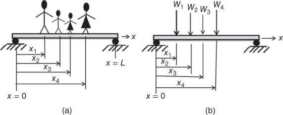
Figure 2.5 Discrete forces applied to a beam structure. (a) People standing on a beam. (b) Equivalent forces applied to the beam.
2.2.3.2 Form 2. Continuous Functions
Because the value of a function is determined by the value of the associated variable or variables, the value of the function can vary continuously with the variation of the associated variable(s), as illustrated in Figure 2.6 for the ambient temperature variation at a place over a period of a day; in the function T will represent the ambient temperature at the time of day, which is denoted by t. The value of the function T(t) varies continuously with continuous variation of the value of the variable t.
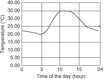
Figure 2.6 Typical diurnal variation of the ambient temperature of a location.
Often a function of discrete values may be approximated by a continuous function if the values of the discrete function are small increments of the associated variable, such as in the case illustrated in Figure 2.7, where the weight W applied to the beam by people standing close together on the beam is as shown in Figure 2.7a. The function representing the equivalent forces W applied to the beam may be approximated by an approximated continuous function W(x) as shown in Figure 2.7b.

Figure 2.7 Discrete and approximated continuous functions. (a) People standing close to each other. (b) Approximate continuous variation of forces.
2.2.3.3 Form 3. Piecewise Continuous Functions
The magnitudes of the physical quantities associated with many physical phenomena in engineering practice vary in ways that can be represented by either continuous functions, as illustrated in Figure 2.6, or by functions of discrete values as illustrated in Figure 2.5. However, there are other cases; one may observe, for example, that the instantaneous water level (y) in the office water cooler tank shown in Figure 2.8 may be represented by both discrete values and continuous variation with the variable time (t). Graphical representation of this physical phenomenon is shown in Figure 2.9, which shows how the water level drops intermittently over time after each serving of water. It illustrates a continuous drop of water level while the release tap is open, followed by a period of constant water level before the next serving.

Figure 2.8 A typical water cooler tank.

Figure 2.9 A qualitative representation of water level in the drinking water tank at different times.
In many cases, functions may involve more than one independent variable, e.g., a function F(x,y), in which the value of function F varies with independent variations of the two independent variables, x and y.
In summary, we observe the following properties of a function:
- 1. Functions are dependent variables themselves because the value of a function changes depending on the values of its associated variables.
- 2. The independent variables are spatial variables or temporal variables, or both.
2.2.4 Curve Fitting Technique in Engineering Analysis
Curve fitting in engineering analysis is undertaken to derive a continuous function that will best fit either a set of data points from experiments or functions with discrete values such as that illustrated in Figure 2.7b. This technique is frequently used to describe the geometric profile of solids in engineering analyses. The continuous functions that are derived using a curve fitting technique can also be used for “interpolation” and “extrapolation” of the value of the function within and outside the range of the variables used in defining this function.
A number of techniques are available for performing curve fitting. Popular techniques used in engineering analysis include (1) least-squares technique, (2) spline curve fitting technique, and (3) polynomial curve fitting technique.
The least-squares curve fitting technique (https://en.wikipedia.org/wiki/Least_square) results in more accurate fitting of large numbers of widely scattered data, whereas the function that is derived using the spline fitting technique (https://en.wikipedia.org/wiki/Spline_(mathematics)) passes through all the data points with smooth transitions. Use of the polynomial function for curve fitting is the simplest of all curve fitting techniques, and will be described in the next subsection.
2.2.4.1 Curve Fitting Using Polynomial Functions
This technique involved the derivation of a polynomial function of order n that will pass through all the given data or sample points. Figure 2.10 shows a data set of five temperatures measured in a production process.
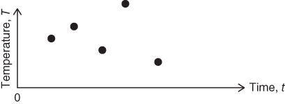
Figure 2.10 Measured temperatures from a fabrication process.
We will use this example to derive a polynomial function that will pass through all measured data points by following a procedure that begins with the assumption of a polynomial function of order n in the general form
in which the order of the polynomial function n = N − 1, with N being the total number of available data (sample) points. The unknown coefficients A0, A1, A2, A3, …, An are determined by a set of simultaneous equations established from the given coordinates of the sample points.
The coordinate system, x–y used in Equation 2.7 is shown in Figure 2.11.

Figure 2.11 Coordinate system for polynomial function curve fitting.
Because the assumed polynomial function in Equation 2.7 is expected to pass through all the sample points with specified coordinates (xi, Yi) as indicated in the right portion of Figure 2.11, the following five simultaneous equations will be established for the five given sample points in Figure 2.10:
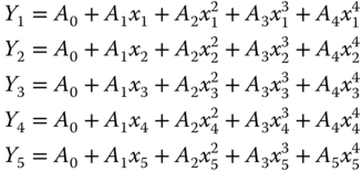
The five unknown coefficients, A0, A1, …, A4 can be determined by solving these five simultaneous equations.
Having obtained this continuous function that includes the three data points, we may use it for interpolating the value of the function between the limits of the sample points, and also for extrapolating for the values outside the limits of the sample range, as illustrated in Figure 2.12.
2.2.5 Derivative
The values of most engineering quantities vary with position in the space, defined by the spatial variables, or/and with time, the temporal variable. For instance, the pressure in a moving fluid varies with position, and it also often varies with time if conditions change.
In most cases, variations of the value of functions occur continuously within the ranges of the associated variables, as illustrated in Figures 2.6 and 2.9.
2.2.5.1 The Physical Meaning of Derivatives
We define a derivative to be the rate of change of the value of a continuous function with respect to one of its associated variables.
Take for example the situation of a pressure chamber used in fabricating a product as illustrated in Figure 2.13. The process requires the product to be subjected to hydrostatic pressure. The chamber can be pressurized by regulating the pumping power and the pressure relief valve of the chamber. The rate of change of the pressure in the chamber varies as illustrated in Figure 2.14 in which the pressure at the closed circle points are the nine measured pressure readings at specific instances from the meter attached to the chamber. The rate of change of the pressure, P of the fluid at time t is expressed mathematically as (ΔP/Δt).

Figure 2.13 A pressurized process chamber.

Figure 2.14 Variation of pressure in the process chamber.
We may observe from the measured pressure in the chamber as shown in Figure 2.14 that the rate of pressure variations represented by ΔP/Δt varies at different time periods Δt at which the measurements of the pressures in the process chamber were taken during the fabrication process. For example, the rate of pressure variation in the period designated Δt2 is ΔP2/Δt2 as shown in the figure. The rate of change of the function P in other periods Δti can be obtained using similar expressions, generalized as
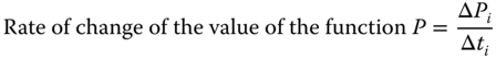
with i = 1, 2, 3, …, 6 in Figure 2.14.
At times the value of a function that represents a physical situation may vary continuously with the continuous variation of the associate variable, such as in the case of the pressure in a pressurized process chamber in Figure 2.13. One may readily conceive that the continuous variation of the pressure P in the chamber with time t cannot be represented by the connection of straight lines of all the measured pressures. The real situation would be more like that represented by the dashed curve in Figure 2.15. The rate of change of the function P can no longer be evaluated by Equation 2.8 because the value of P is changing at all times, not in distinct increments over a finite increment of the variable Δt as was represented in Figure 2.14. A different mathematical expression of P(t) derived by a curve fitting technique such as presented in Section 2.2.4 is thus required.

Figure 2.15 Pressure variations in the process chamber in Figure 2.13.
2.2.5.2 Mathematical Expression of Derivatives
Derivatives are used to evaluate the continuous change of the value of a function with infinitesimally small increments in the associate variables. The increments of the variable are so small that we may use the “approximation” of letting Δt → 0 in our mathematical formulations.
In Figure 2.16 we illustrate the function y with its values “continuously” varying with an independent variable x; expressed mathematically, y = f(x).

Figure 2.16 Continuous variation of a continuous function.
Let us pick two arbitrary points A and B on the curve that graphically represents the function y = f(x). The function's values at these two points are y0 = f(x0) at point A and y1 = f(x1) at point B, where x0 and x1 are the corresponding values of variables associated with function values y0 and y1, respectively.
Let Δx = the increment of the variable x, then the corresponding change of the function values associated with this increment Δx is Δy = y1 − y0 = f(x1) − f(x0). But we also have the relationship x1 = x0 + Δx where Δx is the increment of the variable x as shown in Figure 2.16, which leads to the expression for the corresponding change of the value of the function:
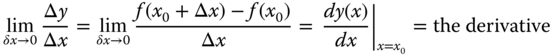
The rate of change of f(x) with respect to x is expressed as
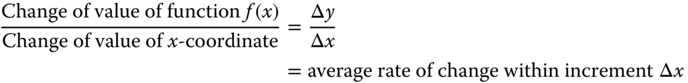
This expression can be interpreted as the rate of change of the value of the function between point A and B in Figure 2.16; alternatively, it is the slope of the curve represented by y = f(x) between point A and B as illustrated in Figure 2.16.
However, it must be realized Figure 2.16 that the average rate change between points A and B is not equal to the exact rate change at intermediate points between the two bounds A and B if Δx is large. The discrepancy becomes smaller with smaller Δx.
A more precise expression for the rate change of function f(x) between x0 and x1 is obtained by reducing the size of the increment Δx. In other words, the rate of change of y = f(x) can be represented accurate only if Δx is very small. The increment Δx is made so small that Δx → 0. This, in reality, means the variation of the function with respective to the variation of x is continuous. Mathematically, it can be expressed as
In general, the derivative of function y = f(x) with respect to the variable x can be expressed in the following ways:

Engineers should realize that not all functions, as represented by y(x) in Equation (2.9), are differentiable. A function is differentiable only if the derivative exists.
Examples of derivatives of functions of various kinds are available in the literature (Ayres, 1964; Spiegel, 1963).
2.2.5.3 Orders of Derivatives
A function, y(x), may be differentiated with its variable x more than once to give various “orders” of derivatives.
The derivative dy(x)/dx in Equation (2.9) is referred to as the first-order derivative of the function y(x), and may be itself a function or a constant.
The derivative of the derivative of the first order (dy(x)/dx)is called the second-order derivative. Mathematically, it is expressed as
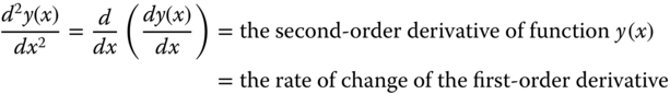
There are also higher-order derivatives for some functions, such as the third- and fourth-order derivatives are shown below:


Engineering analyses, especially mechanical and civil engineering analyses, rarely involve derivatives of higher order than 4.
2.2.5.4 Higher-order Derivatives in Engineering Analyses
Derivatives of a function of different orders have different physical meanings in engineering analysis. Figure 2.17 illustrates a beam in a deflected state due to applied bending loads, with the deflected shape of the beam depicted by the dashed line.

Figure 2.17 A deflected beam subject to bending load.
The following physical quantities required in beam stress analysis are given by derivatives of various orders of the beam deflection at location x, expressed as y(x):

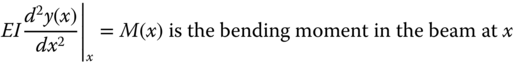
where E and I are the Young's modulus of the beam material and the moment of inertia of the beam cross-section respectively.

The deflection y(x) of a beam of constant cross-section subjected to a distributed load Q(x) can be obtained by solving the differential equation (Equation 2.11):

We will illustrate solving for the deflection and the induced stresses of beams subjected to complex loading and end conditions using Equations 2.10 and Equation 2.11 in a later part of this chapter.
2.2.5.5 The Partial Derivatives
There are engineering problems that involve more than one independent variable in the analysis. The value of the function varies independently with each of the associated independent variables. Figure 2.18 illustrates such a case: that the cantilever beam shown in Figure 2.18a is subjected to a moving load at a variable velocity v(t), where t is the time. Clearly, the load on the beam varies not only with the position x but also with the time t, as expressed in Figure 2.18b.
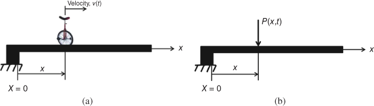
Figure 2.18 A cantilever beam subject to a moving load. (a) Moving load on the beam. (b) The loading function of the beam.
The derivatives of the loading function P given in Figure 2.18b are expressed in terms of each of the two independent variables x and t, but not with both variables included in one derivative. The rate of change of the loading function P needs to be evaluated separately with respect to each of these two variables. We have then two derivatives representing the rate change of the function P(x,t):
and
Note that the differential operators ∂/∂x and ∂/∂t are used in the above derivatives to indicate these are derivatives of a function with respect to the “partial” not the full rate of change of the function values with both variables associated with the function.
2.2.6 Integration
2.2.6.1 The Concept of Integration
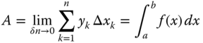
Contrary to differentiation, to obtain the derivatives of functions, which account for the rate of change of the value of a function within selected infinitesimally small increments of the associated variable, integration sums the areas of infinitesimally small elements of area under the graph of the curve y = f(x) with infinitesimally small increments of the associated variable x. Thus, the integral accounts for the total area bounded by the curve defined by the function at x = a and x = b with infinitesimally small increments of variable x, or Δx→0, as illustrated in Figure 2.19, where a and b are the limits of the integration. There are two types of integrals: definite integrals and indefinite integrals. Definite integrals involve a definite range of the associated variable in the determination of the area bounded by the curve y(x) between these limits; indefinite integrals have no specified range of variable in the evaluations.

Figure 2.19 Illustration of the concept of integration.
2.2.6.2 Mathematical Expression of Integrals
Figure 2.20a represents a measured continuous increase of pressure in the process chamber illustrated in Figure 2.13. We denote the pressure increase with time t as P(t). We readily evaluate the rate of the pressure increase at time tk to be![]() according to Equation 2.9. The formula for the area bounded by the curve of function P(t) can be derived by referring to Figure 2.20b.
according to Equation 2.9. The formula for the area bounded by the curve of function P(t) can be derived by referring to Figure 2.20b.

Figure 2.20 Area bounded by a continuous function P(t). (a) A continuous function P(t). (b) The elements of area bounded by P(t).
Referring to the general case of small element k bounded by function y = f(x) in Figure 2.19, the area of the element is Ak ≈ yi−1Δx ≈ ykΔx with yi−1 ≈ yk because the two are located very closely together as Δx→0. The same may be applied to the formulation of element area Ak in Figure 2.20b as Ak ≈ PkΔtk. The total area bounded by the curve of the function P(t) between values of the variable of ta and tb is the sum of all the element areas:

We can see from Figure 2.20b that the rectangular-shaped elements shown in Figures 2.19 and 2.20 will more accurately represent the curve represented by the functions y = f(x) in Figure 2.19 and P(t) in Figure 2.20b as the corresponding increments Δx and Δtk become small; and the true representation of the real continuous functions will be obtained as the increments become infinitesimally small, i.e., as Δx → 0 in Figure 2.19 and Δtk → 0 in Figure 2.20b. Consequently, we have the following expression for the definite integral for continuous functions f(x) (as in Figure 2.19):
Similarly, the integral for the situation depicted in Figure 2.20 can be expressed as
The results of integration of many different forms of functions can be found in references such as Zwillinger (2003).
If we let F(x) be a function whose derivative, F′(x) = f(x), then the function F(x) is an “Anti-derivative” or “indefinite integral” of f(x). Mathematically, this relationship is expressed as

The function f(x) in the integral is called the integrand.
Integration of functions has many applications in engineering analysis. It is used to evaluate areas and volumes enclosed by curves represented by functions. Integration is also used to find geometric quantities such as centroids of plane areas and centers of gravity of solids, as well as moment of inertias for cross-sections of beams and mass moment of inertia of solids involved in curvilinear motion. These geometric properties are frequently involved in many computer-aided design analyses.
2.3 Applications of Integrals
2.3.1 Plane Area by Integration
In Section 2.2.6, we derived the formula for integrals in Equation 2.13 for the area bounded by the curve represented by the function f(x). We will use the same formula for determining the plane areas that can be described by continuous functions.
2.3.1.1 Plane Area Bounded by Two Curves
Integration can also be used to determine areas enclosed by two functions f(x) and g(x) as illustrated in Figure 2.26.

Figure 2.26 Plane area between two curves.
The area defined by the two functions in Figure 2.26 between the limits x = a and x = b is

2.3.2 Volumes of Solids of Revolution
This type of solid has a geometry that is symmetrical about one axis (“the axis of symmetry” in Figure 2.28). It is common in mechanical engineering applications. Typical solids of revolution include cylinders, cones, conical frustums, nozzles, etc. These solids are made up by revolving a plane area about a line, which is often called the axis of rotation.

Figure 2.28 Solid of revolution. (a) Exterior profile of the solid. (b) The same solid with axis of revolution.
Often, engineers need to find the volume of a solid of revolution in order to determine the mass or weight of the solid in many design analyses. The volumes of such solids can be obtained using the special definite integrals described here.
Figure 2.28a indicates a function y(x) that represents the profile of the solid of revolution shown in Figure 2.28b. The gray element of volume shown in Figure 2.28a corresponds in position to the cross-section of the solid normal to the axis of revolution that is shown in Figure 2.28b.
The volume of the solid in Figure 2.28b may be obtained by summing up the volumes of small elements in Figure 2.28a. These elements may be viewed as thin “disks” with radius y(x) and thickness Δx. This is expressed mathematically as
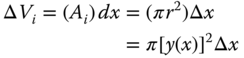
where Ai and r are the cross-sectional area and the radius of the “thin” disk element, respectively.
The volume of the entire solid is the sum of the volumes of all these “thin” disk elements along the axis of revolution, or

in which i designates the disk element number and n is the total number of the disk elements in the subdivided solid.
Because the function y(x) that represents the profile of the solid is a continuous function as shown in Figure 2.28a, we may express the volume of entire solid with the condition that Δx → dx with dx→0. The summation sign in the above expression for the volume V is thus replaced by the integral with the form

The volume of a solid of revolution about the y-axis, such as shown in Figure 2.29, can be determined in a similar manner.

Figure 2.29 Solid volume of revolution about the y-axis.
The area of the shaded element can be expressed as dA = πx2 and the volume of revolution of the shaded element is dv = πx2 dy. The total volume of the solid of revolution about the y-axis can be expressed as

The total volume as computed using the integration method was larger than the 750 cm3 shown in the label of the wine bottle. The discrepancy was mainly due to the discounting of the volume of the “punt” of the wine bottle in the above computation. Figure 2.35 shows the punt of a typical wine bottle.

Figure 2.35 The “punt” at the bottom of a wine bottle.
2.3.3 Centroids of Plane Areas
The centroid of a solid of plane geometry is the point that coincides with the center of gravity of the solid. In engineering analysis, we often consider that the mass or weight of machine components of plane geometry (e.g., a gear or plate) is “concentrated” at the centroid in a typical dynamic analysis of a rigid body of planar geometry in motion (Meriam and Kraige. 2007). Other examples of involving determining the location of centroids of solids of plane geometry include the moving couplers in mechanisms such as illustrated in Figure 2.36. The coupler that is attached to a 4-bar linkage is designed to have its tip A follow a prescribed trajectory with the rotating crank. The induced dynamic force in this oscillating coupler can be a major load to the linkage, and the location of the center of gravity of this coupler of solid plane geometry must be determined in the subsequent stress analysis for the entire mechanism. Figure 2.37 shows an assembly of a mechanism involving a cam and follower that is common in many mechanical systems. The cam, which is usually made in plane geometry, rotates about an axle. The rotary motion of the cam pushes the follower to move up and down according to the profile of the cam. In both of these systems—the coupler of a 4-bar linkage and the cam–follower assembly—rapid motion or rotation of the coupler and the cam is common in practice. The dynamic forces induced by these motions can be significant, and the location of the points of application of force is critical in the design analyses. Identification of the centroids of these planar solids is thus an important part of the design analysis.

Figure 2.36 Mechanism with a coupler.

Figure 2.37 Cam with follower.
A solid of arbitrary plane geometry is shown in Figure 2.38, for which the centroid of the solid plane is located at the coordinates ![]() .
.
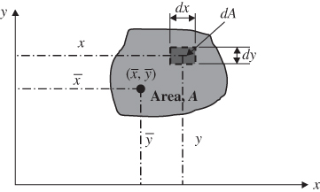
Figure 2.38 Centroid of a plane.
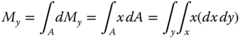
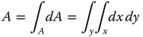
The area of a small element of the plane, such as the one shaded in dark gray in Figure 2.38, is expressed as dA = dx dy. We will define the area moment of the element area dA about the x-axis to be dMx = y(dA) = y dx dy, and the area moment about the y-axis to be dMy = x dA = x dx dy.
The total area moments can thus be obtained by summing the area moments over all area elements in the entire plane solid:
- Area moment about the x-axis:
- Area moment about the y-axis:
2.18b

The coordinate of the centroid of the entire plane can thus be determined by the relations

where the area of the plane is
2.3.3.1 Centroid of a Solid of Plane Geometry with Straight Edges
In the case of solids of plane geometry with at least one straight edge, such as the edge C–D of the plane ABCD shown in Figure 2.39, we may set the straight edge to coincide with one of the coordinates as illustrated in the same figure. The area moments for such case can be expressed as

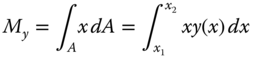

Figure 2.39 Solid of plane geometry with straight edges.
The coordinates of the centroid ![]() of the plane ABCD can be obtained by using Equations 2.21a and 2.21b with the area obtained from Equation 2.20
of the plane ABCD can be obtained by using Equations 2.21a and 2.21b with the area obtained from Equation 2.20
2.3.3.2 Centroid of a Solid with Plane Geometry Defined by Multiple Functions
Cases arise of solids of plane geometry with one edge defined by a multiple functions, such as that illustrated in Figure 2.41. In Figure 2.41, the top edge of the plane is defined by three functions; y1(x), y2(x), and y3(x). One may divide the plane into three regions: A1, A2, and A3. For the corresponding areas of these three subdivisions:
 = the coordinates of the centroid in subdivision A1
 = the coordinates of the centroid in subdivision A2
 = the coordinates of the centroid in subdivision A3
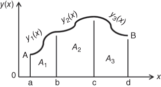
Figure 2.41 Solid of plane geometry with edges defined by multiple functions.
The centroid of the entire plane (ABda), denoted ![]() , may be obtained as the weighted average of those of the three subdivisions as follows:
, may be obtained as the weighted average of those of the three subdivisions as follows:


2.3.4 Average Value of Continuous Functions
Often, engineers need to determine the average value of a function that represents a certain physical phenomenon or quantity. It is not a problem for functions with discrete values. For instance, the average load on a beam in Figure 2.5 can be easily determined by adding the four discrete values of the weights of people standing on the beam and then dividing the total weight by a factor of 4. The answer to the same question for the average value of continuous functions such as those illustrated in Figures 2.6 and 2.15, however, cannot be found by calculating the arithmetic average. Integration of the function between the ranges of the variable is the only method for the purpose.
Take, for example, the continuous function y(x) in Figure 2.43a; the average value of this function over the range x = a and x = b can be determined by
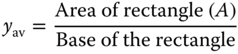
in which area (A) is the area bounded by the function y(x) in Figure 2.43a between x = a and x = b. The same area is equal to the area of the rectangle in Figure 2.43b with the base (b − a). We may thus express the above relationship in the form

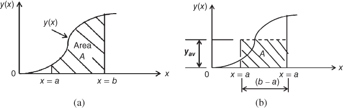
Figure 2.43 Average value of a continuous function. (a) A continuous function. (b) The average value of the function.
2.4 Special Functions for Mathematical Modeling
Engineering students at the junior or senior levels of their undergraduate studies in many engineering schools will already have gained good experience in handling standard functions such as trigonometric and exponential functions in their mathematical education. However, there are engineering analyses that involve situations requiring mathematical formulas to describe physical phenomena that can only be represented by special mathematical functions. These are referred as “special functions” in engineering analysis because they do not appear in many mathematical analyses as commonly as the trigonometric and exponential functions.
There are generally two types of special functions used in engineering analysis:
- Type 1. Special functions appear in mathematical formulations and solutions. We will introduce three common special functions that often appear in solutions of engineering analysis:
-
error function and complementary error functions;
-
gamma function;
-
Bessel functions.
-
- Type 2. Special functions describing special physical phenomena. These functions are useful tools in mathematical modeling of two particular physical phenomena that often present in engineering analyses. We will introduce two such special functions:
- step functions;
- impulsive functions.
2.4.1 Special Functions in Solutions in Mathematical Modeling
2.4.1.1 The Error Function and Complementary Error Function
This function often appears in the solution of differential equations such as diffusion equations. Diffusion is the net movement of a substance (e.g., an atom, ion, or molecule) from a region of high concentration to a region of low concentration and is a common phenomenon in nature. Oxidation of metals in a moist environment is a typical example. We will look at a special case of diffusion analysis in which the variation of the concentration of a solvent, solvent A, with concentration C1 diffuses into another solvent, solvent B, with a lower concentration C2, as illustrated in Figure 2.44.

Figure 2.44 Diffusion of substance A into solvent B.
The concentration of solvent A in the mixed solvent at the depth x and time t after its diffusion into solvent B, expressed as C(x,t), can be obtained using the differential equation already presented in Equation 2.5 (Hsu, 2008):
in which D is the diffusivity of solvent A into solvent B. Diffusivity is a material constant for many substances involved in diffusion processes and the values are available from materials handbooks. The following conditions are specified for the present case of analysis:
where Cs is the concentration of solvent A at the interface of the two solvents and C(∞,t) is the concentration of solvent in the mixed solvent far from the interface at time t.
The solution of Equation 2.5 with the specified conditions is

The function ![]() or erfc(X) with
or erfc(X) with ![]() in Equation 2.24 is called the complementary error function, which is related to the error function erf(X) by the relationship erfc(X) = 1 − erf(X). The error function is given by
in Equation 2.24 is called the complementary error function, which is related to the error function erf(X) by the relationship erfc(X) = 1 − erf(X). The error function is given by

Just as for the sine and cosine functions, the value of the error function erf(x) can be determined from its argument X. Values of the error function with given argument X are available in many textbooks and handbooks (Hsu, 2008; Zwillinger, 2003). It is, however, convenient to recognize that erf(0) = 0 and erf(∞) = 1.
2.4.1.2 The Gamma Function
Like the error function, the gamma function Γ(t) also appears in solutions of mathematical modeling. It takes the form

The gamma function with integer argument t in Equation (2.26) can be evaluated by the simple formulas
The sign “!” designates the “factorial” value of an integer number. Values of gamma functions are available in mathematics handbooks such as Zwillinger (2003).
2.4.1.3 Bessel Functions
Bessel functions are special functions that often appear in engineering analyses involving problems of “circular,” “cylindrical,” and “spherical” geometry. They are named after Friedrich Bessel, a German astronomer and mathematician (1784–1846). Bessel developed the Bessel functions in 1824 from his study of the elliptical motion of planets.
Bessel functions behave in a similar way to the periodic sine and cosine functions except that they oscillate with gradual reduction of both the amplitude and frequency.
Bessel Equation and Bessel Functions
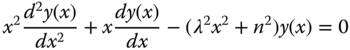
Bessel functions are solutions of the Bessel equation, which has the form
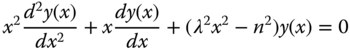
where λ = constant and n = the integers 1, 2, 3,….
The solution of the Bessel equation (2.27) has the form
in which C1 and C2 are arbitrary constants.
The functions Jn(λx) and Yn(λx) are Bessel functions with specific names:
- Jn(λx) is the Bessel function of the first kind of order n.
- Yn(λx)is the Bessel function of the second kind of order n; it is often called a Neumann function.
Figures 2.45a and b illustrate plots of the first two orders of Bessel functions. We will notice that the values of Bessel functions oscillate about the x-axis but with gradual reduction of amplitudes and periods of oscillation.
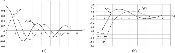
Figure 2.45 Bessel functions. (a) Bessel functions J0(x) and J1(x). (b) The Neumann functions Y0(x) and Y1(x).
A slightly different form of the Bessel equation from Equation 2.27 is
The solution of the modified Bessel equation in Equation 2.29 is
in which In(λx) is a modified Bessel function of the first kind of order n, and Kn(λx) is a modified Bessel function of the second kind of order n.
It may be noted from Figure 2.46 that the modified Bessel functions in Equation 2.30 do not oscillate as do the Bessel functions in Equation 2.28.
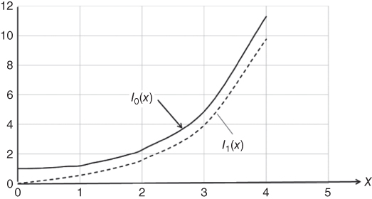
Figure 2.46 Graphical illustration of modified Bessel functions I0(x) and I1(x).
Recurrence Relations of Bessel Functions
One will find that many handbooks offer only the values of Bessel functions of order 0 and 1; Bessel functions of higher orders can be obtained by using the following recurrence relations:
Thus, for example, the value of function J2(x) can be determine by letting n = 1 in Equation 2.31 to get
with the values of J0(x) and J1(x) being available in mathematical handbooks (Zwillinger, 2003).
The modified Bessel functions In(x) and Kn(x) may be related to the Bessel functions by the formulas:
where ![]() .
.
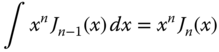
Differentiation and Integration of Bessel Functions
The following expressions are used for differentiation:
and for integration:
2.4.2 Special Functions for Particular Physical Phenomena
2.4.2.1 Step Functions
Step functions originated from “Heaviside step functions.” They are used to describe physical phenomena that come to existence at a given instant in a “time” domain, or at a position in the “space” domain. These physical phenomena remain in their original state thereafter. Physical phenomena of this kind may be a “weight” or “force” existing in a portion of a solid structure, or for the switching on or off of an electric circuit, resulting in the electric current beginning to flow or ceasing to flow in the circuit thereafter.
The physical situation that a step function represents can be represented diagrammatically as in Figure 2.47. The mathematical expression of the step function in Figure 2.47 is

and

Figure 2.47 Graphical description of a step function.
The function ua(x) in Equations 2.36a,b denotes a step function with non-zero values, which begins at x = a. Step functions can be added or subtracted to represent physical quantities existing over infinite range of variables from −∞ < x < ∞ as in Equations 2.36a,b
2.4.2.2 Impulsive Functions
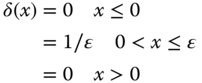
Unlike the step function that describes a physical quantity that comes to existence at a specific time or spatial location and remains at its original value thereafter, the impulsive function is used to describe physical phenomena that exist only for an extremely short period of time or in an extremely small physical extent (i.e., localized physical phenomena). Impulsive functions have other names such as the “delta function” or the “Dirac function.” A graphic representation of this function is illustrated in Figure 2.52.

Figure 2.52 Graphical definition of impulsive function.
The mathematical expression of the impulsive function is

In practice, there is no physical quantity that has an infinite magnitude along with zero pulse width, as illustrated in Figure 2.52. Therefore, for real physical phenomena we deal with finite magnitude and finite but very small pulse width, as illustrated in Figure 2.53. The corresponding function must be modified to be for the following cases.
- a. The pulse occurs at the origin (Figure 2.53):
2.40
- b. The pulse occurs at a point x = a away from the origin (Figure 2.54):
2.41

- where δa(x) is an impulsive function with the pulse located at x = a.

Figure 2.53 Impulse at origin of a coordinate system.
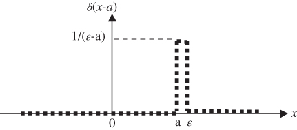
Figure 2.54 Off-origin impulsive function.
The following are some useful properties of impulsive functions in mathematical modeling:


2.5 Differential Equations
We began this book with the statement that “Engineering analysis involves the application of scientific principles and approaches … to reveal the physical state of an engineering system, a machine or device, or structure under study.” This properly reminds engineers that the laws of physics should be used as the basis of all engineering analyses. Consequently, all mathematical modeling in engineering analysis must adhere to the laws of physics.
2.5.1 The Laws of Physics for Derivation of Differential Equations
There are three universal laws of physics that all principles and approaches of engineering analysis must follow:
- 1. Conservation of mass
- 2. Conservation of energy
- 3. Conservation of momentum.
Many “application” laws of physics have been derived from these three fundamental laws of physics. For mechanical engineering analyses, the following application laws are often used as bases for the derivation of differential equations used in engineering analysis such as:
- Newton's laws for the mechanics of solids in static, dynamic, and kinematic analyses of machines and rigid bodies.
- Fourier's law for the conduction of heat in solids (it relates the “heat flows” and the induced “temperature gradients,” or vice versa, in solids).
- Newton's cooling law for convective heat transfer in fluids.
- Bernoulli's law for fluid dynamics.
The following examples illustrate how other laws of physics can be used to derive differential equations in mathematical modeling.
Problems
-
2.1 What is the difference between a real number and an imaginary number, and between a constant and a parameter?
-
2.2 What is mathematical modeling and why does it play a vital role in engineering analysis?
-
2.3 How would you select an appropriate function with appropriate associated variables that could be used in the solution of the following physical problems?
- a. The time required to drain a swimming pool 20 m × 40 m × 2 m deep.
- b. The time required to transport a silicon wafer by a moving chuck from one end to the other end of a platform of given dimensions.
- c. The time required for a large rotor of an electricity generator made of steel to be heated up to 500°C from room temperature in a furnace in a heat treatment process.
- d. The position of your car determined by a GPS (global positioning system).
- e. The amplitude of vibration of a mass attached to a spring after the application of a small but instantaneous disturbance to the initially motionless mass.
- f. The bending stress in a cantilever beam subjected to a concentrated load (also formulate the function and variable representing the bending stress in a diving board over a swimming pool).
-
2.4 Give at least one “real-world” situation that can be represented by (a) function of discrete values, and (b) continuous functions.
-
2.5 Why do we need to use Equation 2.23 to determine the average value of a continuous function?
-
2.6 Use no more than 25 words to outline the application of curve fitting techniques in engineering analysis.
-
2.7 Use no more than 25 words to describe the application of the step function and the impulsive function in engineering analysis.
-
2.8 What are the principal applications of Bessel functions in mathematical modeling of engineering problems?
-
2.9 Describe geometrically the families of lines represented by the following functions: (a) y = mx−3, and (b) y = 4x + b, where m and b are real numbers.
-
2.10 If f(x) = x2−x, show that f(x+1) = f(−x).
-
2.11 Draw the graph of the function
- f(x) = x−1 if 0 < x < 1
- f(x) = 2x if x ≥ 1.
-
2.12 Find the derivatives of each of the following functions:
- a. y = 1/x2
- b. y = (1 + 2x)1/2
- c. y = 1/(2 + x)1/2
-
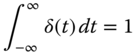
2.13 Derive an expression for the temperature T(r) in a nuclear reactor vessel wall as illustrated in Figure 2.59. The temperature across the reactor wall fits an exponential function with its inner wall maintained at 400°C and the outer wall at 100°C. Constants a and b in Figure 2.59 are the respective inner and outer radii of the wall of the reactor vessel.
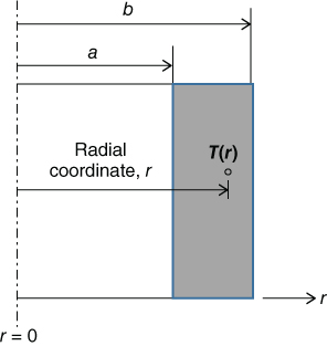
Figure 2.59 Temperature in a nuclear reactor vessel wall.
-
2.14 Find the average ordinate of (a) semicircle of radius r; (b) the parabola = 4 − x2 from x = −2 to +2.
-
2.15 Temperature is measured in either Fahrenheit or Celsius degrees. Fahrenheit (F) and Celsius (C) temperature are related by the expression F = aC + b in which a and b are constants. The freezing point of water is 0°C or 32°F, and the boiling point of water is 100°C or 212°F. (a) Find the equation relating C and F. (b) At what temperature will the temperatures on both scales be equal in value?
-
2.16 Derive a function for the variation of the radius along the length of a tapered metal rod with dimensions shown in Figure 2.60 below:

Figure 2.60 Variation of diameter of a rod.
-
2.17 Find the variation of the cross-sectional area, the volume, and the mass of the tapered rod in Figure 2.60 along its length if the mass density of the rod material is ρ g/cm3.
-
2.18 A common shape of pressure vessel used in industry involves a hollow cylinder covered at both its ends with welded “2:1 elliptical covers” (or “heads”) as illustrated in Figure 2.61. (a 2:1 elliptical head means that the major axis of the ellipse is twice that of the minor axis). Use the integration method to determine the volume content of the pressure vessel with the interior dimensions shown in the figure.

Figure 2.61 A Pressure vessel containing liquid.
-
2.19 An engineer designs a circular filling funnel for a water bottling company with a filling volume of 8 fluid ounces (or 236 cm3). The filling funnel consists of three sections as illustrated in Figure 2.62. Determine the approximate tapering angle θ and the lengths L1 and L2 that satisfy a design constraint on available space that requires L1 + L2 ≤ 10 cm.

Figure 2.62 Optimal design of a three-section funnel. (a) Image of the three-section funnel. (b) Dimensions of the funnel.
-
2.20 Use an integration method to determine the volume content of a square tapered chute as illustrated in Figure 2.63 with dimensions W = 20 cm, H = 10.8 cm, and h = 1.2 cm.

Figure 2.63 Square tapered chute.
2.20 (Hint: You may check your answer with the formula for the volume of a pyramid from handbooks: Volume of 4-side base pyramids V = (base area)(altitude)/3.)
-
2.21 A measuring cup shown in Figure 2.64a has overall dimensions given in Figure 2.64b. Determine the following: (a) the overall volume of the cup; (b) the height L1 for the volume of 200 ml; and (c) the height L2 for the volume of 100 ml.
Figure 2.64 Design of a measuring jug. (a) Image of the measuring jug. (b) The overall dimensions of the jug.
-
2.22 IV bottles such as the one shown in Figure 2.65 are commonly used in hospitals. Use the idealized geometry of the IV bottle shown at the right of the figure to determine
- a. The volume of the liquid in the bottle.
- b. The diameter of the straight portion of the bottle in Figure 2.65 below if the capacity is designed to be 1200 ml (cm3).

Figure 2.65 IV bottle for hospital use.
-
2.23 Use appropriate step functions to describe the loading on the beam illustrated in Figure 2.66.
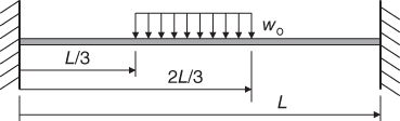
Figure 2.66 A partially loaded beam.
-
2.24 Use appropriate step functions to describe the loading on the beam illustrated in Figure 2.67.
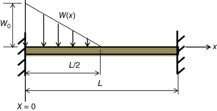
Figure 2.67 Nonuniformly loaded beam.
-
2.25 Use the step function to express the loading function P(x) on a partially loaded beam so that the loading function is valid for the region −∞ < x < +∞. The loading condition on the beam is illustrated in Figure 2.68.

Figure 2.68 Partially loaded beam.
-
2.26 Use an appropriate special function to describe the loading on the beam illustrated in Figure 2.69.

Figure 2.69 A beam subjected to concentrated loads.
-
2.27 Derive a mathematical expression for the distributed loads, P(x) on the beam illustrated in Figure 2.70.

Figure 2.70 A cantilever beam subjected to a distributed load.
-
2.28 Use the integration method to locate the centroid of a flat plate bounded by three corners A, B, and C with the dimensions shown in Figure 2.71.

Figure 2.71 A plate with a curved edge.
-
2.29 Use the integration method to locate the centroid of a plate made of a quarter-circle as illustrated in Figure 2.72.

Figure 2.72 A plate of quarter-circle geometry.
-
2.30 Use the integration method to locate the centroid of a quarter-ellipse as illustrated in Figure 2.73.
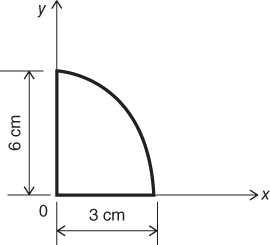
Figure 2.73 A plate of quarter-ellipse geometry.
-
2.31 Use the integration method to locate the centroid of a plate of the geometry and the dimensions shown in Figure 2.74.

Figure 2.74 A plate of geometry bounded by a half ellipse and a half circle.
2.31 Hint: The use of “double integration” technique in determining the enclosed area and area moments of the plane area along both x- and y-coordinates will prove to be a proficient way to reach solutions of this problem
-
2.32 Use the integration method to determine the area and the location of the centroid of a plate coupler of a four-bar linkage similar to that illustrated in Figure 2.36. This coupler plate has dimensions defined by the coordinates of the four corners ABCD as shown in Figure 2.75.

Figure 2.75 Plate coupler of a four-bar linkage.
-
2.33 According to a textbook on dynamics (Hibbeler, 2007), the (mass) moment of inertia (I) of a solid machine component is an important quantity that is used as a measure of the resistance of a rigid body to angular acceleration (α) caused by moment M = Iα, in which the boldface characters indicate vectorial quantities. The mass moment of inertia of a rigid body can be determined by an integral:
a
where r is the perpendicular distance of the moment arm from the axis of rotation, ρ is the mass density of the rigid body, and v is the volume of the rigid body.
2.33 Use the above expression to determine the mass moment of inertia of a flywheel with a linearly tapered profile. The flywheel is made of aluminum with a mass density of 2.7 g/cm3. The cross-section of the wheel is shown in Figure 2.76. Determine the mass moment of inertia of this flywheel using the integral (Equation a) shown above.
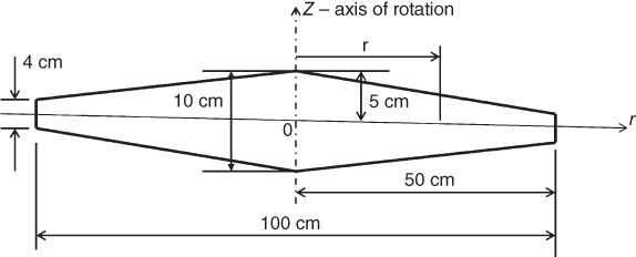
Figure 2.76 Cross-section of a flywheel with a tapered profile.