
Chapter 11
Introduction to Finite-element Analysis
11.1 Introduction
In Chapter 1 we learned the four stages involved in general engineering analyses, with Stage 2 being idealizing actual physical situations for the subsequent mathematical analysis in Stage 3, and Stage 4 being interpretation of analytical results. Idealization of actual physical problems is necessary in most cases of engineering analysis so that analytical tools that engineers have acquired and are available can be used. Idealization of geometry and loading and boundary conditions is frequently carried out in many engineering analyses, and in many of these cases it results in unrealistic solutions from the subsequent mathematical analysis because of possible oversimplification of the real situations in the problems. For instance, in Example 1.2 on the design analysis of a bridge structure some of the assumptions that we made were unrealistic; for example, (1) that the two steel I-beams that support the bridge are “weightless”; (2) that the weight of the bridge surface pavements is also negligible; and (3) that the weight of the passing vehicle is evenly distributed between the front and rear wheels. We made these seemingly unrealistic assumptions in our analysis in order to justify the use of the formula derived from simple beam theory in computing the maximum bending and shearing stresses given in Equations (1.2) and (1.3). This simple analysis with unrealistic idealizations would likely lead to inaccurate analytical results in the maximum bending and sharing stresses that are used to ensure the safety of the bridge structure in meeting the design objectives. Consequently, there was a need to apply “safety factors” to those analytical results in Stage 4 in the interpretation of the analytical results to make up for the deficiency in the analyses that involved unrealistic idealizations of some key physical conditions.
Safety factors (SF) in structural analysis, as we learned in Section 1.6, involve “discounting” the material strength in engineering analysis. For instance, a SF of 4 used in the design analysis of unfired pressure vessels that is stipulated in the design code by the American Society of Mechanical Engineers means that the design analysis utilizes only one-quarter, or 25%, of the strength of the material. This underuse of material strength in engineering analysis results in significant increases in materials and production costs, but such a high safety factor is necessary because of the simple formula used in computing the induced stresses in the vessel and the significant simplification of the structure geometry. The time and effort to determine the required thickness of the pressure vessel become trivial in the design of these unfired pressure vessels using the simple formula available in the design code, and the induced errors in the analysis are made up by this high safety factor.
We thus appreciate that engineers need to achieve proper balance between the use of simple methods in design analyses with unrealistic idealizations to reduce the time and effort required in the analyses and sophisticated analyses with little or no idealization of the real physical conditions. The latter approach obviously requires much more time and resources; the benefit, however, is that it allows engineers to use very low safety factors and thus maximize the use of the material strength in the analysis. The finite-element method presented in this chapter offers such benefits because it is a viable analytical tool for sophisticated engineering analysis for engineers and industry.
A number of excellent books on this subject have been published since the 1970s (Zienkiewicz, 1971; Bathe and Wilson, 1976; Segerlind, 1976; Hsu, 1986; Knight, 1993; Logan, 2017). There have also been many valuable technical papers published in archive journals, conference proceedings, and monographs that deal with the theory and application of this technique, including the very first publication on the principles of the finite-element analysis (Turner et al 1959).
Generally speaking, there are two approaches for developing finite-element analysis. The first is to place emphasis on the accuracy of the result. This approach requires the development of sophisticated algorithms, such as for special elements with higher-order interpolation functions. Most of such work is tailored to special applications. The second approach is to develop commercially available general-purpose programs such as ANSYS, NASTRAN, ABACUS, etc.. Overview of these commercial codes will be presented in the end of this chapter.
Since the purpose of this chapter is to provide readers with an extended overview of this powerful analytical technique, it is necessary restrict coverage of the detailed derivations of the finite-element analysis. Topics such as element library, in-depth treatment of the variational principle, numerical integration schemes, convergence criteria, and so on will be omitted. These topics and detailed derivations of the relevant expressions and equations are adequately covered in the references cited above, and also in the users' manuals of a number of commercial finite-element codes.
This chapter will therefore present only the fundamental principles of the finite-element method. The essence of the discretization concept of the finite-element analysis will be described in Section 11.3. Steps involved in general finite-element analysis will be presented in such a way as to include the formulation of key equations toward the numerical solutions. Readers are expected to develop a firm grip of this technique and its application in various branches of the engineering discipline with the extended overview provided by this chapter.
Mathematical formulations for physical quantities involving multiple components in this chapter will be expressed in matrix forms with the matrix operations described in Chapter 4. Matrices with curvy brackets ({}) will designate the column matrices representing such quantities, and those with square brackets ([]) will designate rectangular matrices. Superscript “T” of matrices designates the transpose of the same matrices.
11.2 The Principle of Finite-element Analysis
The essence of the finite-element method can be summarized in the simple phrase “divide and conquer.” This phrase is often used to describe a strategy for achieving political or military control, which, of course, is not what the finite-element technique intends to achieve. However, the core strategy of the finite-element method is indeed to “divide” the original continuum of complicated geometry with infinite numbers of degrees-of-freedom (DOF) in the solutions into a number of subdivisions of the continuum with specific simple geometry termed “elements.” These elements are interconnected at specific points, either on the sides of the elements and/or at the corners called “nodes” in a discretized model. “Element equations” are derived for each of the elements in the discretized model based on the appropriate physical theories and principles. An “overall structural equation” is then derived by assembling all the element equations in the discretized model, upon which the specified loading and boundary conditions of the original continuum are applied. Desired solutions on the unknown quantities are solved from these “overall structural equations” at every element and nodes using the techniques of solving simultaneous linear equations such as the Gaussian elimination method or its derivatives as presented in Section 4.7.3.
It must be appreciated that the desired solutions are available only at the finite number of elements (and nodes) in the discretized model, not everywhere in the original continuum. In other words, the finite-element method provides solutions only at the elements and nodes of the discretized continuum. It thus reduces the original infinite number of DOF associated with the original continua to a finite number of DOF after the discretization in the finite-element analysis. The concept of “divide and conquer” can thus be viewed as the fundamental principle of this method.
11.3 Steps in Finite-element Analysis
Finite-element analysis (FEA) is now used in many engineering disciplines. It is used to compute stress and temperature distributions in solid structures of complex geometries subject to complicated loading and boundary conditions. It can also be used to predict the pattern of a fluid flowing in channels of complicated geometry. The engineering behavior of solids or fluids with unusual thermophysical and mechanical properties can also be assessed using the FEA. The principles of the application of the FEA in many other engineering disciplines have been illustrated in books such as that of Desai (1979). It is not possible to establish a set of standard procedures for all the computations involved in the problems mentioned. However, as a general guideline, most finite-elements analyses follow eight steps, as will be described below.
Step 1: Discretization of the Real Structures
As already stated, discretization of continua in engineering analyses is the foundation for the formulation of the finite-element analysis. We will present the mathematical expressions that illustrate the principle of the finite-element method by dividing the continuum subjected to the actions of a system of forces, or heat fluxes, or pressures as shown in Figure 11.1a into a number of “elements” of specific geometry interconnected at the nodes (shown as black dots) in Figure 11.1b.

Figure 11.1 Discretization of a continuum subjected to loads. (a) Before discretization. (b) After discretization in a rectangular coordinate system.
By virtue of the actions representing by: ![]() in Figure 11.1a, there exist the induced reactions
in Figure 11.1a, there exist the induced reactions ![]() (such as deflections, strains, stresses) to the applied forces or pressures
(such as deflections, strains, stresses) to the applied forces or pressures ![]() in the case of a stress analysis of solid structures.
in the case of a stress analysis of solid structures.
One may observe that the discretized model in Figure 11.1b offers an approximation to the geometry of the original continuum in Figure 11.1a. One noticeable difference is that the curved boundary of the original medium is now represented by cords of straight edges for the discretized medium in the finite-element analysis.
Figure 11.2 presents a number of commonly used simplex elements in finite-element analysis. Simplex elements are the elements whose physical quantities vary according to linear polynomial functions of the coordinates, and which have the associated nodes at the apexes of the elements.

Figure 11.2 Typical simplex elements.
Of the elements shown in Figure 11.2, the bar element is the simplest form of all elements. It is used in stress analysis of truss structures with long and slender members. Bar elements are also used in beam structures that have similar geometry to the truss members but are able to resist bending loads. Both triangular and quadrilateral elements are used for plate structures with planar geometry. The toroidal elements are used in FE models for axisymmetric solids such as pressure vessels and solids of axisymmetric geometry with cross-sectional areas vary along the axis of symmetry. The elements termed tetrahedral and hexahedral (the former with a geometry similar to a pyramid, but usually skewed in shape, and the latter being six-sided solids with eight apexes) are used to establish FE models for solids of complex three-dimensional geometry such as are illustrated in Figure 11.3.

Figure 11.3 FE model for a three-dimensional solid.
(Courtesy of ANSYS, Inc., Pittsburg, PA, USA)
A major effort in discretizing a continuum for finite-element analysis is involved in registering the discretized FE model to the FE program that has already been installed on the computer. This task requires the user to first set a coordinate system for the discretized model (we will refer to the “FE model” hereafter) and assign numbers following the chronological sequence to all elements and nodes in the model, as in the example of a tapered bar subjected to an in-plane load illustrated in Figure 11.4a. Figure 11.4b is the FE model for the tapered bar with assigned numbers for the 18 hybrid triangular and quadrilateral elements interconnected at 25 nodes. The FE model is situated in an x–y coordinate system, with node 1 being conveniently located at the origin of the coordinates. For illustrative purposes, we let the tapered bar in Figure 11.4a have dimensions of H =8 cm, L1 = 9 cm, L = 18 cm, and r = 2 cm.
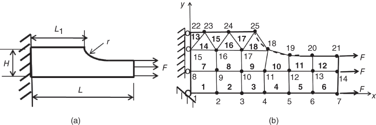
Figure 11.4 FE model for a tapered bar subjected to tensile forces. (a) The tapered bar. (b) An FE model.
Upon finalizing the FE model with the set coordinates for all nodes, the user needs to input the description of nodes to the FE program by entering their coordinates and constraints in displacements and the applied forces as indicated in Table 11.1. Additionally, the user needs to input the element description in terms of the associated nodes of each element in the model, as shown in Table 11.2.
Table 11.1 Nodal description of an FE model of a tapered bar
| Node no. | x-Coordinate (cm) | y-Coordinate (cm) | Nodal constraints in displacements | Applied nodal force |
| 1 | 0 | 0 | ux = uy = 0 | |
| 7 | 18 | 0 | F | |
| 8 | 0 | 3 | ux = 0 | |
| 14 | 18 | 3 | F | |
| 15 | 0 | 6 | ux = 0 | |
| 17 | 6 | 6 | ||
| 18 | 10 | 6 | ||
| 19 | 12 | 4 | ||
| 21 | 18 | 4 | F | |
| 22 | 0 | 8 | ux = 0 | |
| 23 | 1.5 | 8 | ||
| 25 | 9 | 8 |
Table 11.2 Element description of an FE model of a tapered bar
| Element no. | Associated node numbers | Material characterized by input material number |
| 1 | 1, 2, 9, 8 | 1 |
| 6 | 6, 7, 14, 13 | 1 |
| 7 | 6, 9, 16, 15 | 1 |
| 8 | 9, 10, 17, 16 | 1 |
| 12 | 13, 14, 21, 20 | 1 |
| 13 | 15, 23, 22, 22 | 1 |
| 14 | 15, 16, 23, 23 | 1 |
| 15 | 16, 24, 23, 23 | 1 |
| 16 | 16, 17, 24, 24 | 1 |
| 17 | 17, 25, 24, 24 | 1 |
| 18 | 17, 18, 25, 25 | 1 |
One may note from Table 11.1 that not all the nodes in the FE model in Figure 11.4b have been included in the input to the FE program. For example, the coordinates of nodes 2 to 6, and nodes 9 to 13 do not appear in the table. These omissions were possible because these nodes are equally space in the x-coordinates in the FE model, and the FE program is able to interpolate the x-coordinate given the x-coordinates of the two terminal nodes: that is, node 1 and node 7 for all the in-between nodes, and node 8 and node 14 for the x-coordinates of the in-between nodes 9 to node 13. These omissions can significantly lighten the user's effort in inputting the nodal descriptions to the FE program.
The user also needs to input the element descriptions to the FE program as shown in Table 11.2. In this description, the associated nodes of all elements in the FE model need to be specified, as well as the materials of the elements. Since the FE model for the tapered bar in Figure 11.4b consists of hybrid triangular and quadrilateral plate elements, we will include the numbers of all four nodes for the quadrilateral elements, and for all the triangular elements will repeat the number of the last node, as shown in Table 11.2. There is a rule that the numbers of the nodes for each element are presented in counterclockwise order. One will also note from Table 11.2 that descriptions of Element 2 to 5, and Element 9 to 11 are missing in the table. These were omitted because the nodes that are related to these elements are automatically provided by the built-in interpolation of the missing node numbers by the FE program, as with the description of nodes in Table 11.1.
The FE program would thus have full information for the nodes and elements in the user's FE model registered and recorded with the inputs as listed in Tables 11.1 and 11.2.
Step 2: Identify the Primary Unknown Quantities for the Analysis
The “primary unknown” quantity in finite-element analysis is the first, and usually the principal unknown quantity to be obtained in the analysis. The primary unknown will vary from case to case according to the nature of the problem. Frequently used primary unknowns in FE analysis in mechanical engineering include the following:
- Displacements with
 in the elements, in which Ux, Uy, and Uz are the displacement components along the x-, y-, and z-coordinates, respectively.
 - Temperature T in elements in heat conduction analysis.
- Velocity
 in the elements in fluid dynamic analysis, in which Vx, Vy, and Vz are the velocity components along the x-, y-, and z-coordinates, respectively.
Other related unknown quantities, known as the “secondary unknowns” may be obtained from the primary unknown quantity. For example in stress analysis, the primary unknowns are displacements in elements, but the secondary unknowns include strains in the elements that can be obtained by the “strain–displacement relations,” and other secondary unknown quantities such as stresses in the elements can by computed from the element strains using the stress–strain relations, known as Hooke's law, derived from the theory of elasticity.
Step 3: Derive the Interpolation Functions
Interpolation functions in finite-element analysis relate the primary unknown quantities in the elements and those at the associated nodes of a given element. In general, this function is expressed in mathematical form as in Equation 11.1.
where Φ(r) is the primary unknown quantities in the element with r being the position vector representing the corresponding function Φ(x, y, z) in rectangular coordinate system, or (r,θ,z) in cylindrical polar coordinate system. The quantity [N(r)] is the interpolation function in the form of a rectangular matrix and the column matrix {ϕ} is the same primary quantities at the associated nodes of the element.
Interpolation functions such as the ones shown in Equation 11.1 often are referred to as “shape functions” because the form of this function varies with the shape of the elements shown in Figure 11.2. For example, each of the four different shapes of elements in Figure 11.2 has a different number of associate nodes as specified below:
- 1. Tetrahedral elements for 3D solids with 4 nodes
- 2. Triangular plate elements for 2D plane solids with 3 nodes
- 3. Bar elements for 1D solids with 2 nodes
- 4. Axisymmetric triangular elements for solids with circular geometry with 3 nodes
- 5. Other element shapes: hexahedral elements with 6 sides and 8 nodes; quadrilateral plate elements with 4 sides and 4 nodes.
As a result, the interpolation function will have the different forms for the different shapes of elements: three-dimensional function [N(x,y,z)] for tetrahedral and hexahedral elements; two-dimensional function [N(x,y)] for triangular and quadrilateral plate elements; and simple one-dimensional function {N(x)}T for bar elements.
Derivation of interpolation functions is an important step in the finite-element analysis because the primary unknown quantities obtained with the formulations at individual nodes of elements in discretized FE models such as shown in Figure 11.4b must be related to the elements using this function. Besides, the nodes are the points at which all elements in the discretized elements are connected to the effect of the approximation between the original continuum and its discretized geometry, as illustrated in Figures 11.1b and 11.4b. Interpolation functions which relate the solution of primary quantities in individual elements to their associate nodes that serve as “linkages” of all elements in the discretized finite-element model thus play a vital role in the finite-element analysis.
11.3.1 Derivation of Interpolation Function for Simplex Elements with Scalar Quantities at Nodes
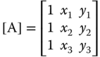
Derivation of interpolation functions for a particular geometry of the elements begins with assumption of a form of the function that describes the variation of the primary quantity in the elements. The simplest function that one may use for this purpose is a linear polynomial function. We will derive such an interpolation function for a relatively simple triangular plate element with three nodes, as illustrated in Figure 11.5 The interpolation function [N(x,y)] that we will derive will relate the primary unknown quantity Φ(x,y) in the element to the same unknown quantity at the associated nodes with set coordinates ϕ1 at (x1,y1), ϕ2 at (x2,y2), and ϕ3 at (x3,y3).
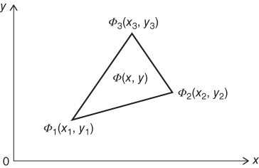
Figure 11.5 Relating element values with those at nodes.
We assume the function that represents the unknown quantity in the element to be a linear polynomial function that has a mathematical form:
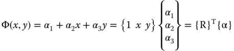
in which the matrix ![]() , and the coefficients α1, α2 and α3 are constants that can be determined by substituting the specified coordinates of the nodal values ϕ1, ϕ2, and ϕ3, to give
, and the coefficients α1, α2 and α3 are constants that can be determined by substituting the specified coordinates of the nodal values ϕ1, ϕ2, and ϕ3, to give
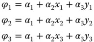
or in a matrix form:
where the matrix
and the inverse of this matrix ![]() is obtained with the result
is obtained with the result

in which the determinant |A| can be evaluated to
where A = the plane area of the triangular plate element
Substituting Equations 11.3 and 11.4 into Equation 11.2, the function Φ(x,y) in the element can be evaluated by the three nodal quantities ϕ1, ϕ2, ϕ3, or {ϕ} to be
The interpolation function, as defined in Equation 11.1 takes the form
where the matrix ![]() and the matrix [h] is given in Equation 11.4.
and the matrix [h] is given in Equation 11.4.
11.3.2 Derivation of Interpolation Function for Simplex Elements with Vector Quantities at Nodes
Primary unknown quantities in triangular plate elements with three fixed nodes in a discretized finite-element model may contain only one component as shown in Figure 11.5. However, in general, they contain two components such as Φx(x,y) along the x-coordinate and for the other component as Φy(x,y) along the y-coordinate, as illustrated in Figure 11.6. Consequently, there are two corresponding components of the same primary quantity at each of the three associated nodes with ϕ1x(x1,y1) along the x-direction and ϕ1y(x1,y1) along the y-coordinate at node 1 situated at (x1,y1), and so on.
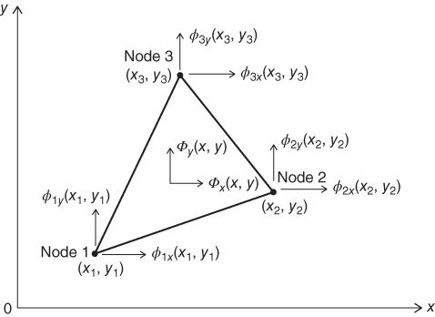
Figure 11.6 Triangular plate element with two unknown components.
According to Figure 11.6, the primary unknowns in the element can be represented by two linear polynomial functions as expressed in Equation 11.7:

where α1, α2, α3, …, α6 are constants to be determined by the nodal values at the specific coordinates of the nodes.
The unknown quantities in the element in Equation 11.7 may be related to those at the three associated nodes as in Equation 11.8:
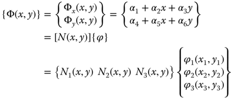
in which N1(x,y), N2(x,y) and N3(x,y) are components of the interpolation function [N(x,y)] associated with the unknown nodal quantities ϕ1, ϕ2, and ϕ3 at nodes 1, 2, and 3 respectively.
We realize that each of the three nodes of the element in Figure 11.6 consists of two components:

By following a similar procedure to that in deriving the interpolation function in the proceeding case, we may derive the three components of the interpolation function, N1(x,y), N2(x,y), and N3(x,y) in Equation 11.8, as in the following expressions (Segerlind, 1976):
where
is the area of the triangular element in Figure 11.6.
Step 8: Solve for Secondary Unknown Quantities
As was mentioned early in Step 2 of finite-element analysis, the selection of primary quantities for the analysis may vary from case to case. For instance, element displacements are denoted as ![]() where Ux and Uy are the two components of the unknown displacement U in the element along the x- and y-coordinate, respectively. These unknown primary quantities in the elements of the discretized model may be related to the quantities at the associated nodes, designated by {ϕ} using the adopted interpolation functions. These unknown nodal quantities are later computed by the overall stiffness equations of the discretized model in Equation 11.18. In reality, however, there is the need to determine other quantities required in the analysis. For instance, in stress analysis of machine structures such as the case illustrated in Figure 11.4, the “stress” and the “maximum stresses” in the structures were required to determine whether the structures would be strong enough to withstand the applied forces F at nodes 7, 14, and 21. We thus need to determine the stress distributions and the magnitude and locations of maximum stress in the structure from the finite-element analysis. The “stresses” and the related “strains” are referred to as the required “secondary unknown quantities” in finite-element analysis.
where Ux and Uy are the two components of the unknown displacement U in the element along the x- and y-coordinate, respectively. These unknown primary quantities in the elements of the discretized model may be related to the quantities at the associated nodes, designated by {ϕ} using the adopted interpolation functions. These unknown nodal quantities are later computed by the overall stiffness equations of the discretized model in Equation 11.18. In reality, however, there is the need to determine other quantities required in the analysis. For instance, in stress analysis of machine structures such as the case illustrated in Figure 11.4, the “stress” and the “maximum stresses” in the structures were required to determine whether the structures would be strong enough to withstand the applied forces F at nodes 7, 14, and 21. We thus need to determine the stress distributions and the magnitude and locations of maximum stress in the structure from the finite-element analysis. The “stresses” and the related “strains” are referred to as the required “secondary unknown quantities” in finite-element analysis.
The secondary unknown quantities can be determined from the primary quantities computed in finite-element analysis by using appropriate laws of physics. For instance, the strain components in the elements may be determined by the element displacement using the “displacement–strain relations” derived in the theory of linear elasticity, and the “element strains” may be related to the element “stress components” by use of Hooke's law. Similar formulations are available for heat transfer analysis, in which Fourier's law of heat conduction and Bernoulli's law for fluid dynamics analysis are frequently used to determine the secondary quantities from the primary unknown quantities obtained from finite-element analyses.
11.4 Output of Finite-element Analysis
Results obtained from finite-element analyses may take different forms, which in general may include (1) tabulated data; (2) contour maps of the computed unknowns in the elements or at nodes; (3) different zones of both the primary and secondary unknown quantities, with different color designations over the input discretized model; and (4) visual animation of selected unknown quantities in the discretized model. Many commercially available finite-element analysis codes such as the ANSYS code have a “post processor” to produce graphic outputs.
Tabulation of output usually includes the user's input of material properties of input elements, descriptions of elements and nodes in the discretized model with specified boundary conditions and loadings, as illustrated in Step 1 of the finite-element analysis. There are, of course, the computed nodal displacements and stresses in all elements. The element stresses in the output are expressed as von Mises stress for multiaxially loaded structures. von Mises stresses are expressed as in Equations 11.21a and 11.21b:
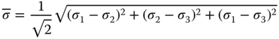
where σ1, σ2, and σ3 are three principal stresses in elements, or the von Mises stress in a solid defined by a rectangular coordinate system of (x,y,z) takes the following form:

in which σxx, σyy, …, σxy, σxz, etc. are the stress components as will be defined subsequently in Section 11.5.1.
von Mises stress is used to show the output stress of elements in finite-element stress analysis because it is regarded as the “effective” stress in multiaxial stress situations, which is frequent in the case of finite-element analyses. Readers will find that the von Mises stress as expressed in Equation 11.21b can be deduced to a single stress component for a uniaxial stress situation with ![]() or
or ![]() , or
, or ![]() in uniaxial stress situations with
in uniaxial stress situations with ![]() .
.
Output in the form of contour maps of the computed unknowns in the elements or at nodes is useful to the users because it offers them the results of the finite-element analysis at a glance. Figure 11.12a shows the isoclinic (principal) stress contours of a gear tooth obtained by a finite-element analysis, with the its discretized model illustrated in Figure 11.12b (Hsu, 1986). The same contours were observed in model testing using a photoelasticity technique. Another useful form of graphic output in of ranges of the unknown quantities in different zones is shown in Figure 11.13.

Figure 11.12 Contour output of a finite-element analysis. (a) Isoclinic stress contour. (b) Finite-element model.
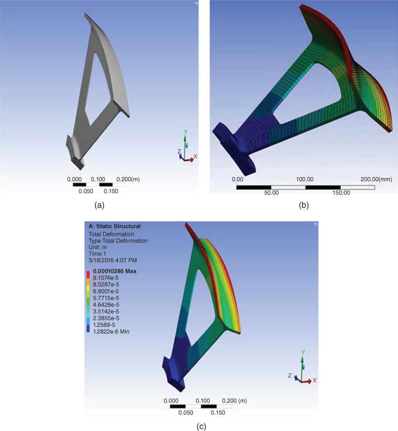
Figure 11.13 Contours of deformation of a wheel section by finite-element analysis. (a) The solid for FE modeling. (b) Deformation with the FE model. (c) Contours of deformation.
(Courtesy of ANSYS Inc., Pittsburg, PA, USA).
Many commercial finite-element analysis codes offer animation of analytical results, such as continuous deformation of a solid structure subject to continuously varying loads. Video clips that record such animation provide great value to users in visualizing the effects on structures in motion, or specific processes in manufacturing or production processes.
11.5 Elastic Stress Analysis of Solid Structures by the Finite-element Method
In this section we will present key formulations for computing induced deformations and stresses in solid structures resulting from externally applied forces. Structural integrity is the number one concern in the design analysis of any machine/device. Finite-element analysis is a valuable analytical tool for stress analysis of machines or devices of complex geometry subject to complex loading and boundary conditions.
The formulations for finite-element analysis presented in this section are excerpts from the author's earlier books (Hsu, 1986; Hsu and Sinha, 1992) Readers are reminded that the physical quantities of multiple components in elastic stress analysis of structures such as displacements, strains, and stresses in deformed solids will be expressed in matrices, and the mathematical operations of the matrices presented in Chapter 4 will be extensively used in deriving the element equations and other formulae in the finite-element analysis.
11.5.1 Stresses
Two physical responses occur in a homogeneous solid with isotropic material properties when it is subjected to a set of applied forces {P} as illustrated in Figure 11.14a. In these responses (1) the solid deforms into a new shape, and (2) the solid develops internal resistance to the applied forces while it deforms into new shapes. The induced internal resistance by the solid eventually reaches a state of equilibrium with the applied forces, and the solid ceases further deformation under this new equilibrium condition.
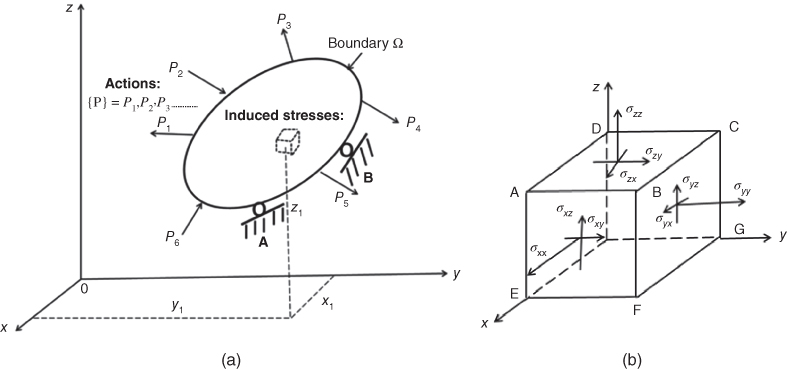
Figure 11.14 Induced stress components in a solid due to external loads. (a) The solid subjected to external loads. (b) Induced stress in the solid.
The intensity of the induced resistance to the applied force in the solid is termed the “stress” at any given location. These stresses may be oriented in different directions in the space defined by the x-, y-, and z-coordinates in Figure 11.14a. The magnitude, location, and orientation of the induced stresses can be denoted by the special notation system described next.
Let us consider an infinitesimally small cubic element located at (x1, y1, z1) with its edges parallel to the three coordinate axes as shown in Figure 11.14b. We envisage that there are six faces of this infinitesimally small cubic element, and there exist stress components with some normal to the faces of the cube, and some others on the faces. A commonly accepted way to denote these stress components is to attach two subscripts to the symbol σ, which denotes the stress magnitude, with the first subscript indicating the coordinate normal to the specific face of the cube, and the second subscript indicating the direction of the stress component. We can thus account for the nine stress components on each of the six faces of the small cubic element inside the deformed solid with the following matrix expression:
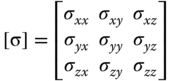
where σxx, σyy, and σzz are the stress components on the faces perpendicular to the respective x-, y-, and z-coordinates, and oriented along the same respective coordinates. We will call these stress components the normal stresses in the deformed solid. The other six stress components with different subscripts—σxy, σxz, and so on—are called shearing stress components; for example, σxy acts on the cube face that is normal to the x-coordinate and points in the y-direction, and σxz is another shearing stress on the same cube face but pointing in the z-direction.
We may account a total of nine stress components on the small cubic element as included in Equation 11.22a. This number is reduced to six in Equation 11.22b via the relationships ![]() , and
, and ![]() because of the new equilibrium condition of the solid in the deformed condition.
because of the new equilibrium condition of the solid in the deformed condition.
We thus have the six independent stress components in deformed solid in three-dimensional stress analyses:
We may also express these stress components in the form of a column matrix in our subsequent derivations:
in which σ1 = σxx, σ2 = σyy, σ3 = σzz , σ4 = σxy, σ5 = σyz, σ6 = σxz
One will note that the stress components with identical subscripts are the normal stresses, whereas those with different subscripts are the shearing stresses.
11.5.2 Displacements
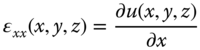
The change of shape of the solid due to externally applied forces is illustrated in Figure 11.15, in which the change of the positions of the points inside and on the boundary of the solid is represented by the movement of point P1 at position (x,y,z) before the loading to point P2 at a new location (x + u, y + v, z + w) after the deformation. The net movement of point P1 to P2 is represented by a vector U with components u, v, and w along the coordinates x, y, and z, respectively. The displacement vector of a point located at r(x,y,z) can thus be expressed as
where the bold-face r is the position vector representing the coordinates as defined in Chapter 3.
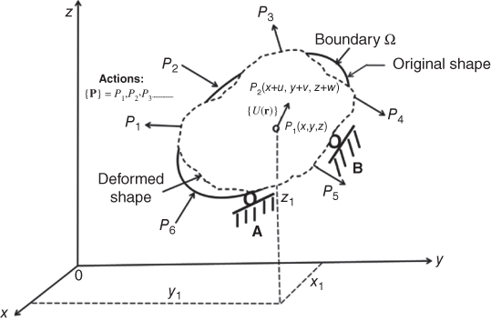
Figure 11.15 Displacements in a deformed solid.
11.5.3 Strains
As we have defined stress in a deformed solid to be the intensity of internal resistance by the solid induced by applied forces, it is appropriate to define the induced strain to be the rate of change of displacement of the solid. Like stresses, strain components can be classified as normal strain components and shearing strain components. However, the reader should bear in mind that normal strain components result in changes in dimensions (and thus the size) of the solid, whereas the shearing strain components cause change only of the shape of the solid, which change is given by the angles of the sides of the cubic faces of the cubic element, which is 90° in the undeformed cubic element before the deformation and the angles between the same faces after the deformation, with a unit of “radians.” Strain components are usually expressed as column matrices corresponding to the six independent stress components, as show in Equation 11.25:
with ϵ1 = ϵxx, ϵ2 = ϵyy, ![]() = ϵzz, ϵ4 = ϵxy, ϵ5 = ϵyz, ϵ6 = ϵxz.
= ϵzz, ϵ4 = ϵxy, ϵ5 = ϵyz, ϵ6 = ϵxz.
11.5.4 Fundamental Relationships
The three essential physical quantities of stress, strain, and displacement in stress analysis of solid structures are mutually interrelated by mathematical expressions derived from the theory of elasticity. We will present only those formulations that are relevant to the subsequent derivations of equations and formulae required for finite-element analysis.
11.5.4.1 Strain–Displacement Relations
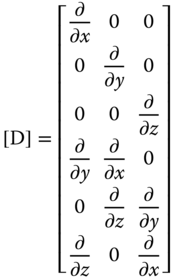
As illustrated in Figure 11.15, the displacements {U(r)} from point P1 at (x,y,z) to point P2 at (x + u, y + v, z + w) with ![]() for the net movement of the point along the x-coordinate,
for the net movement of the point along the x-coordinate, ![]() for the net movement of the same point along the y-coordinate, and
for the net movement of the same point along the y-coordinate, and ![]() for the net movement of the point along the z-coordinate. As we have defined the strain components that account for the rate of change of the displacements along the coordinates that define the deformed solid, and the strain components that exist in the same cubic element as stresses in Figure 11.14b with
for the net movement of the point along the z-coordinate. As we have defined the strain components that account for the rate of change of the displacements along the coordinates that define the deformed solid, and the strain components that exist in the same cubic element as stresses in Figure 11.14b with ![]() ,
, ![]() ,
, ![]() ,
, ![]() ,
, ![]() , and
, and ![]() , we may relate the various strain components to the related displacement components as shown in the following equations:
, we may relate the various strain components to the related displacement components as shown in the following equations:


The relationships in Equations 11.26a to 11.26f may be expressed in the following matrix form:

We may further condense the relationship in Equation 11.27 into the following form for the subsequent derivation of element equations:
where matrix [D] takes the form shown in Equation 11.29 and the element displacement matrix {U} is given in Equation 11.24.
11.5.4.2 Stress–Strain Relations
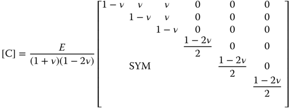
In Figure 11.14 we represented the six independent stress components existing at any point (represented by infinitesimally small cubic elements in the figure) located at (x,y,z). We realize that there are equal numbers of corresponding strain components associate with these stress components. The relationship between these stress and strain components can be expressed by the generalized Hooke's law, as given, fore example, in Hsu (1986). Equation 11.30 shows the matrix form of such a generalized Hooke's law:

or in a compact form:
in which E is the Young's modulus and ν is the Poisson's ratio of the material. The matrix [C], called the elasticity matrix, has the form:
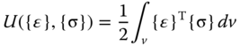
11.5.4.3 Strain Energy in Deformed Elastic Solids
The above formulations are derived from a postulate that in elastic solids, the deformations, stresses, and strains induced by external forces applied to the solid in the equilibrium state will disappear altogether after removal of the applied forces. This postulate implies that there must be a mechanism that restores the solid to its original state after removal of the applied loads. This mechanism is referred to as the “strain energy.” This energy is induced in the solid during the deformation process, and it is “stored” in the deformed solid at the equilibrium state of the solid under external loading. It will be released to restore the deformed solid to its original state upon removal of the applied actions. Since this energy is created by the deformation of the solid expressed by the strains induced by the externally applied forces in the form of the induced stresses, we may mathematically express this energy in the following form:

or in a compact version:
11.5.5 Finite-element Formulation
We will follow the formulations described in Step 5 of Section 11.3 in deriving the element and overall stiffness equations for stress analysis of elastic solid continua. Figure 11.16 illustrates how a cam-shaft assembly may be discretized by a finite number of tetrahedral elements interconnected at nodes. These elements are typically used for discretization of solids with complicated geometry in three-dimensional finite-element analyses. Shapes of these elements are illustrated in Figure 11.2.
Figure 11.16 Finite-element model of a cam-shaft assembly.
(Source: Hsu and Sinha, 1992.)
It was mentioned earlier that hexahedral elements are commonly used in the finite-element modeling of solids of complicated geometry in three dimensions, but since each hexahedral element can be subdivided into four or five tetrahedral elements in actual computations, we will present the subsequent finite-element formulations in terms of typical tetrahedral elements. As illustrated in Figure 11.17, tetrahedral elements have shapes that are similar to pyramids with four apexes (or nodes) for each element. These nodes may be designated by nodes i, j, k, and m as indicated in Figure 11.17.
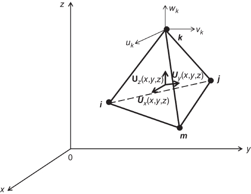
Figure 11.17 Typical tetrahedral elements.
The primary unknown quantity in typical finite-element analysis in stress analysis is the displacements of the element U(r) with r being the position vector in a discretized model representing the coordinates of the solution point (usually located at the center of gravity) in the element. The element displacement vector is expressed as U(x,y,z) in the finite-element formulation.
The displacement in a deformed solid is a vector quantity with components along the three coordinates that define the space in which the element is situated. Mathematically, we may represent the element displacement as

for the element, in which the components Ux, Uy, and Uz along the coordinates x, y, and z are often denoted by U(x,y,z), V(x,y,z), and W(x,y,z), respectively.
The discretization process in the finite-element analysis requires a relationship between the displacements in the element and those at the associated nodes according to Equation 11.1 or as expressed in Equation 11.35 for the current situation:

for the element displacement in a discretized finite-element model with {u} being the displacement components of the associated nodes at fixed coordinates in the discretized model. N(x,y,z) is the interpolation function for the tetrahedral element in Figure 11.17. The displacement components at each of the four nodes of the element in Figure 11.17 consist of three components as in the following:
These nodal displacements are point values in the form of real numbers. The total number of displacement components of the four nodes of a tetrahedral element in Figure 11.17 is thus equal to 12, as expressed in the following matrix form:
where the subscripts identify the nodes: for example, the subscripts i, j, k, and m denote nodes i, j, k, and m, respectively. The notations u, v, and w in Equation 11.36 represent the displacement components along the x-, y-, and z-directions, respectively.
Referring to the tetrahedral element in Figure 11.17, Equation 11.35 can be expanded to give
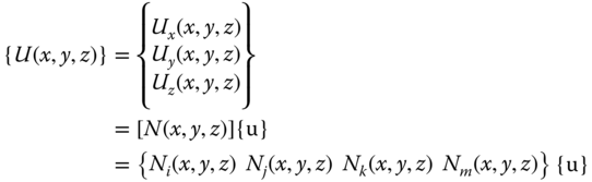
or, in an compact form:
where Ni, Nj, Nk, and Nm are the components of the interpolation function associated with node i, j, k, and m, respectively, in Figure 11.17.
Substituting Equation 11.35 into Equation 11.28 results in the relationship between the element strains and nodal displacements:
where the matrix [B] has the form:
The above expression indicates that the matrix [B(x,y,z)] may be obtained from the derivatives of [N(x,y,z)] with respect to the coordinates x-, y-, and z-, respectively. The matrix [D] is given in Equation 11.29.
The element stresses and the nodal displacement components are related by substituting Equation 11.38 into Equation 11.31 to give Equation 11.40:
And finally, the strain energy in the element is obtained by substituting Equations 11.38 and 11.40 into Equation 11.34, resulting in the following equation for the strain energy of the deformed element:
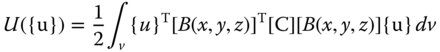
The strain energy U({u}) in Equation 11.41 is the energy stored in the deformed solid (in the elements in this case). It is induced by the deformation of the elements in a discretized finite-element models by the applied forces at the nodes of the elements.
Strain energy in the deformed elements constitutes an important part of the potential energy of discretized solid continua such as shown in Figure 11.1b. The potential energy in a deformed solid is the difference between the induced strain energy in the deformed solid and the work done on the solid by applied external forces. For a continuum such as shown in Figure 11.1a, this difference should be zero; or conversely, the induced strain energy in the deformed solid should be equal to the work done on the solid by the applied forces. In the discretized solid model consisting of individual elements such as that illustrated in Figure 11.1b, however, the equality of the induced strain energy in elements U{u} in Equation 11.41 and the work performed on the same element by applied forces on the surface in the form of surface tractions {t} and body forces {f} may likely not hold. To ensure that the discretized solid is stable and in mechanical equilibrium, such a difference must be kept to a minimum.
The formulation of the potential energy (Π) in a deformed discretized model such as shown in Figure 11.1b can thus be expressed mathematically in the form
where the work produced by applied forces in the deformed element by the body forces {f} and surface tractions {t} can be expressed as
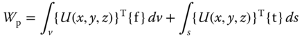
in which {U(x,y,z)} are the displacement components of the element, v and s are the respective volume and surface of the element, and {f} and {t} are the respective body force components and surface tractions applied to the element.
The potential energy in the element can thus be expressed in terms of nodal displacement with the interpolation function [N(x,y,z)] in the following expression:

By applying the principle of variational calculus, the potential energy function in Equation 11.42 has either a maximum or minimum value by solving the following equation:
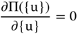
with nodal displacement components {u} to be “point values” which are independent to the coordinates in differentiation. This variation will thus lead to the following equality:

One may also demonstrate the second-order derivative of the potential energy function Π({u}) to be positive:
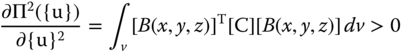
We may thus ensure that the solution of the induced nodal displacements {u} by applied loads as obtained from Equation 11.43 will result a minimum value of the potential function in Equation 11.42.
Equation 11.43 may be expressed in the following form, called the “element equations”:
in which

with the matrix [B(x,y,z)] as in Equation 11.39 and the matrix[C] available from Equation 11.32. The matrix {p} has the form:

and the matrix [N(x,y,z)] is the interpolation function defined in Equation 11.1
In a strict sense, a deformed solid is in equilibrium only when the potential energy Π in Equation 11.42 in all elements in the discretized model is minimum. Consequently, we postulate that the potential energy of the entire discretized solid can be obtained by the summation of potential energies in all individual elements in the discretized solid. This postulate legitimizes our using the following equation for the entire discretized structure:
where

with

as in Equation 11.45; M is total number of elements in the discretized model, and {p} represents the total nodal forces as expressed in Equation 11.46.
The assembly of the element stiffness matrices for the overall stiffness matrix in Equation 11.47 entails following the rule stipulated in Step 6 in Section 11.3 and illustrated in Example 11.3.
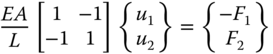
11.5.6 Finite-element Formulation for One-dimensional Solid Structures
We will derive the element equation of a bar element such as shown in Figure 11.7 in Example 11.1 to illustrate the general procedure for developing finite-element formulations.
We will begin by referring to the bar element illustrated in Figure 11.7, made of a material with Young's modulus E. We locate the bar element in a plane defined by the x–y coordinate system as shown in Figure 11.18.

Figure 11.18 An axially deformed bar.
The interpolation function [N(x)] that relates the displacement in the bar element to its two nodes may be derived from a simple polynomial function as we did in Example 11.1. This function has the form shown in Equation (11.10):

The matrix [B(x)] that relates the element strain and the nodal displacement may be obtained using Equation 11.39:

Since the bar element is subjected to two applied forces with –F1 at node 1 and +F2 at node 2 and both these forces act along the longitudinal direction, that is, along the x-coordinate of the bar, the only induced stress component in the bar is σxx along the x-coordinate. Likewise, the only induced strain component is ϵxx along the same direction. The relationship between the induced stress and strain obeys Hooke's law with ![]() where E is the Young's modulus of the bar material. We thus obtain the elasticity matrix [C] = E.
where E is the Young's modulus of the bar material. We thus obtain the elasticity matrix [C] = E.
By substituting the above expression for [N(x)] from Equation 9.10, [B(x)] in Equation 11.49, and with [C] = E and ![]() , where A is the cross-sectional area of the bar element and
, where A is the cross-sectional area of the bar element and ![]() into Equations 11.42 and (11.43), we obtain the element stiffness matrix from Equation 11.45:
into Equations 11.42 and (11.43), we obtain the element stiffness matrix from Equation 11.45:

The nodal forces matrix in this case is
From Equation 11.44 the element equation of the bar element thus has the form
11.6 General-purpose Finite-element Analysis Codes
The incredible versatility of the finite-element method in solving complicated but closer to real engineering problems has resulted in wide acceptance of this method by members of the scientific and engineering communities for handling a great variety of problems with great accuracy and reliability well beyond the capabilities of traditional analytical tools. The broad acceptance of this method has also prompted the commercialization of finite-element analysis software package, or “codes” by a number of reputable companies. Finite-element analysis codes such as ANSYS, ABACUS, COSMOS, and others have served the industry well in the past half a century. Updated versions of these codes with improved accuracy and expanded capabilities were made available to users continually. It is not possible to describe here all of these commercially available codes: what will be presented in this section is merely an overview.
11.6.1 Common Features in General-purpose Finite-element Codes
Finite-element programs that can be used to solve a large class of engineering problems go under the generic name of “general-purpose programs.” Common desirable features of such a program are described below.
- 1. The program should offer extensive capabilities of solving engineering problems ranging from static and dynamic elastic to elastoplastic stress analysis of solid structures made either of traditional materials or of unusual materials such as composites, biomedical materials, and so on, with applied loads from nontraditional sources such as piezoelectric and electrostatic forces as well as molecular forces in the stress analysis of structures at micrometer and nanometer scales.
- 2. It must have a large element library with many more element types to choose from than the simplex elements offered in Figure 11.2. There are other types of elements that can make the finite-element analysis more efficient in terms of setting discretization models and that produce more accurate analytical results. Figure 11.21 shows some of these elements available in the element library of the ANSYS code (Lee, 2015). One will observe from Figure 11.21 that the first of the three listed types of elements is for beam structures using bar elements and the second and third types are for modeling plates of planar geometry. Thin-shell elements are available for structures such as pipes and pressure vessels. One may also note that the last six types of elements have additional nodes at the middle of the edges of the elements. These are the elements normally called the “serendipity” elements, with many such elements having additional nodes on selected locations along the edges of the elements (Bathe and Wilson, 1976; Hsu, 1986). The functions that represent the variation of the primary unknowns in these elements are higher-order polynomial functions, such as the Lagrange polynomials. There are many advantages of using these elements and high-order polynomial interpolation functions, with one obvious advantage of better fitting the element shapes to solids of curved geometry. The higher order of the polynomial functions used in the computations can yield more accurate results from the analyses. The additional nodes in the elements may result in the use of fewer elements in the discretized model for the finite-element analysis. There are many other types of elements that are often offered by general-purpose finite-element codes, such as “spring elements,” “contact elements,” and “interface elements” with unusually large aspect ratio (defined as the ratio of the longest to shortest edges of the element). Other special elements may include the “birth and death elements,” such as are found in the element library of the ANSYS code. These elements are used for cases simulating the “growth” of solid substances involving welding, or the “disappearance” of solid substances such as in etching of structures in microfabrication process, or the growth and propagation of cracks in solid structures in fracture mechanics analyses.
- 3. The package must have user-friendly pre-processor with sufficient versatility. A good pre-processor should include, in addition to extensive material database, easy-to-use automatic mesh generation for users to establish the required discretized model with user-selected density and configurations of finite-element meshes, such as illustrated in Figures 11.3 and 11.13b.
- 4. It must have a comprehensive and easy-to-use post-processor that can display the results of the analysis with visual outputs, either in static graphical form or in animated graphical output for continuous action if so desired. Users should be offered ample options in choosing the desired form for outputs of their analyses.
- 5. It is desirable to offer cost-effective ways to use the code in terms of minimal effort in learning the use of the code, minimal human input, and high computational efficiency. Most commercial finite-element codes adopt highly efficient solution methods.
- 6. Effective interfacing of computer-aided design (CAD) with the finite-element analysis (FEA) is also a desirable feature of general-purpose FE code. It allows the user to perform finite-element analysis using the imported solid model geometry from a CAD package. Figure 11.22a shows a solid model of a coupler from a computer-aided design package to be automatically translated to the ANSYS code for finite-element stress analysis; and Figure 11.22b shows the variation of deformation of the structure under applied load. There are also codes that offer interfacing of CAD/FE with computer-aided-manufacturing (CAM), with the solid models of structures being downloaded to a CAM package ready for mechanical analysis as well as coding for computer-numerically controlled (CNC) machine tools after satisfactory finite-element analysis.
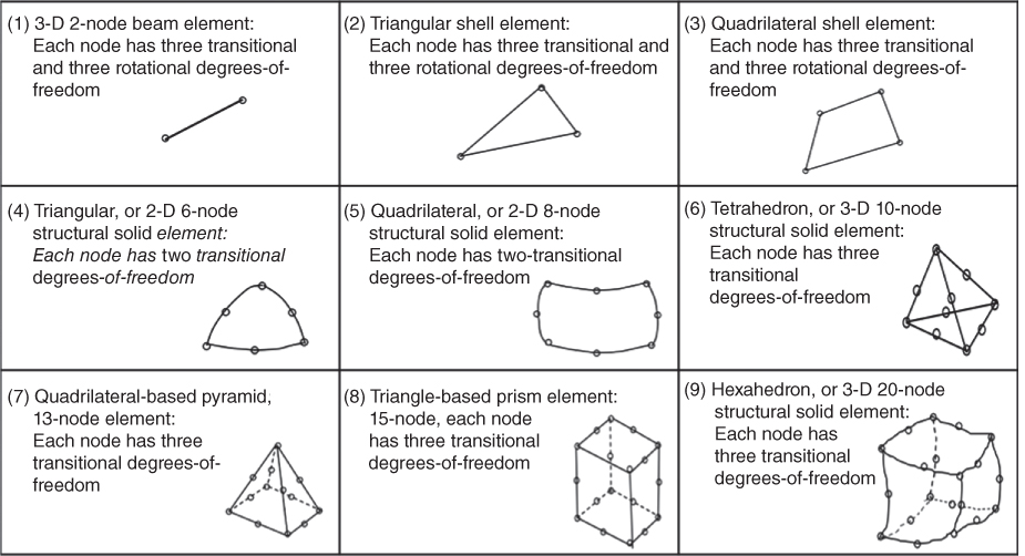
Figure 11.21 Advanced elements for finite-element models.

Figure 11.22 Finite-element analysis on imported solid geometry. (a) Imported solid geometry. (b) Finite-element analytical results.
(Courtesy of ANSYS Inc. , Pittsburg, PA, USA).
11.6.2 Simulation using general-purpose finite-element codes
A relatively new application of general-purpose finite-element code is to simulate critical engineering processes, in particular those involved in new product development. Such simulations may result in significant cost saving for the development process, and also reduce the time to market for these products. While the process of product development may vary from case to case, Figure 11.23 illustrates the general procedure with various stages in such a development.

Figure 11.23 General processes in new product development.
A recent article on “What does product development really cost” by K. Douglass [http://www.pivotint.com] reports some resounding outcomes, such as that a 12-month in reduction in time-to-market (TTM) would result in 92% increase in “internal rate of return” (IRR) on the product development investment. A 63% increase in IRR was achieved with a 9-month reduction in TTM. Further observation indicates that other than the costs of personnel and management, and the market research activities, the most costly activities in new product development are the design, production, and testing of the two prototypes, as indicated in Figure 11.23. Not only are activities relating to the prototyping costly, they also prolong time-to-market.
General-purpose finite-element code such as ANSYS has developed such capability that it can simulate many of the activities involved in product development that are shown in Figure 11.23. It can produce high-quality simulation based on expected functions of products of complex geometry subjected to all conceivable loading conditions. It also provides graphic simulations of what “real” physical prototypes can achieve under all conceivable conditions and beyond, which results not only in substantial savings in costs of building the real prototypes but also in substantial time saving in production and testing of the product using the virtual prototypes.
Figure 11.24 illustrates a case of simulation by the ANSYS code of various vibrational modes of the disk-and-pad assembly of an automobile braking system. The design objective of this system was to identify the onset of instability in braking using a modal analysis. The ANSYS solution from simulating the performance of a new design of a braking system such as shown in Figure 11.24 enabled engineers to achieve a first-time virtual design of a cost-effective, quiet braking system for multiple platforms in far less time than would have been possible with conventional methods using physical prototyping and field testing.
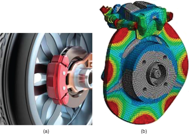
Figure 11.24 Simulation of the vibration of a disk-coupler during braking of a vehicle. (a) New design of braking pad. (b) Mode shape of disk.
(Courtesy of ANSYS Inc. , Pittsburg, PA, USA).
Problems
-
11.1 Use no more than 25 words in the answers to each of the following questions: (1) Why does the discretized FE model used in FEA lead to approximate but not the exact solutions to the real problems? (2) What is the major error induced in FEA with simplex elements using linear polynomial functions for the interpolation functions in the FEA? (3) How do you get more accurate results from the FEA involving simplex elements in question (2)? (4) What is the principal reason for using general-purpose FE codes to simulate new product development?
-
11.2 Show that the nodal force vector in stress analysis of an element may be expressed as
in which matrix [B(r)] is given in Equation 11.39 with r being the coordinates, {σ} is the stresses in the element, and v is the volume of the element.
-
11.3 Derive the interpolation function for a triangular toroidal element as illustrated in Figure 11.2. The cross-section of the element is made of nodes i, j, and k located at (ri,zi), (rj, zj), and (rk,zk), respectively, in the r–z coordinate system, with the z-coordinate being the axis of symmetry. Assume that the element displacement components in the radial and axial directions obey linear polynomial functions
 , and
, and  in which b1, b2, b3, …, b6 are arbitrary constants.
 -
11.4 Find the total elongation and the displacement at the nodes that join the three different rods in a compound bar as illustrated in Figure 11.25. The structure is similar to that in Example 11.5 but now with a third rod made of steel with Young's modulus
 .
.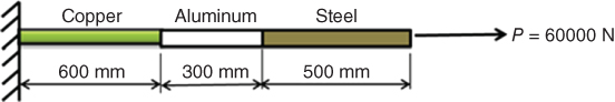
Figure 11.25 A compound bar made of three different materials.
-
11.5 Solve Problem 11.4 with the rods of copper and steel swapped in their respective positions in the compound bar in Figure 11.25. Compare the results in elongations of the three rods with those computed by formulae given in books of classical mechanics of materials.
-
11.6 Use the finite-element technique with a linear polynomial function for the interpolation function to compute the stresses and strains in the triangular plate element in Figure 11.26. Also find the displacement at the three nodes. The plate element is subjected to a force acting at node B. Use the material properties
 GPa and
  in your computations. The thickness of the plate element is 20 mm.
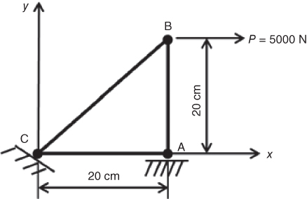
Figure 11.26 A triangular plate subjected to a nodal force.
-
11.7 Solve the displacements, strains, and stresses in a triangular plate similar to that in Problem 11.6 but with the applied force at node B with an angle of 30° downward from the x-axis.
-
11.8 Use the finite-element method to compute the following quantities for the triangular plate in Figure 11.27:
- a. Displacement components at the corners in the x- and y-directions.
- b. The stresses and strains in the plate.
- c. Reactions at the supports at nodes A and C.
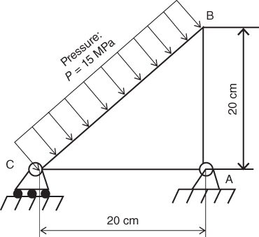
Figure 11.27 A triangular plate subjected to uniform pressure loading.
11.8 The plate is made of aluminum alloy with Young's modulus E = 70 GPa and Poisson's ratio
 .
.11.8 Hint: The distributed pressure loading on the edge of an element of the finite-element model may be treated as concentrated forces equally acting on the two adjacent nodes of the edge over the plane area of the edge. The plate is 20 mm thick.
-
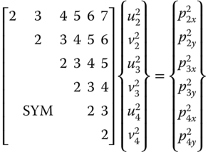
11.9 Show the overall finite-element equation similar to Equation 11.45 for a plane structure defined by an x–y coordinate system as an assembly of two elements with the individual element equations being as follows:
11.9 For Element no. 1:
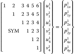
and for Element no. 2:
-
11.10 Use the finite-element method to solve the same problem as in Problem 11.6 with two elements in the discretized model as illustrated in Figure 11.28. The finite-element model in Figure 11.28 involves an additional node (node D) situated half-way between nodes B and C, and the numbers in circles are the element numbers in the model. Show what lesson you have learned from solving Problems 11.6 and 11.10.

Figure 11.28 Finite-element model of a triangular plate with two elements.