Appendix 4
Application of MATLAB Software for Numerical Solutions in Engineering Analysis
Contributed by Vaibhav Tank
As described in Section 10.6.2, the MATLAB software package offered by The MathWorks, Inc. provides a powerful environment for numerical computations, visualization, and programming for engineers in their engineering analyses. Engineers may use this software package to quickly solve complex mathematical problems, analyze data, and develop algorithms, which would otherwise be extremely tedious to solve using traditional methods. This appendix will present three case examples to illustrate how MATLAB can be used to solve different types of problems in engineering analysis with a detailed description of the input/output procedures for using this software package. These selected cases are related to the examples in various chapters of the book.
The author of this book and the contributor of this appendix would like to express their appreciation to The San Jose State University for providing them the access to a late version of MATLAB R2015a used to solve the following three cases:
Case 1: Plot the instantaneous amplitudes of a vibrating mass y(t) in Equation 8.40 in Chapter 8, where t is the time after the inception of the vibration in a near-resonant vibration situation illustrated in Figure 8.24.
The solution of the instantaneous amplitudes of the vibrating mass M subjected to a cyclic force with circular excitation frequency ω is expressed as:

where ![]() is the maximum value of a cyclic force F0cos(ωt) applied to the elastic bench support of a stamping machine in Figure 8.19 with the mass
is the maximum value of a cyclic force F0cos(ωt) applied to the elastic bench support of a stamping machine in Figure 8.19 with the mass ![]() and the natural frequency of the vibrating bench
and the natural frequency of the vibrating bench ![]() . The frequency ω of the excitation force is 4.95 rad/s.
. The frequency ω of the excitation force is 4.95 rad/s.
The process of plotting the required graphic solution in Equation 8.40 with assigned numerical data using the MATLAB software package begins with the following steps:
- 1. Open the version of MATLAB installed in the computer.
- 2. Go to File – New – Script (Ctrl + N or
 + N) to create a new script file that MATLAB will run.
 - 3.
By looking at the problem statement, we can see that we have all of the variables needed to obtain the graphic solution of Equation 8.40. The only variable in this equation is t (time), so we will list it as such in the beginning. As with any mathematics or physics problem, we will start the solution procedure by listing all available information as:
syms t;         %Define system variables
Fo=1000;        %Excitation force in N
M=1000;         %Mass in kg
omega_o=5;      %Natural frequency of system in rad/s
omega=4.95;     %Excitation frequency in rad/s
The statements followed by the percentage symbol (%) are in-line comments. The compiler ignores everything following the symbol on that line. Comments are a great way to keep the user's thoughts organized, so that anyone who might look at the code later can understand what the user was thinking. MATLAB does not require the user to end each statement with a semicolon. In MATLAB, semicolons are used to construct arrays and separate commands on the same line, or to suppress the outputs. In this case, we used the semicolon at the end of each line for latter function, or else the result of that command would return to us through the Command Window. We will observe this later on in the code when we will purposely leave out the semicolon, so that we can actually obtain the result of that line of code.
We note that the value of epsilon (ϵ) is not explicitly expressed in Equation 8.40. This quantity is given by the following expression in this book:
8.39b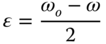
Converting the above relation into the MATLAB code, we get the following:
epsilon=(omega_o‐omega)/2;     %Circular frequency (epsilon)
                               %calculated from natural and
                               %excitation frequency
We also need to define the “vector” for the variable t with a specified step size.
t=[0:.01:10]; % array for time valuesHere, the vector t starts at 0 and continues up to 10 seconds with a selected step size of 0.01 seconds. There is a reason for choosing such a small step size, as will be discussed later. Now that we have all of the required variables defined, we can go ahead and specify the solution of the equation that needs to be plotted graphically. One important thing to keep in mind is that most of the variables we defined so far are scalars, but the array t is treated as a vector. In order to multiply scalars and vectors together, MATLAB uses special notations to signify element-wise multiplication, where one may use a period (.) in front of the operator as shown below:
y=(2.*Fo)./(M.*(omega_o<sup>∧</sup><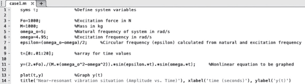
- 4. Click on the green “play” icon in the ribbon on the computer screen to run the script.
Output:
We note that two different trigonometric functions are present in Equation 8.40 along with the coefficient in the square brackets. Both these trigonometric functions and the associated coefficient play important roles in the output results. The quantity in the square brackets represents the maximum oscillating amplitude of the vibrating mass. The function sin(ϵt) regulates the variation of the amplitudes in shorter periods as seen in Figure A4.1. However, in order to see how sin(ωt) plays a role in this near-resonant vibration situation, we need to zoom out the graphing window and edit line 9 in the script:

Figure A4.1 Amplitude of the vibrating mass in the first 20 seconds.
t=[0:.01:125]; % array for time valuesWe would then run the script again resulting in the following graph:
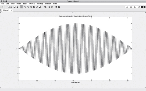
Increasing the value of t to 250 seconds by editing the same line, one can see the behavior of the entire function.
From this graph, we can see that the effect of the second sinusoidal function sin(ωt) produces fluctuation of the variations of the amplitudes produced by the function sin(ϵt) in a wave-like behavior as shown in Figure A4.3.
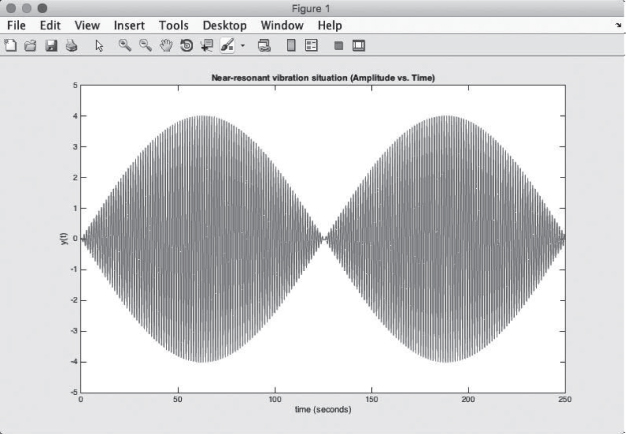
Figure A4.3 Amplitude of the vibrating mass after one complete cycle.
While preparing the input to the MATLAB code in this particular case, we made a decision on purposely using a small step size in order to capture every “small cycle” of the vibrating mass (call “beats”) in the graphic display. Not having the appropriate step size, also called undersampling, can result in aliasing, which creates a distorted view of the actual results. If we had chosen a step size of t = 5 s instead of 0.01, the results would have been as shown in Figure A4.4.

Figure A4.4 Improper graphical results due to aliasing.
The user is thus reminded that undersampling, in this particular case illustration, could lead to improper results that do not resemble those shown in Figures A4.1-A4.3, because we are capturing data points that are too large of an interval than the true behavior of the solution of Equation 8.40. Thus, it is important to choose the correct solution step sizes to ensure that we get the correct representation of the function y(t).
Case 2: On the mode shapes of a vibrating flexible pad
This case deals with the determination of the shapes of Mode 1 and of a vibrating flexible pad from a free vibration analysis. Flexible pads are reasonable approximation of thin plate structures.
We will use the MATLAB software package to generate graphical solution to the free vibration analysis of a flexible pad described in Section 9.8 with the following physical conditions:
The pad has a rectangular shape as illustrated in Figure 9.25 with length b = 10 inches and width c = 5 inches. The pad has a thickness of 0.185 inch and a mass density of 1.55 lbm/in2. The pad has an initial sag due to its own weight, which can be described by a function ![]() , and this shape is sustained by a tensile force
, and this shape is sustained by a tensile force ![]() .
.
We performed the following procedures for deriving the required graphical solutions by using the MATLAB software package:
- 1. Open the version of MATLAB in the computer.
- 2. Go to File – New – Script (Ctrl + N or + N) to create a new script file that MATLAB will run.
- 3. Since the solution of free vibration of flexible pads is already available as Equation (9.76) in the book, with the induced amplitudes of the vibrating pad expressed in Equation 9.81, we will focus on creating surface plots using the latter equation.
- 4. We will put an effort to list all the given variables as shown below:
syms x y % Define variables to be graphed b = 10; % Length of pad in inches c = 5; % Width of pad in inches P = 0.5; % Tension applied to pad in lb<sub>f</sub><
and the constant coefficient a in Section 9.8.3 to be:

Using the above equations, we can let the MATLAB to perform the calculations with the following lines of code:
w_mn = sqrt((m*pi/b)<sup>∧</sup><![CDATA[2+(n*pi/c)<sup>∧</sup><![CDATA[2);      % Frequency in rad/s
a = sqrt(P*g*12/ρ);                % Constant coefficient in
in/s; formula multiplied by 12 to convert from feet to inches
In order to calculate the required mode shapes of the flexible plate, we also need to determine the coefficient Amn using the following equation:
where b = 10 inches and c = 5 inches. The input for evaluating the coefficients Amn to the MATLAB code is:
A_mn = (16*(b*c)<sup>∧</sup><![CDATA[2*(1+(-1)<sup>∧</sup><![CDATA[(n+1))*(1+(-1)<sup>∧</sup><![CDATA[(m+1)))/(m<sup>∧</sup><![CDATA[3*n<sup>∧</sup><![CDATA[3*pi<sup>∧</sup><![CDATA[6);
% Calculate coefficient A_mn
One reason to use MATLAB scripts is that they make computing tedious and repetitive calculations easy and quick with just a few lines of code. We will create a while loop in MATLAB to iterate through different time intervals at which we would like to compute the equation. To begin the loop, we have to initialize the iterating variable T as follows:
T = 0;     % Initialize time in seconds
f = 1;     % Initialize figure label counter
After initializing the variables, we have to define the boundary conditions at which we would like to end the loop. In this case, we want to run the loop up to time t = 0.25 seconds, which should give us a good view on the shapes of the pad immediately after it is subjected to an instantaneous disturbance. The corresponding input coding is:
while T <= 1/4    % While loop to create graphs at different time
intervals
The goal of this “while loop” is to create multiple surface plots at different time intervals. Thus, it is important to create figure labels with the figure( ) command, as shown below:
figure(f) % Figure labelAlthough this may not seem like a crucial command, not including this one line in the script will overwrite the previous plot as soon as each loop has been executed. Thus, leaving out the figure( ) command will produce only one graph instead of three, as we intended.
Now that all the variables are accounted for in the input file, we need to define the equation whose results need to be displayed graphically:
where x and y are the coordinates for the length and width of the pad, respectively.
      z = A_mn * sin(m*pi*x/10) * sin(n*pi*y/5) * A_mn *
(cos(a*w_mn*(T)));     % Function to be graphed
In order to create the contoured surface plots, we will use the built-in ezsurfc( ) function to perform this task. The input parameters include the function that needs to be displayed graphically, followed by the domain in vector format. The first two parameters in the array correspond to the x domain and the last two parameters correspond to the y domain.
  ezsurfc(z,[0, 10, 0, 5]) % Function to create a contoured surface
graph
To assign the appropriate plot titles, we will use the built-in string concatenation function strcat() to create the correct string str that will be used in the titles for each plot. This function concatenates strings horizontally separated by commas as shown below:
  str = strcat('Shape of the pad at ', 'T = ', num2str(T), '
seconds', ' in Mode ', num2str(m)); % Concatenate strings for figure
title
    title(str)
An important thing to keep in mind is that the function takes only the arguments of type string, which is why we had to convert the variables T and m to strings using num2str(). Otherwise, MATLAB will throw an error that reads “Inputs must be cell arrays or strings.”
The main part of the loop is now over. However, in this “while loop,” we need to specify how to increment the iterating variable T as well as f, which is used in the figure labels. Without specifying the increments of T, MATLAB will not know how to proceed, which will create an infinite loop and eventually crash the application. At the end of the “while loop,” we need to let MATLAB know that we have reached its terminating point by using the end command. Thus, the following lines of code are very important:
    T = T + 1/8; % Increment time by 1/8 seconds.
    f = f + 1;   % Increment figure number
end
The input file to MATLAB in this case is now completed, and we are ready to run the case by the MATLAB code. The following is the input data file for the user to make a final check for its appropriateness.

4.5 Click on the green “play” icon on the computer screen to run the case after having been ensured with the correct inputs to the problem.
Output:Mode 1:
Figures A4.5a,b,c show the shape of the pad in Mode 1 at different times. Although the shapes look similar to each other, one can observe the reduction in the maximum amplitude by looking at the changes in the scale of the amplitude on the left. There is a drastic drop in the amplitude between t = 0 s and t = 1/4 s, as shown in Figures 4.5a and 4.5c. In order to see what happens to the pad under Mode 3 vibration, we need to go back to the input file again and change m and n to 3 in lines 8 and 9, respectively.
m = 3;     % Mode variable
n = 3;     % Mode variable
Figure A4.5a Initial shape at t = 0 s of the flexible pad.

Figure A4.5b Mode shape at t = 1/8 s.
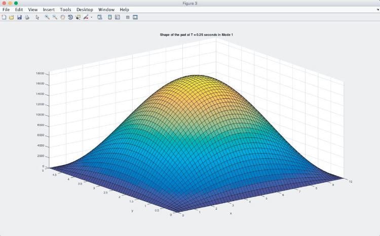
Figure A4.5c Mode shape at t = 1/4 s.
After pressing the “play” button again, we get the following results:
Mode 3:
Figures A4.6a,b,c show the shape of the flexible pad in Mode 3 vibration. Multiple peaks are present in this mode, both along the x- and y-directions. The figure above overlays a contour plot on a surface plot in order to show the locations where the peak amplitudes occur. These locations are of particular interest to engineers during vibrational analysis and the results were achieved by using the ezsurfc( ) function of MATLAB.
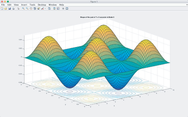
Figure A4.6a Initial state of the pad (t = 0 s).
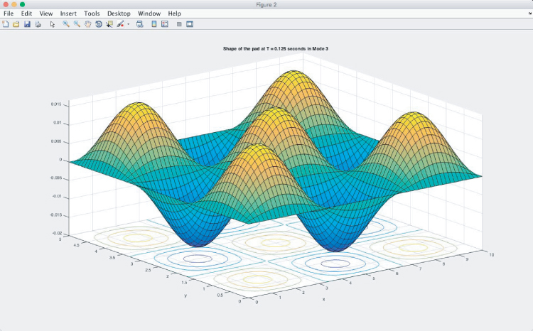
Figure A4.6b Mode shape at t = 1/8 s.
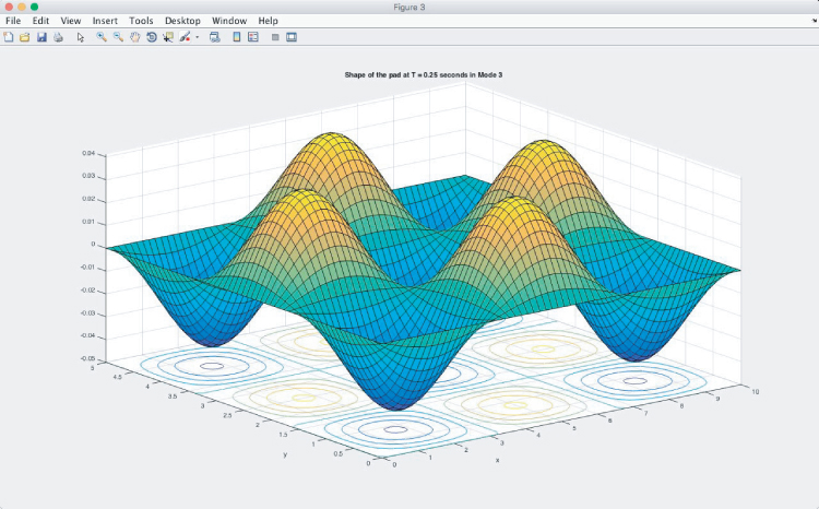
Figure A4.6c Mode shape at t = 1/4 s.
Case 3: Solve the following ordinary differential equation with graphic output (Example 10.15 in the book):

with y(0) = 0 and y'(0) = 0
The reader will find from Example 10.15 in Chapter 10 that a fourth-order Runge–Kutta method was used to solve the ordinary differential equation, Equation (a), but not without lengthy computations of several recurrence relations provided by this method. Here, the reader will find that solution with significant easiness is obtainable by using the MATLAB software package, with the additional capability of the graphic output for the solution. The procedure for obtaining the MATLAB solution of this differential equation is as follows:
- 1. Open the version of MATLAB in the computer.
- 2. Go to File – New – Script (Ctrl + N or + N) to create a new input (script) file that MATLAB will run.
- 3.
To begin solving this problem, we will need to create two functions: one that defines the second-order ordinary differential equations (ODEs) in terms that are acceptable by MATLAB, and the second one that solves the equation using a built-in solver.
We can name the function the way we like; the only restriction is that the filename should match the exact name of the function. This script uses a main function that calls the definition of the differential equation. However, the user is free to create separate scripts for each of the functions. We will define an arbitrary range of x-values and list the given initial conditions for this equation as:
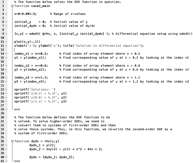
function case2_main
x=0:0.001:3;          % Range of x-values
initial_y    = 0;     % Initial value of y
initial_dydx = 0;     % Initial value of dy/dx
There are several built-in “ordinary differential equation” solvers within MATLAB, but ode45( ) is one of the most versatile and should be the first solver that one should try to solve most problems. For instance, on the left-hand side of Equation (a), one should state the two variables involved in the equation using a vector. The ode45( ) function on the right-hand side takes in the parameters such as the function, the range of values, and the initial conditions. One thing to keep in mind is that this solver is capable of solving only the first-order ordinary differential equations (ODEs), so derivatives in the higher-order equations need to use a special command, as will be seen a little later.
[x,y] = ode45( @rhs, x, [initial_y initial_dydx] ); % Differential
equation setup using ode45()
Now that we have the equation defined, the only thing left to do is plotting the results; the solver takes care of the rest. Because of the initial conditions defined in the ode45( ) solver, the y-vector returns two columns: y(t) and dy/dt. When creating the plot, we only want to plot the first column of the y vector against the x-axis since that is the solution to the problem. When referencing a matrix in MATLAB, one needs to reference it using the following format: matrix_name(row, column). Because we want to plot graphs for all of the rows of the first column of the y matrix, we use y(:,1) as shown below.
plot(x,y(:,1));
xlabel('t'); ylabel('x'); title('Solution to differential equation');
At this point, the main function is complete. The lines of code below are used to confirm the solutions with that of Example 10.15 in the book which was solved using the fourth-order Runge–Kutta method. We would like to confirm the y-values at specific x-values. In order to do this, we need to find the index of a specific x value first by searching through the x matrix. The next few lines of code search through the x matrix with x = 0.2, 0.6, and 1.2, respectively. These index values are stored in their corresponding variable names and are then used to search through the y matrix to find the exact value of the solution at the index as:
index_x1 = x==0.2;  % Find index of array element where x = 0.2
y1 = y(index_x1);  % Find corresponding value of y at x = 0.2 by
looking at the index x1
index_x2 = x==0.6;  % Find index of array element where x = 0.6
y2 = y(index_x2);  % Find corresponding value of y at x = 0.6 by
looking at the index x2
index_x3 = x==1.2; % Find index of array element where x = 1.2 y3 = y(index_x3); % Find corresponding value of y at x = 1.2 by looking at the index x3After storing the exact values found by searching through the arrays, we can print the results on the Command Window by using the sprintf( ) commands. Strings used within this command are enclosed within quotation marks. The user may also use formatting operators as placeholders for variables within a print statement. In this case, we use the %f formatting operator because we know that the results from the ode45( ) solver will contain float values. The decimal value (.3) in front of the format specifier indicates the number of decimal places the user wants to print. We chose to print three decimal places to avoid too much clutter. As shown below, the format specifiers are replaced with the variables that follow the commas.
sprintf('Solutions: ')
sprintf('y(0.2) = %.3f', y1)
sprintf('y(0.6) = %.3f', y2)
sprintf('y(1.2) = %.3f', y3)
end
So far, we have set up the parameters in the ode45( ) solver and plotted them, but the function needs to be defined yet. We start off by naming and creating a function called rhs containing the equation that needs to be solved; this will then be used in the ode45( ) solver. Earlier, we mentioned that the solvers can only solve first-order ODEs, so we need to be creative in converting the second-order ordinary differential equations (ODEs) that we want to solve into two first-order ODEs as follows:
We will express Equation (a) in the form of the first-order differential equation by redefining
 as a function y(2) and move all other terms in Equation (a) to the right-hand side of the equation as follows:
where the functions
 and
and  .
.The solution to this problem will be represented as a vector
 . Keep in mind that only y(1) corresponds to the solution of y in the original equation and the function y(2) corresponds to the derivative of y(x), which can just be ignored as a byproduct of this method. This is the reason why we seek only the graphical solution of the first column of the y-vector in the plot( ) function. Once this is done in defining the differential equation to the first-order ODE, we need to terminate it with the end command.
function dydx = rhs(x,y)
    dydx_1 = y(2);
    dydx_2 = 2*y(2) - y(1) + x<sup>∧</sup><![CDATA[2 - 4*x + 2;
    dydx = [dydx_1; dydx_2];
end
The above action marks the completion of the entire script. Double-check the cursor to make sure that the displayed script matches the one shown below:
- 4. Click on the green “play” icon appearing on the computer screen to run the case computation.
Output:
>> case2_main
ans =
Solutions:
ans =
y(0.2) = 0.040
ans =
y(0.6) = 0.360
ans =
y(1.2) = 1.440
>>
Figure A4.7 Solution to the second-order differential equation.