Chapter 10
Numerical Solution Methods for Engineering Analysis
10.1 Introduction
Numerical methods are techniques for solving the mathematical problems involved in engineering analysis that cannot be solved by closed-form solution methods such as those presented in the preceding chapters. In this chapter, we will learn the use of some of the available numerical methods that will not only enable engineers to solve many mathematical problems, but also allow engineers to minimize the need for the many hypotheses and idealization of the conditions, such as those stipulated in Section 1.4.
Numerical techniques have greatly expanded the types of problems that engineers can solve, as illustrated in a number of publications in the open literature (Chapra, 2012; Ferziger, 1998; Hoffman, 1992). The goal of this chapter is to present to readers the basic principles of some of these techniques that are frequently used in engineering analysis. The author's own experience indicates that engineers who understand the principles of the numerical methods are usually more effective and intelligent users of these methods than most technical personnel who are trained to carry out the same computational assignments using “turn-key” software packages such as the finite-difference method and the MatLAB software package in Appendix 4. This chapter will cover the principles of commonly used numerical techniques for (1) the solution of nonlinear polynomial and transcendental equations; (2) integration involving complex forms of functions; and (3) the solution of differential equations by the basic finite-difference schemes and the Runge–Kutta methods. The chapter will also cover the overviews of two popular commercial software packages called Mathematica and MatLAB.
The principal task in numerical methods for engineering analysis is to develop algorithms that involve arithmetic and logical operations so that such operations can be performed at incredible speed by digital computers with enormous data storage capacities. Because readers of this book are expected to be users of numerical methods, we will present only the principles that are relevant to the development of these algorithms, not the theories and the proof of these methods.
10.2 Engineering Analysis with Numerical Solutions
Most engineering problems require enormous computational effort when numerical methods are used. Digital computers are essential tools for obtaining numerical solutions. Digital computers have incredible power in computational speed and enormous memory capacity. Unfortunately, these machines have no intelligence of their own, and they are not capable of making independent judgment on their own. Additionally, engineers need to realize the fact that digital computers can only perform simple arithmetic operations with (+, −, ×, ÷) and handle the logical flow of data. It cannot perform higher mathematical operations even in such simple cases as evaluating exponential and trigonometric functions without proper algorithms that convert the evaluation of these functions into simple arithmetic operations; thus, all complicated mathematical operations have to be converted into simple arithmetical operations. Numerical methods that enable engineers to develop algorithms for various mathematical functions and operations using digital computers have thus become essential knowledge and skills for solving many advanced engineering problems using mathematical tools.
Despite the fact that numerical techniques have greatly expanded the types of problems that engineers can handle as mentioned in Section 10.1, users need to be aware of many unique characteristics of these methods, as outlined in the following.
- 1. Numerical solutions are available only at selected (discrete) solution points of the domain that is being investigated, not at all points in the entire domain covered by the functions as is the case with analytical solution methods described in Chapters 7, 8, and 9.
- 2. Numerical methods are essentially “trial-and-error” processes. Typically, users need to know the initial and boundary conditions that the intended solution will cover. The selection of increments of the variable at which the solution points are positioned is critical in the solution of the problem. Unstable numerical solutions may result from improper selection of such increments, called the step sizes with solutions.
- 3. Most numerical solution methods result in some error in the solutions. Two types of error are inherent with numerical solutions:
- a. Truncation errors – because of the approximate nature of numerical solutions of many engineering problems, these solutions often consist of both lower-order terms and higher-order terms. The latter terms are often dropped in the computations in order to achieve computational efficiency, resulting in error in the solution.
- b. Round-off errors –Most digital computers handle numbers either with 7 places or 14 decimal places in numerical solutions. In the case of a 32-bit computer with double precision (i.e., numbers of 14 decimal places), any number after the 14th decimal point will be dropped. This may not sound like a big deal, but if a huge number of operations are involved in the computation, such error can accumulate and result in significant error in the end results.
Both of these types of error are of cumulative nature. Consequently, errors in numerical solution may grow to be significant in solutions obtained after many step increments.
10.3 Solution of Nonlinear Equations
Often, engineers need to solve nonlinear equations in their analyses. These equations can be as simple as quadratic equations such as in Equation (8.3) with the two roots expressed in Equation 8.4. There is also the need to find roots of equations in higher-order polynomial functions such as shown in Equation 10.1, relating to the problem of locating the marking on a measuring cup, to be described in Example 10.3 and in Figure 10.4:
or solution of the time tf required for the mass to rupture from its spring attachment in the case of resonant vibration analysis that was illustrated in Example 8.9:

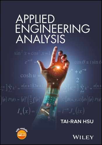
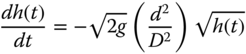
Solutions of nonlinear equations such as Equations 10.1 and 10.2 may be obtained by setting expressions f(x) = 0, and finding their roots (i.e., L in Equation 10.1 and tf in Equation 10.2) located at the points of cross-over of the function f(x) and the x-coordinate axis, as illustrated in Figure 10.1.

Figure 10.1 Root of a nonlinear equation  .
.
We will use the following two methods for the solution of the nonlinear equation given in Equation 10.2
10.3.1 Solution Using Microsoft Excel Software
Because the roots of an equation represented by f(x) = 0 are located at the intersections of the function f(x) and the x-coordinate axis as illustrated in Figure 10.1, one may use the widely available tool of spreadsheets (such as Microsoft Office Excel) to locate the roots of the equation by evaluating the function f(x) with for various values of the variable x. The range in which the roots of the equation f(x) = 0 lie can be identified as the values where f(x) change sign from positive to negative or vice versa, as illustrated for the range (xi−1–xi+1) in Figure 10.1. More accurate values of the roots may be found by repeating the computation of the function values with smaller increments of the variable x within that range. This method, though sounds tedious, involves straightforward evaluation of the function f(x) with an initially estimated value of xi by using the Excel software that has enormous computational speed to identify the range in which the roots are located, as will be illustrated by Example 10.1.
10.3.2 The Newton–Raphson Method
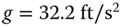
Perhaps the most widely used method for finding the roots of nonlinear equations is the Newton–Raphson method. This method offers rapid convergence to the roots of many nonlinear equations from the initially estimated roots. The fast convergence to true roots from the estimated roots is achieved by means of computation of both the function f(xi) and the corresponding slope f′(xi) of the function at xi, as illustrated in Figure 10.3.
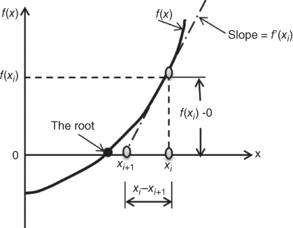
Figure 10.3 Newton–Raphson method for solving nonlinear equations.
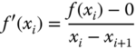
Figure 10.3 illustrates the principle of the Newton–Raphson method of solving nonlinear equations. As in many other numerical solution methods, the user has to estimate a root at x = xi for the equation f(x) = 0, from which they may compute the function f(xi) and at the same time the slope of the curve generated by the function f(x). This slope may be expressed f′(xi). The graphical representation of this situation indicates that the slope f′(xi) may be expressed by Equation 10.4:
which leads to the following expression for the next estimated root at x = xi+1:

One readily sees from Figure 10.3 that the computed approximate next root xi+1 is much closer to the real root (shown as a solid circle) than the previous estimated value at xi.
10.4 Numerical Integration Methods
Integration of functions over specific intervals of the variables that define the functions is a frequent requirement in engineering analysis. Some of the practical applications of integration are presented in Section 2.3 in Chapter 2. Exact evaluation of many definite integrals can be found in handbooks (Zwillinger, 2003) but many others with functions to be integrated are so complicated that analytical solutions for these integrals are not possible. Numerical methods are the only viable ways for such evaluations.
In this section, we will present three numerical integration methods: (1) the trapezoidal rule; (2) Simpson's one-third rule; and (3) Gaussian quadrature. The first two methods are commonly used for integration of nonlinear functions, and the third method is extensively used in numerical analysis of complex engineering analyses, such as the finite-element analysis.
We will focus our effort on refreshing the principles that are relevant to the development of algorithms of these particular numerical integration methods, but will not rehearse the underlying theories and their proofs. The reader will find derivation of the formulae for these numerical integration methods in reference books such as those by Chapra (2012), Ferziger (1998), and Hoffman (1992).
10.4.1 The Trapezoidal Rule for Numerical Integration
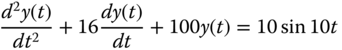
We learned in Section 2.2.6 that the value of a definite integral of a function y(x) is equal to the area under the curve produced by this function between the upper and lower limits of the integration as illustrated in Figure 10.6. Mathematically, the integral of function y(x) can be expressed as
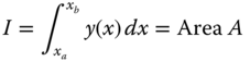

Figure 10.6 Graphical representation of integration of a continuous function.
The value of the integral of a function may thus be determined by computing the area covered by the function between the two specified limits. For example, the value of the function y(x) in Figure 10.7 may be approximated by the sum of the three trapezoidal plane areas A1, A2, and A3.
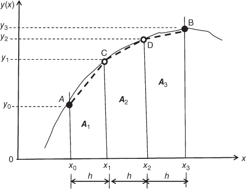
Figure 10.7 Approximation of the integral of a continuous function y(x).
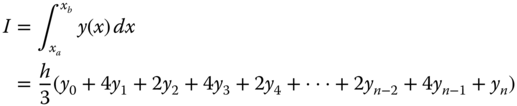
The area of a trapezoidal plane may be evaluated by the formula of half of the sum of the length of two parallel sides multiplied by the distance between these two sides. Mathematically, the plane areas A1, A2, and A3 with equal distance h between two parallel sides in Figure 10.7 may be computed by the following formulae:

The sum of A1, A2,and A3 is given by

in which h is the assigned increment of variable x, and y0, y1, y2, and y3 are the values of the function evaluated at x0, x1, x2, and x3, respectively.
This approximate value of the integral I obtained by the above formula is less than the analytical solution of 191.45 obtained from a mathematical handbook (Zwillinger, 2003). The difference between the value of the integral of 180.92 obtained using the trapezoidal rule and that of 191.45 from the analytical solution method is to be expected. This difference in results represents the errors inherent in any numerical method. In the trapezoidal rule method in this example, the discrepancy is introduced by the approximation of the curve representing the given function by straight line segments (shown dashed) that were the edges of the trapezoids in computing the approximate area under the curve in Figure 10.8. One may readily observe that this discrepancy between the curved edges and the straight edges shown as dashed lines can be reduced by the reduction of the size of the increment h, as can be observed from the graphic illustration in Figure 10.8. Consequently, closer approximation, or more accurate results from numerical integration, may be achieved by reducing the size of increment h in this particular numerical analysis.
Figure 10.9 shows the area under function y(x), which can be approximated as the sum of the areas of (n − 1) trapezoids. Many more trapezoids under the function curve such as shown in Figure 10.9 entails many more increments of h along the x-coordinate between the upper and lower integration limits, with concomitant more accurate results.
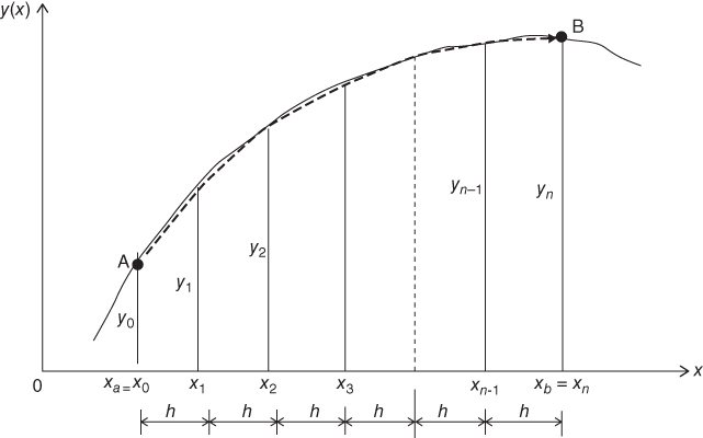
Figure 10.9 Integration of function y(x) with multiple trapezoids.
The approximate value of the integral of function y(x) in Figure 10.9 is equal to the sum of all the trapezoids in the figure according to the following equation derived from the same principle as in the earlier case with three trapezoids:

where h is the increment along the x-coordinate axis in the numerical integration.
This value of 188.88 for the same integral now with h = 0.5 is much closer to the analytical value of 191.45 than that of 180 obtained with h = 1.0 in Example 10.5. It has thus been demonstrated the fact that the smaller the increment one uses in numerical integration, the more accurate a result will be obtained.
10.4.2 Numerical Integration by Simpson's One-third Rule
In Section 10.4.1, we refreshed the principle of evaluating an integral as the plane area under the curve representing the function (the integrand) in the integral between two limits of the variable in the integration. This area is graphically expressed in Figure 10.11a.
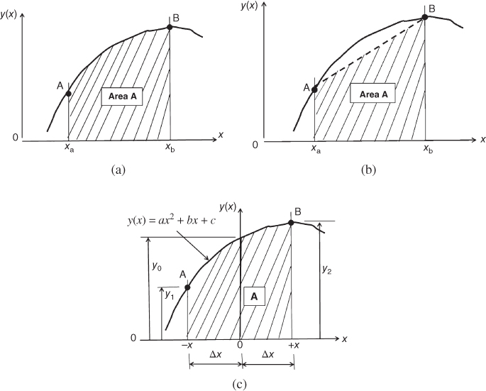
Figure 10.11 Graphical representation of integration of a continuous function. (a) Area defined by a function. (b) Approximation of the area by a trapezoid. (c) Approximation of the area by a parabolic function.
The value of an integral may be obtained by numerical methods such as the trapezoidal rule described in Section 10.4.1. The trapezoidal method is a simple but a relatively “crude” method that will result in an approximate value of the integral with minimal computational effort. Graphical representation of the trapezoidal method is illustrated in Figure 10.11b for the simplest possible numerical approximation of the area under the curve of y(x) as the area of one trapezoid (shown as the cross-hatched area) under the curve. This method is popular and easy to use because the formula used to compute the plane area of trapezoids is well known to engineers.
Another popular numerical method for integration is by Simpson's rule, in particular, “Simpson's one-third rule.” This rule differs from the trapezoidal method by assuming that the function y(x) can be approximated in the range of interest by a parabolic function as shown in Figure 10.11c. The function y(x) = ax2 + bx + c that describes the sector of the function in Figure 10.11c contains the unknown constant coefficients a, b, and c which can be determined with the following simultaneous equations relating to the function values at the discrete variable values x = −x , x = 0, and x = +x as follows:

from which we may solve for
The value of the integral of the function y(x) is equal to the plane area A in Figure 10.11c, or

By substituting the constant coefficients a and c in Equations 10.9a and 10.9b, together with Δx = x illustrated in Figure 10.11c, into the above expression, we get the following relation for Simpson's one-third rule for the integral I:
The analytical or “exact” result of the above integral is 191.45 from a table of definite integrals (Zwillinger 2003), which we may compare with the results I = 188.88 using three trapezoids in Example 10.5 and I = 194.70 with three function values using Simpson's one-third rule.
We will use the same illustration in Figure 10.13 and Equation 10.10 to derive the general expression for Simpson's one-third rule for numerical integration.

Figure 10.13 Integration of a nonlinear function y(x) by Simpson's one-third rule.
We derived Equation 10.10 with the first three function values y0, y1 and y2 at x = x0, x = x1, and x = x2, respectively, with an assumed parabolic function connecting these three points. The next parabolic function for the next adjoining three-point segment requires that the function value y2 be evaluated twice. The same happens to the second last point at xn−1 in the region for the integration at which the function value yn−1 in Figure 10.13 being evaluated twice. The coefficients associated with the yi for n points in Figure 10.13 are given in the following tabulation:
| xi | 0 | 1 | 2 | 3 | 4 | 5 | 6 | … | n−2 | n−1 | n |
| Coefficient of yi | 1 | 4 | 2 | 4 | 2 | 4 | 2 | … | 2 | 4 | 1 |
We may thus formulate the general expression of Simpson's one-third rule as follows:
We note from Equation 10.11 that the use of this relationship for Simpson's one-third rule requires even number of function values with odd number increments in the integration variable.
10.4.3 Numerical Integration by Gaussian Quadrature
Numerical integration of functions using the trapezoidal rule (Section 10.4.1) and Simpson's one-third rule (Section 10.4.2) enables us to determine approximate values of integrals of continuous functions f(x) over a range of (xb–xa) into equal parts with increment of the variable Δx (or h) as shown in Figures 10.7 and 10.9. This process allows us to select the sampling points and evaluate the integral in terms of the discrete values of the function at these points. These methods usually work well with well-behaved functions in integrals such as the ones used in Examples 10.5 to 10.8. However, neither the trapezoidal rule nor Simpson's one-third rule offers any guidance on the selection of the size of the increment of the variable in these numerical integration methods. There are times when engineers are expected to find numerical values of integrals involving functions that have drastic changes of shape over the range of the required integration. The two methods already discussed do not yield good approximations of the numerical values of these integrals because of improper selection of sampling points. Thus, it is desirable to have a numerical integration method that offers criteria for optimal sampling points in numerical integration.
The Gaussian integration method was established on the basis of strategically selected sampling points. The normal form of a Gaussian integral can be expressed as

in which n is the total number of sampling points, and Hi are the weighting coefficients corresponding to sampling points located at ![]() as given in Table 10.3.
as given in Table 10.3.
Table 10.3 Weight coefficients of the Gaussian quadrature formula in Equation 10.12 (Kreyszig, 2011; Zwillinger, 2003)
| n | ±ai | Hi |
| 2 | a1 = 0.577 35 | H1 = 1.000 00 |
| a2 = −0.577 35 | H2 = 1.000 00 | |
| 3 | a1 = 0.0 | H1 = 0.888 88 |
| a2 = 0.774 59 | H2 = 0.555 55 | |
| a3 = −0.774 59 | H3 = 0.555 55 | |
| 4 | a1 = 0.339 98 | H1 = 0.652 14 |
| a2 = −0.339 98 | H2 = 0.652 14 | |
| a3 = 0.861 13 | H3 = 0.347 85 | |
| a4 = −0.861 13 | H4 = 0.347 85 | |
| 5 | a1 = 0.0 | H1 = 0.568 88 |
| a2 = 0.538 46 | H2 = 0.478 62 | |
| a3 = −0.538 46 | H3 = 0.478 62 | |
| a4 = 0.906 17 | H4 = 0.236 92 | |
| a5 = −0.906 17 | H5 = 0.236 92 | |
| 6 | a1 = 0.238 61 | H1 = 0.467 91 |
| a2 = −0.238 61 | H2 = 0.467 91 | |
| a3 = 0.661 20 | H3 = 0.360 76 | |
| a4 = −0.661 20 | H4 = 0.360 76 | |
| a5 = 0.932 46 | H5 = 0.171 32 | |
| a6 = −0.932 46 | H6 = 0.171 32 | |
| 7 | a1 = 0.0 | H1 = 0.417 95 |
| a2 = 0.405 84 | H2 = 0.381 83 | |
| a3 = −0.405 84 | H3 = 0.381 83 | |
| a4 = 0.741 53 | H4 = 0.279 70 | |
| a5 = −0.741 53 | H5 = 0.279 70 | |
| a6 = 0.949 10 | H6 = 0.129 48 | |
| a7 = −0.949 10 | H7 = 0.129 48 | |
| 8 | a1 = 0.183 43 | H1 = 0.362 68 |
| a2 = −0.183 43 | H2 = 0.362 68 | |
| a3 = 0.525 53 | H3 = 0.313 70 | |
| a4 = −0.525 53 | H4 = 0.313 70 | |
| a5 =0.796 66 | H5 = 0.222 38 | |
| a6 = −0.796 66 | H6 = 0.222 38 | |
| a7 = 0.960 28 | H7 = 0.101 22 | |
| a8 =− 0.960 28 | H8 = 0.101 22 |
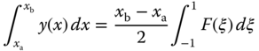
The form of Gaussian integral shown in Equation 10.12 is rarely seen in practice. A transformation of coordinate is required to convert the general form of integration such as shown in Equation 10.6 to the form shown in Equation 10.12, as illustrated in Figure 10.15.

Figure 10.15 Transformation of coordinates for Gaussian integration. (a) With the original coordinates. (b) After transformation of coordinates.
The transformation of coordinates from y(x) in the x-coordinate to the function F(ξ) in the coordinate ξ may be accomplished using the relationship
which leads to the following expression:
with
and
We will obtain the expression for the required evaluation of the integral in Equation 10.6 using Gaussian quadrature by substituting the relationship in Equation 10.12 into Equation 10.14.
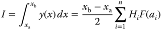
Numerical values of the weight coefficients Hi with sampling points ai are given in Table 10.3.
One needs to realize that the term F(ai) on the right-hand-side of Equation 10.15 denotes the function y(x) evaluated at the sampling points ai after it has been transformed to the function F(ξ) with integration limits of (−1 to +1) as in Figure 10.15b.
10.5 Numerical Methods for Solving Differential Equations
Differential equations frequently appear in engineering analysis, as described in Section 2.5. Many differential equations that engineers use for their analyses are “linear equations,” such as those presented in Chapters 7, 8, and 9, which can be solved by classical solution methods. There are, however, occasions in which engineers need to solve either highly complicated linear differential equations or nonlinear differential equations; in such cases numerical solution methods become viable alternative methods for finding solutions.
Numerical solution methods for differential equations relating to two types of engineering analysis problems: (1) “initial value” problems, and (2) “boundary value” problems. Solution of initial value problems involves a starting point with the variable of the function, say at x0, that is a specific value of variable x for solution y(x). With the solution given at this starting point, one may find the solutions at x = x0+h, x0+2h, x0+3h, …, x0+nh, where h is the selected “step size” in the numerical computations and n is an integer number of steps used in the analysis. The number of steps n in the computation can be as large as is required to cover the entire range of the variable in the analysis. Numerical solution to boundary value problems is more complicated; function values are often specified at a number of variable values, and the selected steps for solution values may be restricted by the specified values at these variable points.
There are numerous numerical solution methods available for the solutions of differential equations. It is not possible to cover all these solution methods in this section. What we will learn from this section is the principle of converting “differential equations” to “difference equations,” followed by numerical computation of solutions at discrete times or locations of the domain in the analysis. We will also confine our coverage to selected numerical solution methods involving only initial value problems. Readers are referred to reference books that have extensive coverage of numerical solutions for differential equations of both ordinary and partial differential equations, such as Ferziger (1998) and Chapra (2012).
10.5.1 The Principle of Finite Difference
We have learned in Chapter 2 that differential equations are equations that involve derivatives. Physically, a derivative represents the rate of change of a physical quantity represented by a function with respect to the change of its variable(s).
Referring to Figure 10.16, we have a continuous function f(x) that has values fi−1, fi, and fi+1 corresponding to the three values of its variable x at xi−1, xi, and xi+1, respectively. We may also write the three function values at the three x-values as
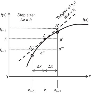
Figure 10.16 Function f(x) evaluated at three positions.
The derivative of the function f(x) at point A with x = xi in Figure 10.16 is graphically represented by the tangent line A″–A′ to the curve representing function f(x) at point A. Mathematically, we may express the derivative as given in Equation (2.9), or in the form
where Δx is the increment used to change the values of the variable x, and dx is the increments of variable x with infinitesimally small sizes.
One may observe from Equation 10.17 the important relation that the derivative may be approximated by finite increments of Δf and Δx as indicated in Equation 10.18:
if the condition on the increment Δx→0 is removed in the evaluation of the rate of change of the function f(x) in Equation 10.17.
Thus from Equation 10.17 we see that derivatives of functions may be approximated by adopting finite—but not infinitesimally small—increments of the variable x. A formulation with such an approximation is called “finite difference”.
10.5.2 The Three Basic Finite-difference Schemes
There are three basic schemes that one may use to approximate a derivative: (1) the “forward difference” scheme; (2) the “backward difference” scheme; and (3) the “central difference” scheme. Mathematical expressions of these difference schemes are given below.
- The forward difference scheme
In the “forward difference scheme,” the rate of change of the function f(x) with respect to the variable x is accounted for between the function value at the current value x = xi and the value of the same function at the next step, that is, xi+1 = x + Δx in the triangle ΔA′Aa′ in Figure 10.16. The mathematical expression of this scheme is given in Equation 10.19:
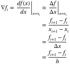
in which h = Δx is the “step size.”
The derivative of the function f(x) at other values of the variable x in the positive direction can be expressed following Equation 10.19 as

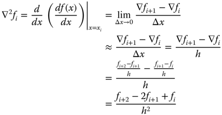
The second-order derivative of the function f(x) at x can be obtained according to the following procedure:
The backward difference scheme
In this difference scheme, the rate of the change of the function with respect to the variable x is accounted for between the current value at x = xi and the step backward, that is, xi−1 = x − Δx in the triangle ΔAA″a″ in Figure 10.16. The mathematical expression of this scheme is given in Equation 10.22:

Following a similar procedure as in the forward difference scheme, we may express the second-order derivative in the following form:

The central difference scheme:
The rate of change of function f(x) in this finite-difference scheme includes the function values between the preceding step at (x − Δx) and the step ahead, that is, (x + Δx). The triangle involved in this difference scheme is ΔA′A″a‴ in Figure 10.16. We have the first-order derivative as in Equation 10.24:
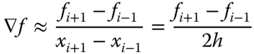
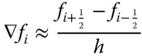
Note that in this finite-difference scheme a much larger step of size 2h is used in the first-order derivative as given in Equation 10.24. These “coarse” steps will compromise the accuracy of the values of the derivatives. A better central difference scheme is to employ for “half” steps in both directions. In other words, if we define
we will then have the derivative of the function f(x) using this modified central difference scheme as
One will observe from the tabulated values that the percentage error of the results obtained from the finite-difference method increases with the increase of the variable t. One may also show that the accuracy of the finite-difference method improves with smaller increments of the variables—the Δt in the present example.
10.5.3 Finite-difference Formulation for Partial Derivatives
Partial derivatives along a single dimension are computed in the same fashion as for ordinary derivatives (Chapra 2012) illustrated in Section 10.5.2. For example, the central difference scheme for function f(x,y) can be shown to have the following expressions:
The error of the above approximation is of order Δx = h.
For higher-order partial derivatives, such as ![]() :
:

Evaluating each of the partial derivatives in Equation 10.28 will lead to the following final expression:

The error of the approximation of second-order differentiation is of order (Δx)2.
10.5.4 Numerical Solution of Differential Equations
There are a number of numerical solution methods available for solving differential equations relating to both types of initial value and boundary value problems (Hoffman, 1992; Bronson, 1994; Ferziger, 1998; Chapra, 2012). We will present only the expressions used in the classic fourth-order Runge–Kutta method to illustrate the power of numerical methods for solving differential equations for initial value problems.
The simplest method of solving differential equations is to convert the derivatives in differential equations to the forms of “finite differences” as presented in Section 10.5.2 and Example 10.12. This method is straightforward but usually has significant accumulation of errors in the solution, as indicated in the numerical illustration in Example 10.12. There are several alternative versions available for solutions with better accuracies in the references cited above. We will include the Runge–Kutta method in this section for numerical solution of differential equations using initial value processes.
The Runge–Kutta methods are integrative methods for approximation of solutions of differential equations. These method, with several versions of the technique, were developed around 1900s by German mathematicians C. Runge and M.W. Kutta. The essence of the Runge–Kutta methods involves numerical integration of the function in a differential equation by using a trial step at mid-point of an interval—within a step Δx or h—using numerical integration techniques such as the trapezoidal or Simpson's rules as presented in Section 10.4. The numerical integrations will allow the cancellation of low-order error terms for more accurate solutions. Several versions of Runge–Kutta methods with different orders for solving differential equations have been developed over the years.
10.5.4.1 The Second-order Runge–Kutta Method
This is the simplest form of the Runge–Kutta method, with the formulation for the solution of first-order differential equation in the following form:
with a specified solution point corresponding to one specific condition for Equation 10.30. The solution points of this differential equation can be expressed as
where O(h3) is the order of error of the step h3, and
10.5.4.2 The Fourth-order Runge–Kutta Method
This is the most popular version of the Runge–Kutta method for solving differential equations in initial value problems. Formulation of this solution method is similar to that of the second-order method.
The differential equation is similar to that shown in Equation 10.30:
with the solution point given by the following formula:
where

10.5.4.3 Runge–Kutta Method for Higher-order Differential Equations
We have seen that Runge–Kutta method can solve differential equations often with remarkable accuracy as demonstrated in Example 10.14. Unfortunately, most textbooks offer the application of this valuable method only for solving first-order differential equations. Its use for solving higher- order differential equations requires the conversion of higher-order differential equations to the first-order-equivalent forms such as that shown in Equation 10.30. The solution of the converted higher-order differential equations can be obtained using expressions such as that given in Equation 10.33 for the fourth-order Runge–Kutta formulation. We will present the following formulation to illustrate how the fourth-order Runge–Kutta method can be used to solve second-order ordinary differential equations (the treatment is derived from an online tutorial http://www.eng.colostate.edu/∼thompson/Page/CourseMat/Tutorials/CompMethods/Rungekutta.pdf).
We will use the Runge–Kutta method to solve a second-order ordinary differential equation of the form

The left-hand side of Equation 10.35 may be expressed as dy′(x)/dx, which thus converts the second-order differential equation in (10.35) into a first-order differential equation in the form
with
Solution of the second order differential equation in Equation 10.35 may be obtained by the solutions of Equations 10.36a and 10.36b using the fourth-order Runge–Kutta formulations given in Equations 10.37 and Equation 10.38:
and
We note that the expression in Equation 10.38 is similar to that in Equation 10.33 for the converted first-order differential equation in Equation 10.36a.
The coefficients f1, f2, f3, and f4 in Equations 10.37 and 10.38 can be obtained from the expressions given in Table 10.4
Table 10.4 Coefficients in the fourth-order Runge–Kutta method for solving second-order differential equations
The three solution points at x = 0.2, 0.1, and 0.4 obtained by using the Runge–Kutta method appeared tedious and time-consuming. The same differential equation with the same specified conditions was solved using the software package MatLAB, with the input/output information included in Case 3 of Appendix 4. The results so obtained were remarkably accurate, with solution at the same three points being the exact values as shown tabulated above. MatLAB also offers graphical output such as that shown in Figure 10.17. An overview description of MatLAB software will be presented in Section 10.6.2.
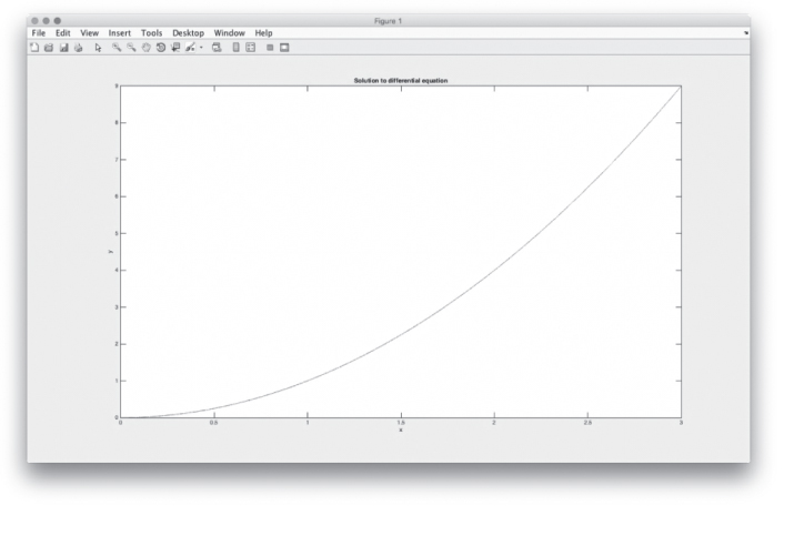
Figure 10.17 Graphical solution of a second-order ordinary differential equation by MatLAB.
This numerical solution has an error of 0.48% from the exact solution, and it is more accurate than that obtained from the simple forward difference scheme in Example 10.12.
10.6 Introduction to Numerical Analysis Software Packages
We have demonstrated the power, and thus the value of numerical methods in solving many problems in engineering analysis involving nonlinear equations, integrations, and differential equations in this chapter. These methods typically require significant time and efforts in arriving at approximate, not exact, solutions of the problem, and the solutions obtained are only available at discrete solution points. More accurate solutions are obtainable with small increment step sizes but with correspondingly more computational effort.
Since almost all the numerical methods involve massive computational effort and the solutions are available only at discrete solution points, sophisticated symbolic manipulation computer packages such as the popular commercially available Mathematica and MatLAB have proven to be valuable tools for engineers in engineering analyses associated with tedious computational processes. In this section, we will briefly survey these two numerical analysis packages, in particular their capabilities in solving engineering problems. Readers are referred to the literature for some excellent references (Malek-Madani, 1998; Chapra, 2012) providing more detailed descriptions and guidance on the effective use of these packages.
10.6.1 Introduction to Mathematica
Mathematica is a computational software program based on symbolic mathematics. It is used in many scientific, engineering, mathematical, and computing fields. The programming languages used in Mathematica are the Wolfram Language by Stephen Wolfram, together with C, C++, and Java. This software package has been in the marketplace since June 1988. It is capable of handling the following major functions and features in engineering analysis:
- 1. Determining roots of polynomial equations of cubic or higher orders.
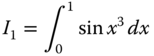
- 2. Integrating and differentiating complicated expressions. For instance, the integral of the function sin(x3), for which
 ; in contrast, similar integrals with the simple function sin(x) but with higher power of the function in the integral, such as
  , are available from integration tables in mathematical handbooks (Zwillinger, 2003).
 - 3. Solving linear and nonlinear differential equations.
- 4. Elementary and special mathematical function libraries.
- 5. Matrix and data manipulation tools.
- 6. Numeric and symbolic tools for discrete and continuous calculus.
It can also solve the following common analytical engineering problems:
- 1. Determining Laplace and Fourier transforms of functions.
- 2. Generating graphics in two and three dimensions.
- 3. Simplifying trigonometric and algebraic expressions.
According to the Wolfram Language and Systems Documentation Center, Mathematica has the following features and capabilities that are of great value in advanced engineering analyses:
- Support for complex number, arbitrary precision, interval arithmetic, and symbolic computation.
- Solvers for systems of equations, Diophantine equations, ODEs, PDEs, and so on.
- Multivariate statistics libraries including fitting, hypothesis testing, and probability and expectation calculations on over 140 distributions.
- Calculations and simulations on random processes and queues.
- Computational geometry in 2D, 3D, and higher dimensions.
- Finite-element analysis including 2D and 3D adaptive mesh generation.
- Constrained and unconstrained local and global optimization.
- Toolkit for adding user interfaces to calculations and applications.
- Tools for 2D and 3D image processing and morphological image processing including image recognition.
- Tools for visualizing and analyzing directed and undirected graphs.
- Tools for combinatorics problems.
- Data mining tools such as cluster analysis, sequence alignment, and pattern matching.
- Group theory and symbolic tensor functions.
- Libraries for signal processing including wavelet analysis on sounds, images, and data.
- Linear and nonlinear control systems libraries.
- Continuous and discrete integral transforms.
- Import and export filters for data, images, video, sound, CAD, GIS, documents, and biomedical formats.
- Database collection for mathematical, scientific, and socioeconomic information and access to Wolfram alpha data and computations.
- Technical word processing including formula editing and automated report generation.
- Tools for connecting to DLL, SQL, Java, .NET, C++, Fortran, CUDA, OpenCL, and http based systems.
- Tools for parallel programming.
- Mathematica language in notebook computers when connected to the Internet.
The last of the features listed is of particular value to engineers. For example, in Example 10.3 we were required to find the root of the cubic equation ![]() . A meaningful root of this equation found by the Newton–Raphson method was
. A meaningful root of this equation found by the Newton–Raphson method was ![]() as shown in Example 10.3. A similar solution of
as shown in Example 10.3. A similar solution of ![]() was obtained by the solution method offered via the internet at the Wolfram/Alpha Widgets website (www.wolframalpha.com/widgets/ ) with user input of the coefficients of this equation. It offered an instant solution and with an excellent user interface feature.
was obtained by the solution method offered via the internet at the Wolfram/Alpha Widgets website (www.wolframalpha.com/widgets/ ) with user input of the coefficients of this equation. It offered an instant solution and with an excellent user interface feature.
10.6.2 Introduction to MATLAB
MATLAB is an acronym of “matrix laboratory.” This numerical analysis package was designed by Cleve Moler in the late 1970s with an initial release to the public in 1984. The latest version, Version 8.6 was released in September 2015.
MATLAB provides a multiparadigm numerical computing environment and fourth-generation programming language, a proprietary programming language developed by MathWorks. It allows matrix manipulations, plotting of functions and data, implementation of algorithms, and creation of user interfaces that include interfacing with programs written in other languages, including C, C++, Java, Fortran, and Python. It is a popular numerical analysis package mainly because of it has graphics and graphical user interfacing programming capability.
Like Mathematica, MATLAB is capable of handling the following common problems in engineering analysis (Malek-Madani, 1998):
- 1. Finding roots of polynomials, summing series, and determining limits of sequences.
- 2. Symbolically integrating and differentiating complicated expressions.
- 3. Plotting graphics in two and three dimensions.
- 4. Simplify trigonometric and algebraic expressions,
- 5. Solving linear and nonlinear differential equations.
- 6. Determining the Laplace transforms of functions.
Additionally it can handle a variety of other mathematical operations.
Operation of MATLAB requires the user to input simple programs for the solution of the problems. These programs usually consists of three “windows:” (1) the “command window” for the user to enter commands and data; (2) the “graphics window” to display the results in plots and graphs; and (3) the “edit window” to create and edit the M-files, which provide alternative ways of performing operations that can expand MATLAB's problem-solving capabilities.
Detailed instructions for using MATLAB for solving a variety of mathematical problems are available in MATLAB Primer published by MathWorks, Inc.(see www.mathworks.com) and two excellent references (Malek-Madani, 1998 Chapra, 2012). Appendix 4 will present the procedure for the input/output (I/O) of three cases of engineering analysis using the MatLAB package:
- Case 1: Graphic solution of the amplitudes with “beats” offered by the solution in Equation (8.40) for the near-resonant vibration of a metal stamping machine.
- Case 2: The numerical solution with graphic representations of the amplitudes and mode shapes of a flexible rectangular pad subjected to transverse vibration as presented in Equation (9.76).
- Case 3: The solution with graphic representation of a nonhomogeneous second-order differential equation.
These cases will demonstrate the value of the MatLAB software package in solving complicated engineering analysis problems.
Problems
-
10.1 Use the Newton–Raphson method to solve the following nonlinear equation in Example 10.1:
 .
. -
10.2 A measuring cup illustrated in Figure 10.18a has the overall dimensions shown in Figure 10.18b. (a) Determine the overall volume of the cup. (b) Derive the equation to locate the mark for the volume of 150 ml at the height L from the bottom of the cup, and use the Newton–Raphson method to solve this equation.
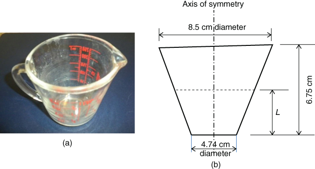
Figure 10.18 Design of a measuring cup. (a) A measuring cup. (b) The overall dimensions of the cup.
-
10.3 In Example 8.10, we derived a nonlinear equation for the amplitude of the mass attached to a spring in resonant vibration as Equation (m) in that example of the form
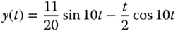
where y(t) is the amplitude of the vibrating mass at time t. Use the Newton–Raphson method to find the time te, at which the spring reaches the breaking stretching extent of 0.005 m.
-
10.4 Use the three numerical integration methods—the trapezoidal rule, Simpson's one-third rule, and Gaussian quadrature with two-sampling points—to determine the values of the following three integrals:
- a.
- b.

- c.

- a.
-
10.5 Use the three numerical integration methods—the trapezoidal rule, Simpson's one-third rule, and Gaussian quadrature with two-sampling points—to determine the plane area of a plate in the form of an ellipse as shown in Figure 10.19.

Figure 10.19 Plane area of an ellipse.
-
10.6 Derive the second-order derivative of the function f(x) as shown in Equation 10.23 for the “backward difference” scheme, and also for the “central difference scheme.”
-
10.7 Use the backward and central difference schemes to solve the differential equation in Example 10.12.
-
10.8 Use the forward difference scheme to solve the differential equation derived for the modeling of the vibration of a metal stamping machine in Example 8.9. Compare your results obtained from this finite-difference approximation and the exact solution given in the example.
-
10.9 Use both second-order and fourth-order Runge–Kutta methods to solve the first-order differential equation, Equation (7.13), for the instantaneous water level h(t) in a straight-sided cylindrical tank:
with
 ,
,  inches,
  inch, and initial water level
  inches. Compare your result at two solution points with that from Equation (7.14).
 -
10.10 Use the forward difference scheme to solve the following differential equation with a step size of
 and with prescribed conditions
  and
and  .
.
You need to present the formulations for each solution step for a total of three steps.
-
10.11 Use the fourth-order Runge–Kutta method to solve the same equation in Problem 10.10 with the same step size. Compare your results obtained from these two methods.
-
10.12 Use the fourth-order Runge–Kutta method to solve the following differential equation in Equation (a) in Example 8.10:
with
 and
and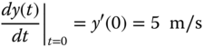
Compare your result with the exact solution of y(2) = 0.25 cm obtained from the analytical solution of the same equation as indicated in Example 8.10.