Building Neural Networks with Keras and TensorFlow

Creating a neural network using Keras’s sequential API is simple. You first create an instance of the Sequential class. Then you call add on the Sequential object to add layers. The layers are instances of classes such as Dense, which represents a fully connected layer with a specified number of neurons. The following statements create the three-layer network featured in Chapter 8:

from tensorflow.keras.models import Sequential
from tensorflow.keras.layers import Dense

model = Sequential()
model.add(Dense(3, activation='relu', input_dim=2))
model.add(Dense(1))

This network contains an input layer with two neurons, a hidden layer with three neurons, and an output layer with one neuron. Values passed from the hidden layer to the output layer are transformed by the rectified linear units (ReLU) activation function, which, you’ll recall, turns negative numbers into 0s and helps the model fit to nonlinear datasets. Observe that you don’t have to add the input layer explicitly. The input_dim=2 parameter in the first hidden layer implicitly creates an input layer with two neurons.

Once all the layers are added, the next step is to call compile and specify important attributes such as which optimizer and loss function to use during training. Here’s an example:

model.compile(optimizer='adam', loss='mae', metrics=['mae'])

Let’s walk through the parameters one at a time:

optimizer='adam'

Tells Keras to use the Adam optimizer to adjust weights and biases in each backpropagation pass during training. Adam is one of eight optimizers built into Keras, and it is among the most advanced. It employs an adaptive learning rate and is always the one I start with in the absence of a compelling reason to do otherwise.

loss='mae'

Tells Keras to use mean absolute error (MAE) to measure loss. This is common for neural networks intended to solve regression problems. Another frequently used option for regression models is loss='mse' for mean squared error (MSE).

metrics=['mae']

Tells Keras to capture MAE values as the network is trained. This information is used after training is complete to judge the efficacy of the training.

String values such as 'adam' and 'mae' are shortcuts for functions built into Keras. For example, optimizer='adam' is equivalent to optimizer=Adam(). The longhand form is useful for calling the function with nondefault parameter values—for example, optimizer=Adam(learning_rate=2e-5) to create an Adam optimizer with a custom learning rate. You’ll see an example of this in Chapter 13 when we fine-tune a model by training it with a low learning rate.

Inside the compile method, Keras creates a TensorFlow object graph to speed execution. Once the network is compiled, you train it by calling fit:

hist = model.fit(x, y, epochs=100, batch_size=100, validation_split=0.2)

The fit method accepts many parameters. Here are the ones used in this example:

x

The dataset’s feature columns.

y

The dataset’s label column—the one containing the values the network will attempt to predict.

epochs=100

Tells Keras to train the network for 100 iterations, or epochs. In each epoch, all of the training data passes through the network one time.

batch_size=100

Tells Keras to pass 100 training samples through the network before making a backpropagation pass to adjust the weights and biases. Training takes less time if the batch size is large, but accuracy could suffer. You typically experiment with different batch sizes to find the right balance between training time and accuracy. Do not assume that lowering the batch size will improve accuracy. It frequently does, but sometimes does not.

validation_split=0.2

Tells Keras that in each epoch, it should train with 80% of the rows in the dataset and validate the network’s accuracy with the remaining 20%. If you prefer, you can split the dataset yourself and use the validation_data parameter to pass the validation data to fit. Keras doesn’t offer an explicit function for splitting a dataset, but you can use Scikit’s train_test_split function to do it. One difference between train_test_split and validation_split is that the former splits the data randomly and includes an option for performing a stratified split. validation_split, by contrast, simply divides the dataset into two partitions and does not attempt to shuffle or stratify. Don’t use validation_split on ordered data without shuffling the data first.

It might surprise you to learn that if you train the same network on the same dataset several times, the results will be different each time. By default, weights are initialized with random values, and different starting points produce different outcomes. Additional randomness baked into the training process means the network will train differently even if it’s initialized with the same random weights. Rather than fight it, data scientists learn to “embrace the randomness.” If you work the tutorial in the next section, your results will differ from mine. They shouldn’t differ by a lot, but they will differ.

You judge the efficacy of training by examining information returned by the fit method. fit returns a history object containing the training and validation metrics specified in the metrics parameter passed to the compile method. For example, metrics=['mae'] captures MAE at the end of each epoch. Charting these metrics lets you determine whether you trained for the right number of epochs. It also lets you know if the network is underfitting or overfitting. Figure 9-1 plots MAE over the course of 30 training epochs.

Figure 9-1. Training and validation accuracy during training

The blue curve in Figure 9-1 reveals how the network fit to the training data. The orange curve shows how it tested against the validation data. Most of the learning was done in the first 20 epochs, but MAE continued to drop as training progressed. The validation MAE nearly matched the training MAE at the end, which is an indication that the network isn’t overfitting. You typically don’t care how well the network fits to the training data. You care about the fit to the validation data because that indicates how the network performs with data it hasn’t seen before. The greater the gap between the training and validation accuracy, the greater the likelihood that the network is overfitting.

Once a neural network is trained, you call its predict method to make a prediction:

prediction = model.predict(np.array([[2, 2]]))

In this example, the network accepts two floating-point values as input and returns a single floating-point value as output. The value returned by predict is that output.

Using a Neural Network to Predict Taxi Fares

Let’s put this knowledge to work building and training a neural network. The problem that we’ll solve is the same one presented in Chapter 2: using data from the New York City Taxi and Limousine Commission to predict taxi fares. We’ll use a neural network as a regression model to make the predictions.

Download the CSV file containing the dataset if you didn’t download it in Chapter 2 and copy it into the Data directory where your Jupyter notebooks are hosted. Then use the following code to load the dataset and show the first five rows. It contains about 55,000 rows and is a subset of a much larger dataset that was recently used in Kaggle’s New York City Taxi Fare Prediction competition:

import pandas as pd

df = pd.read_csv('Data/taxi-fares.csv', parse_dates=['pickup_datetime'])
df.head()

The data requires a fair amount of prep work before it’s useful—something that’s quite common in machine learning and in deep learning too. Use the following statements to transform the raw dataset into one suitable for training, and refer to the taxi-fare example in Chapter 2 for a step-by-step explanation of the transformations applied:

from math import sqrt

df = df[df['passenger_count'] == 1]
df = df.drop(['key', 'passenger_count'], axis=1)

for i, row in df.iterrows():
    dt = row['pickup_datetime']
    df.at[i, 'day_of_week'] = dt.weekday()
    df.at[i, 'pickup_time'] = dt.hour
    x = (row['dropoff_longitude'] - row['pickup_longitude']) * 54.6
    y = (row['dropoff_latitude'] - row['pickup_latitude']) * 69.0
    distance = sqrt(x**2 + y**2)
    df.at[i, 'distance'] = distance

df.drop(['pickup_datetime', 'pickup_longitude', 'pickup_latitude',
         'dropoff_longitude', 'dropoff_latitude'], axis=1, inplace=True)

df = df[(df['distance'] > 1.0) & (df['distance'] < 10.0)]
df = df[(df['fare_amount'] > 0.0) & (df['fare_amount'] < 50.0)]
df.head()

The resulting dataset contains columns for the day of the week (0–6, where 0 corresponds to Monday), the hour of the day (0–23), and the distance traveled in miles, and from which outliers have been removed:

The next step is to create the neural network. Use the following statements to create a network with an input layer that accepts three values (day, time, and distance), two hidden layers with 512 neurons each, and an output layer with a single neuron (the predicted fare amount):

from tensorflow.keras.models import Sequential
from tensorflow.keras.layers import Dense

model = Sequential()
model.add(Dense(512, activation='relu', input_dim=3))
model.add(Dense(512, activation='relu'))
model.add(Dense(1))
model.compile(optimizer='adam', loss='mae', metrics=['mae'])
model.summary()

The call to summary in the last statement produces a concise summary of the network topology, including the number of trainable parameters—weights and biases that can be adjusted to fit the network to a dataset (Figure 9-2). For a given layer, the parameter count is the product of the number of neurons in that layer and the previous layer (the number of weights connecting the neurons in the two layers) plus the number of neurons in the layer (the biases associated with those neurons). This network is a relatively simple one, and yet it features more than a quarter million knobs and dials that can be adjusted to fit it to a dataset.

Now separate the feature columns from the label column and use them to train the network. Set validation_split to 0.2 to validate the network using 20% of the training data. Train for 100 epochs and use a batch size of 100. Given that the dataset contains more than 38,000 samples, this means that about 380 backpropagation passes will be performed in each epoch:

x = df.drop('fare_amount', axis=1)
y = df['fare_amount']

hist = model.fit(x, y, validation_split=0.2, epochs=100, batch_size=100)

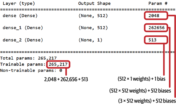
Figure 9-2. Trainable parameters in a simple neural network

Use the history object returned by fit to plot the training and validation accuracy for each epoch:

%matplotlib inline
import matplotlib.pyplot as plt
import seaborn as sns
sns.set()

err = hist.history['mae']
val_err = hist.history['val_mae']
epochs = range(1, len(err) + 1)

plt.plot(epochs, err, '-', label='Training MAE')
plt.plot(epochs, val_err, ':', label='Validation MAE')
plt.title('Training and Validation Accuracy')
plt.xlabel('Epoch')
plt.ylabel('Mean Absolute Error')
plt.legend(loc='upper right')
plt.plot()

Your results will be slightly different from mine, but they should look something like this:

The final validation MAE was about 2.25, which means that on average, a taxi fare predicted by this network should be accurate to within about $2.25.

Recall from Chapter 2 that a common accuracy measure for regression models is the coefficient of determination, or R² score. Keras doesn’t have a function for computing R² scores, but Scikit does. To that end, use the following statements to compute R² for the network:

from sklearn.metrics import r2_score

r2_score(y, model.predict(x))

Again, your results will differ from mine but will probably land at around 0.75.

Finish up by using the model to predict what it will cost to hire a taxi for a 2-mile trip at 5:00 p.m. on Friday:

import numpy as np

model.predict(np.array([[4, 17, 2.0]]))

Now predict the fare amount for a 2-mile trip taken at 5:00 p.m. one day later (on Saturday):

model.predict(np.array([[5, 17, 2.0]]))

Does the model predict a higher or lower fare amount for the same trip on Saturday afternoon? Do the results make sense given that the data comes from New York City cabs?

Before you close out this notebook, use it as a basis for further experimentation. Here are a few things you can try in order to gain further insights into neural networks:

• Run the notebook from start to finish a few times and note the differences in R² scores as well as the MAE curves. Remember that neural networks are initialized with random weights each time they’re created, and additional randomness during the training process further ensures that the results will vary from run to run.

• Vary the width of the hidden layers. I used 512 neurons in each layer and found that doing so produced acceptable results. Would 128, 256, or 1,024 neurons per layer improve the accuracy? Try it and find out. Since the results will vary slightly from one run to the next, it might be useful to train the network several times in each configuration and average the results.

• Vary the batch size. What effect does that have on training time, and why? How about the effect on accuracy?

Finally, try reducing the network to one hidden layer containing just 16 neurons. Train it again and check the R² score. Does the result surprise you? How many train­a⁠ble parameters does this network contain?

Binary Classification with Neural Networks

One of the common uses for machine learning is binary classification, which looks at an input and predicts which of two possible classes it belongs to. Practical uses include sentiment analysis, spam filtering, and fraud detection. Such models are trained with datasets labeled with 1s and 0s representing the two classes, employ popular learning algorithms such as logistic regression and Naive Bayes, and are frequently built with libraries such as Scikit-Learn.

Deep learning can be used for binary classification too. In fact, building a neural network that acts as a binary classifier is not much different than building one that acts as a regressor. In the previous section, you built a neural network that solved a regression problem. That network had an input layer that accepted three values—distance to travel, hour of the day, and day of the week—and output a predicted taxi fare. Building a neural network that performs binary classification involves making two simple changes:

• Add an activation function—specifically, the sigmoid activation function—to the output layer. sigmoid produces a value from 0.0 to 1.0 representing the probability that the input belongs to the positive class. For a reminder of what a sigmoid function does, refer to the discussion of logistic regression in Chapter 3.

• Change the loss function to binary_crossentropy, which is purpose-built for binary classifiers. Accordingly, change metrics to '[accuracy]' so that accuracies computed by the loss function are captured in the history object returned by fit.

Here’s a network designed to perform binary classification rather than regression:

from tensorflow.keras.models import Sequential
from tensorflow.keras.layers import Dense

model = Sequential()
model.add(Dense(512, activation='relu', input_dim=3))
model.add(Dense(512, activation='relu'))
model.add(Dense(1, activation='sigmoid'))
model.compile(optimizer='adam', loss='binary_crossentropy', metrics=['accuracy'])

That’s it. That’s all it takes to create a neural network that serves as a binary classifier. You still call fit to train the network, and you use the returned history object to plot the training and validation accuracy to determine whether you trained for a sufficient number of epochs and see how well the network fit to the data.

To sum up, you build a neural network that performs binary classification by including a single neuron with sigmoid activation in the output layer and specifying binary_crossentropy as the loss function. The output from the network is a probability from 0.0 to 1.0 that the input belongs to the positive class. Doesn’t get much simpler than that!

Making Predictions

One of the benefits of a neural network is that it can easily fit nonlinear datasets. You don’t have to worry about trying different learning algorithms as you do with conventional machine learning models; the network is the learning algorithm. As an example, consider the dataset in Figure 9-3, in which each data point consists of an x–y coordinate pair and belongs to one of two classes.

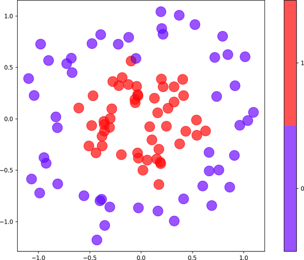
Figure 9-3. Nonlinear dataset containing two classes

The following code trains a neural network to predict a class based on a point’s x and y coordinates:

from tensorflow.keras.models import Sequential
from tensorflow.keras.layers import Dense

model = Sequential()
model.add(Dense(128, activation='relu', input_dim=2))
model.add(Dense(1, activation='sigmoid'))
model.compile(optimizer='adam', loss='binary_crossentropy', metrics=['accuracy'])
hist = model.fit(x, y, epochs=40, batch_size=10, validation_split=0.2)

This network contains just one hidden layer with 128 neurons, and yet a plot of the training and validation accuracy reveals that it is remarkably successful in separating the classes:

Once a binary classifier is trained, you make predictions by calling its predict method. Thanks to the sigmoid activation function, predict returns a number from 0.0 to 1.0 representing the probability that the input belongs to the positive class. In this example, purple data points represent the negative class (0), while red data points represent the positive class (1). Here the network is asked to predict the probability that a data point at (–0.5, 0.0) belongs to the red class:

model.predict(np.array([[-0.5, 0.0]]))

The answer is 0.57, which indicates that (–0.5, 0.0) is more likely to be red than purple. If you simply want to know which class the point belongs to, do it this way:

(model.predict(np.array([[-0.5, 0.0]])) > 0.5).astype('int32')

The answer is 1, which corresponds to red. Older versions of Keras included a predict_classes method that did the same without the astype cast, but that method was recently deprecated and removed.

Training a Neural Network to Detect Credit Card Fraud

Let’s train a neural network to detect credit card fraud. Begin by downloading a ZIP file containing the dataset if you haven’t already and copying creditcard.csv from the ZIP file into your notebooks’ Data subdirectory. It’s the same one used in Chapters 3 and 6. It contains information about 284,808 credit card transactions, including the amount of each transaction and a label: 0 for legitimate transactions and 1 for fraudulent transactions. It also contains 28 columns named V1 through V28 whose meaning has been obfuscated with principal component analysis. The dataset is highly imbalanced, containing fewer than 500 examples of fraudulent transactions.

Now load the dataset:

import pandas as pd

df = pd.read_csv('Data/creditcard.csv')
df.head(10)

Use the following statements to drop the Time column, divide the dataset into features x and labels y, and split the dataset into two datasets: one for training and one for testing. Rather than allow Keras to do the split for us, we’ll do it ourselves so that we can later run the test data through the network and use a confusion matrix to analyze the results:

from sklearn.model_selection import train_test_split

x = df.drop(['Time', 'Class'], axis=1)
y = df['Class']

x_train, x_test, y_train, y_test = train_test_split(
    x, y, test_size=0.2, stratify=y, random_state=0)

Create a neural network for binary classification:

from tensorflow.keras.models import Sequential
from tensorflow.keras.layers import Dense

model = Sequential() 
model.add(Dense(128, activation='relu', input_dim=29))
model.add(Dense(1, activation='sigmoid')) 
model.compile(loss='binary_crossentropy', optimizer='adam', metrics=['accuracy']) 
model.summary()

The next step is to train the model. Notice the validation_data parameter passed to fit, which uses the test data split off from the larger dataset to assess the model’s accuracy as training takes place:

hist = model.fit(x_train, y_train, validation_data=(x_test, y_test),
                 epochs=10, batch_size=100)

Now plot the training and validation accuracy using the per-epoch values in the history object:

%matplotlib inline
import matplotlib.pyplot as plt
import seaborn as sns
sns.set()

acc = hist.history['accuracy']
val = hist.history['val_accuracy']
epochs = range(1, len(acc) + 1)

plt.plot(epochs, acc, '-', label='Training accuracy')
plt.plot(epochs, val, ':', label='Validation accuracy')
plt.title('Training and Validation Accuracy')
plt.xlabel('Epoch')
plt.ylabel('Accuracy')
plt.legend(loc='lower right')
plt.plot()

The result looked like this for me. Remember that your results will be different thanks to the randomness inherent to training neural networks:

On the surface, the validation accuracy (around 0.9994) appears to be very high. But remember that the dataset is imbalanced. Fraudulent transactions represent less than 0.2% of all the samples, which means that the model could simply guess that every transaction is legitimate and get it right about 99.8% of the time. Use a confusion matrix to visualize how the model performs during testing with data it wasn’t trained with:

from sklearn.metrics import ConfusionMatrixDisplay as cmd

sns.reset_orig()
y_predicted = model.predict(x_test) > 0.5
labels = ['Legitimate', 'Fraudulent']

cmd.from_predictions(y_test, y_predicted, display_labels=labels,
                     cmap='Blues', xticks_rotation='vertical')

Here’s how it turned out for me:

Your results will probably vary. Indeed, train the model several times and you’ll get different results each time. In this run, the model correctly identified 56,858 transactions as legitimate while misclassifying legitimate transactions just six times. This means legitimate transactions are classified correctly about 99.99% of the time. Meanwhile, the model caught more than 73% of the fraudulent transactions. That’s acceptable, because credit card companies would rather allow 100 fraudulent transactions to go through than decline one legitimate transaction.

Note

Data scientists often use three datasets, not two, to train and assess the accuracy of a neural network: a training dataset for training, a validation dataset for validating the network (and scoring its progress) as training takes place, and a test dataset for evaluating the network’s accuracy once training is complete.

The preceding example used the same dataset for validation and testing—the 20% split off from the original dataset with train_test_split. That’s ostensibly fine because validation data is not used to adjust the network’s weights and biases during training. However, if you really want to have confidence in the network’s accuracy, it is never a bad idea to test it with a third dataset not used for training or validation. In the real world, the ultimate test of a deep-learning model’s accuracy is how it performs against data that it has never seen before.

A final note regarding this example has to do with an extra parameter you can pass to the fit method that is particularly useful when dealing with imbalanced datasets. As an experiment, try replacing the call to fit with the following statement:

hist = model.fit(x_train, y_train, validation_data=(x_test, y_test), epochs=10,
                 batch_size=100, class_weight={ 0: 1.0, 1: 0.01 })

Then run the notebook again from start to finish. In all likelihood, the resulting confusion matrix will show zero (or at most, one or two) misclassified legitimate transactions, but the percentage of correctly identified fraudulent transactions will decrease too. The class_weight parameter in this example tells the model that you care a lot more about classifying legitimate samples correctly than correctly identifying fraudulent samples. You can experiment with different weights for the two classes and find the balance that best suits the business requirements that prompted you to build the model in the first place.

Multiclass Classification with Neural Networks

Here again is a simple binary classifier that accepts two inputs, has a hidden layer with 128 neurons, and outputs a value from 0.0 to 1.0 representing the probability that the input belongs to the positive class:

from tensorflow.keras.models import Sequential
from tensorflow.keras.layers import Dense

model = Sequential()
model.add(Dense(128, activation='relu', input_dim=2))
model.add(Dense(1, activation='sigmoid'))
model.compile(optimizer='adam', loss=' binary_crossentropy',
              metrics=['accuracy'])

Key elements include an output layer with one neuron assigned the sigmoid activation function, and binary_crossentropy as the loss function. Three simple modifications repurpose this network to do multiclass classification:

from tensorflow.keras.models import Sequential
from tensorflow.keras.layers import Dense

model = Sequential()
model.add(Dense(128, activation='relu', input_dim=2))
model.add(Dense(4, activation='softmax'))
model.compile(optimizer='adam', loss='sparse_categorical_crossentropy',
              metrics=['accuracy'])

The changes are as follows:

• The output layer contains one neuron per class rather than just one neuron. If the dataset contains four classes, then the output layer has four neurons. If the dataset contains 10 classes, then the output layer has 10 neurons. Each neuron corresponds to one class.

• The output layer uses the softmax activation function rather than the sigmoid activation function. Each neuron in the output layer yields a probability for the corresponding class, and thanks to the softmax function, the sum of all the probabilities is 1.0.

• The loss function is sparse_categorical_crossentropy. During training, this loss function exponentially penalizes error in the probabilities predicted by a multiclass classifier, just as binary_crossentropy does for binary classifiers.

After defining the network, you call fit to train it and predict to make predictions. Since an example is worth a thousand words, let’s fit a neural network to a two-dimensional dataset comprising four classes (Figure 9-4).

Figure 9-4. Nonlinear dataset containing four classes

The following code trains a neural network to predict a class based on a point’s x and y coordinates:

from tensorflow.keras.models import Sequential
from tensorflow.keras.layers import Dense

model = Sequential()
model.add(Dense(128, activation='relu', input_dim=2))
model.add(Dense(4, activation='softmax'))
model.compile(optimizer='adam', loss='sparse_categorical_crossentropy',
              metrics=['accuracy'])

hist = model.fit(x, y, epochs=40, batch_size=10, validation_split=0.2)

A plot of the training and validation accuracy reveals that the network had little trouble separating the classes:

You make predictions by calling the classifier’s predict method. For each input, predict returns an array of probabilities—one per class. The predicted class is the one assigned the highest probability. In this example, purple data points represent class 0, light blue represent class 1, taupe represent class 2, and red represent class 3. Here the network is asked to classify a point that lies at (0.2, 0.8):

model.predict(np.array([[0.2, 0.8]]))

The answer is an array of four probabilities corresponding to classes 0, 1, 2, and 3, in that order:

[2.1877741e-02, 5.3804164e-05, 5.0240371e-02, 9.2782807e-01]

The network predicted there’s a 2% chance that (0.2, 0.8) corresponds to class 0, a 0% chance that it corresponds to class 1, a 5% chance that it corresponds to class 2, and a 93% chance that it corresponds to class 3. Looking at the plot, that seems like a reasonable answer.

If you simply want to know which class the point belongs to, you can do it this way:

np.argmax(model.predict(np.array([[0.2, 0.8]])), axis=1)

The answer is 3, which corresponds to red. Older versions of Keras included a predict_classes method that did the same without the call to argmax, but that method has since been deprecated and removed.

Training a Neural Network to Recognize Faces

Chapter 5 documented the steps for training a support vector machine to recognize faces. Let’s train a neural network to do the same. We’ll use the same dataset as before: the Labeled Faces in the Wild (LFW) dataset, which contains more than 13,000 facial images of famous people and is built into Scikit as a sample dataset. Recall that of the more than 5,000 people represented in the dataset, 1,680 have two or more facial images, while only 5 have 100 or more. We’ll set the minimum number of faces per person to 100, which means that five sets of faces corresponding to five famous people will be imported.

Start by creating a new Jupyter notebook and using the following statements to load the dataset:

import pandas as pd
from sklearn.datasets import fetch_lfw_people

faces = fetch_lfw_people(min_faces_per_person=100, slice_=None)
faces.images = faces.images[:, 35:97, 39:86]
faces.data = faces.images.reshape(faces.images.shape[0], faces.images.shape[1] *
                                  faces.images.shape[2])
image_count = faces.images.shape[0]
image_height = faces.images.shape[1]
image_width = faces.images.shape[2]
class_count = len(faces.target_names)

In total, 1,140 facial images were loaded. After cropping, each measures 47 × 62 pixels. Use the following code to show the first 24 images in the dataset and the people to whom the faces belong:

%matplotlib inline
import matplotlib.pyplot as plt

fig, ax = plt.subplots(3, 8, figsize=(18, 10))
for i, axi in enumerate(ax.flat):
    axi.imshow(faces.images[i], cmap='gist_gray')
    axi.set(xticks=[], yticks=[], xlabel=faces.target_names[faces.target[i]])

Check the balance in the dataset by generating a histogram showing how many facial images were imported for each person:

from collections import Counter
import seaborn as sns
sns.set()

counts = Counter(faces.target)
names = {}

for key in counts.keys():
    names[faces.target_names[key]] = counts[key]

df = pd.DataFrame.from_dict(names, orient='index')
df.plot(kind='bar')

There are far more images of George W. Bush than of anyone else in the dataset. Classification models are best trained with balanced datasets. Use the following code to reduce the dataset to 100 images of each person:

import numpy as np

mask = np.zeros(faces.target.shape, dtype=bool)

for target in np.unique(faces.target):
    mask[np.where(faces.target == target)[0][:100]] = 1

x_faces = faces.data[mask]
y_faces = faces.target[mask]
x_faces.shape

x_faces contains 500 facial images, and y_faces contains the labels that go with them: 0 for Colin Powell, 1 for Donald Rumsfeld, and so on.

The next step is to split the data for training and testing. We’ll set aside 20% of the data for testing, let Keras use it to validate the model during training, and later use it to assess the results with a confusion matrix:

from sklearn.model_selection import train_test_split

x_train, x_test, y_train, y_test = train_test_split(
    face_images, y_faces, train_size=0.8, stratify=y_faces, random_state=0)

Create a neural network containing one hidden layer with 512 neurons. Use sparse_categorical_crossentropy as the loss function and softmax as the activation function in the output layer since this is a multiclass classification task:

from tensorflow.keras.layers import Dense
from tensorflow.keras.models import Sequential

model = Sequential()
model.add(Dense(512, activation='relu',
                input_shape=(image_width * image_height,)))
model.add(Dense(class_count, activation='softmax'))
model.compile(optimizer='adam', loss='sparse_categorical_crossentropy',
              metrics=['accuracy'])
model.summary()

Now train the network:

hist = model.fit(x_train, y_train, validation_data=(x_test, y_test),
                 epochs=100, batch_size=20)

Plot the training and validation accuracy:

acc = hist.history['accuracy']
val_acc = hist.history['val_accuracy']
epochs = range(1, len(acc) + 1)

plt.plot(epochs, acc, '-', label='Training Accuracy')
plt.plot(epochs, val_acc, ':', label='Validation Accuracy')
plt.title('Training and Validation Accuracy')
plt.xlabel('Epoch')
plt.ylabel('Accuracy')
plt.legend(loc='lower right')
plt.plot()

Finally, use a confusion matrix to visualize how the network performs against test data:

from sklearn.metrics import ConfusionMatrixDisplay as cmd

sns.reset_orig()
y_pred = model.predict(x_test)
fig, ax = plt.subplots(figsize=(5, 5))
ax.grid(False)

cmd.from_predictions(y_test, y_pred.argmax(axis=1),
                     display_labels=faces.target_names, colorbar=False,
                     cmap='Blues', xticks_rotation='vertical', ax=ax)

How many times did the model correctly identify George W. Bush? How many times did it identify him as someone else? Would the network be just as accurate with 128 neurons in the hidden layer as it is with 512?

Dropout

The goal of any machine learning model is to make accurate predictions. In a perfect world, the gap between training accuracy and validation accuracy would be close to 0 in the later stages of training a neural network. In the real world, it rarely happens that way. Training accuracy for the model in the previous section approached 100%, but validation accuracy probably peaked between 80% and 85%. This means the model isn’t generalizing as well as you’d like. It learned the training data very well, but when presented with data it hadn’t seen before (the validation data), it underperformed. This may be a sign that the model is overfitting. In the end, it’s not training accuracy that matters; it’s how accurately the model responds to new data.

One way to combat overfitting is to reduce the depth of the network, the width of individual layers, or both. Fewer neurons means fewer trainable parameters, and fewer parameters makes it harder for the network to fit too tightly to the training data.

Another way to guard against overfitting is to introduce dropout to the network. Dropout randomly drops connections between layers during training to prevent the network from learning the training data too well. It’s like reading a book but skipping every other page in hopes that you’ll learn high-level concepts without getting bogged down in the details. Dropout was introduced in a 2014 paper titled “Dropout: A Simple Way to Prevent Neural Networks from Overfitting”.

Keras’s Dropout class makes adding dropout to a network dead-simple. To demonstrate, go back to the example in the previous section and redefine the network this way:

from tensorflow.keras.layers import Dense, Dropout
from tensorflow.keras.models import Sequential

model = Sequential()
model.add(Dense(512, activation='relu',
                input_shape=(image_width * image_height,)))
model.add(Dropout(0.2))
model.add(Dense(class_count, activation='softmax'))
model.compile(optimizer='adam', loss='sparse_categorical_crossentropy',
              metrics=['accuracy'])

Now train the network again and plot the training and validation accuracy. Here’s how it turned out for me:

The gap didn’t close much (if at all), but sometimes adding dropout in this manner will increase the validation accuracy. The key statement in this example is model.add(Dropout(0.2)), which adds a Dropout layer that randomly drops (ignores) 20% of the connections between the neurons in the hidden layer and the neurons in the output layer in each backpropagation pass. You can be more aggressive by dropping more connections—increasing 0.2 to 0.4, for example—but you can also reach a point of diminishing returns. Note that if you’re super-aggressive with the dropout rate (for example, 0.5), you’ll probably need to train the model for more epochs. Making it harder to learn means taking longer to learn too.

In practice, the only way to know whether dropout will improve a model’s ability to generalize is to try it. In addition to trying different dropout percentages, you can try introducing dropout between two or more layers in hopes of finding a combination that works.

Saving and Loading Models

In Chapter 7, you learned how to serialize (save) a trained Scikit model and load it in a client app. The same requirement applies to neural networks: you need a way to save a trained network and load it later in order to operationalize it.

You can get the weights and biases from a model with Keras’s get_weights method, and you can restore them with set_weights. But saving a trained model so that you can re-create it later requires an additional step. Specifically, you must save the network architecture: the number of and types of layers, the number of neurons in each layer, the activation functions used in each layer, and so on. Fortunately, all that requires just one line of code. That line of code differs depending on which of two formats you want the model saved in:

model.save('my_model.h5') # Save the model in Keras's H5 format
model.save('my_model')    # Save the model in TensorFlow's native format

Loading a saved model is equally simple:

from tensorflow.keras.models import load_model

model = load_model('my_model.h5') # Load model saved in H5 format
model = load_model('my_model') # Load model saved in TensorFlow format

Saving the model in H5 format produces a single .h5 file that encapsulates the entire model. Saving it in TensorFlow’s native format, also known as the SavedModel format, produces a series of files and subdirectories containing the serialized model. Google recommends using the latter, although it’s still common to see Keras’s H5 format used. There is no functional difference between the two, but .h5 files can only be read by Keras apps written in Python, while models saved in SavedModel format can be loaded by other frameworks. Apps written in C# with Microsoft’s ML.NET, for example, can load models saved in SavedModel format regardless of the programming language in which the model was crafted.

Once a saved model is loaded, it acts identically to the original. The predictions that it makes, for example, are identical to the predictions made by the original model. You can even further train the model by running additional training samples through it. This highlights one of the major differences between neural networks and traditional machine learning models built with Scikit. Since the state of a network is defined by its weights and biases and loading a model restores the weights and biases, neural networks inherently support incremental training, also known as continual learning, so that they can become smarter over time. Most Scikit models do not because serializing the models doesn’t save the internal state accumulated as training takes place.

To recap: you can run a million training samples through a neural network, save it, load it, and run another million training samples through it and the network picks up right where it left off. The results are identical to running 2 million training samples through the network to begin with save for minor differences that result from the randomness that is always inherent to training.

Keras Callbacks

As you train a neural network and it achieves peak validation accuracy, the peak is hard to capture. Rather than nicely level out in later epochs, the validation accuracy may go down or oscillate between peaks and valleys. Given the stochastic (random) nature of neural networks, if you mark the epoch that achieved maximum validation accuracy and train again for exactly that number of epochs, you won’t get the same results the second time. How do you train for exactly the right number of epochs to produce the best (most accurate) network possible?

An elegant solution is Keras’s callbacks API, which lets you write callback functions that are called at various points during training—for example, at the end of each epoch—and that have the ability to alter and even stop the training process. Here’s an example that creates a child class named StopCallback that inherits from Keras’s Callback class. The child class implements the on_epoch_end function that’s called at the end of each training epoch and stops training if the validation accuracy reaches 95%:

from tensorflow.keras.callbacks import Callback

class StopCallback(Callback):
    accuracy_threshold = None
    
    def __init__(self, threshold):
        self.accuracy_threshold = threshold
        
    def on_epoch_end(self, epoch, logs=None):
        if (logs.get('val_accuracy') >= self.accuracy_threshold):
            self.model.stop_training = True

callback = StopCallback(0.95)
model.fit(x, y, validation_split=0.2, epochs=100, batch_size=20,
          callbacks=[callback])
model.save('best_model.h5')

Note the validation accuracy threshold (0.95) passed to StopCallback’s constructor. The call to fit ostensibly trains the network for 100 epochs, but if the validation accuracy reaches 0.95 before that, training stops in its tracks. The final statement saves the model that achieved that accuracy.

on_epoch_end is one of several functions you can implement in classes that inherit from Callback to receive a callback when a predetermined checkpoint is reached in the training process. Others include on_epoch_begin, on_train_begin, on_train_end, on_train_batch_begin, and on_train_batch_end. You’ll find a complete list, along with examples, in “Writing Your Own Callbacks” in the Keras documentation.

In addition to providing a base Callback class from which you can create your own callback classes, Keras provides several callback classes of its own. One of them is the EarlyStopping class, which lets you stop training based on a specified criterion such as decreasing validation accuracy or increasing training loss without writing a lot of code. In the following example, training stops early if the validation accuracy fails to improve for five consecutive epochs (patience=5). When training is halted, the network’s weights and biases are automatically restored to what they were when validation accuracy peaked in the final five epochs (restore_best_weights=True):

from tensorflow.keras.callbacks import EarlyStopping

callback = EarlyStopping(monitor='val_accuracy', patience=5,
                         restore_best_weights=True)
model.fit(x, y, validation_split=0.2, epochs=100, batch_size=20,
          callbacks=[callback])

Stopping the training process based on rising training loss rather than decreasing validation accuracy at the end of each epoch requires a minor code change:

from tensorflow.keras.callbacks import EarlyStopping

callback = EarlyStopping(monitor='loss', patience=5, restore_best_weights=True)
model.fit(x, y, validation_split=0.2, epochs=100, batch_size=20,
          callbacks=[callback])

The callback that is used perhaps more than any other is ModelCheckpoint, which saves a model at specified intervals during training or, if you set save_best_only to True, saves the most accurate model. The next example trains a model for 100 epochs and saves the one that exhibits the highest validation accuracy in best_model.h5:

from tensorflow.keras.callbacks import ModelCheckpoint

callback = ModelCheckpoint(filepath='best_model.h5', monitor='val_accuracy',
                           save_best_only=True)
model.fit(x, y, validation_split=0.2, epochs=100, batch_size=20,
          callbacks=[callback])

Another frequently used callback is TensorBoard, which logs a variety of information to a specified location in the filesystem as a model is trained. The following example logs to the logs subdirectory of the current directory:

from tensorflow.keras.callbacks import TensorBoard

callback = TensorBoard(log_dir='logs', histogram_freq=1)
model.fit(x_train, y_train, validation_split=0.2, epochs=100, batch_size=20,
          callbacks=[callback])

You can use a tool called TensorBoard to monitor accuracy and loss, changes in the model’s weights and biases, and more while training takes place or after it has completed. You can launch TensorBoard from a Jupyter notebook and point it to the logs subdirectory with a command like this one:

%tensorboard --logdir logs

Or you can launch it from a command prompt by executing the same command without the percent sign. Then point your browser to http://localhost:6006 to open the TensorBoard console (Figure 9-5). “Get Started with TensorBoard” in the TensorFlow documentation contains a helpful tutorial on the basics of TensorBoard. It’s an indispensable tool in the hands of professionals, especially when training complex models that require hours, days, or even weeks to fully train.

Figure 9-5. TensorBoard showing the results of training a neural network

Other Keras callback classes include LearningRateScheduler for adjusting the learning rate at the beginning of each epoch and CSV​Log⁠ger for capturing the results of each training epoch in a CSV file. Refer to the callbacks API documentation for a complete list. In addition, observe that the fit method’s callbacks parameter is a Python list, which means you can specify multiple callbacks when you train a model. You could use one callback to stop training if certain conditions are met, for example, and another callback to log training metrics in a CSV file.

Summary

Keras and TensorFlow are widely used open source frameworks that facilitate building, training, saving, loading, and consuming (making predictions with) neural networks. You can build neural networks in a variety of programming languages using native TensorFlow APIs, but Keras abstracts those APIs and makes deep learning much more approachable. Keras apps are written in Python.

Neural networks, like traditional machine learning models, can be used to solve regression problems and classification problems. A network that performs regression has one neuron in the output layer with no activation function; the output from the network is a floating-point number. A network that performs binary classification also has one neuron in the output layer, but the sigmoid activation function ensures that the output is a value from 0.0 to 1.0 representing the probability that the input represents the positive class. For multiclass classification, the number of neurons in the output layer equals the number of classes the network can predict. The softmax activation function transforms the raw values assigned to the output neurons into an array of probabilities for each class.

When you find that a neural network is fitting too tightly to the training data, one way to combat overfitting and increase the network’s ability to generalize is to reduce the complexity of the network: reduce the number of layers, the number of neurons in individual layers, or both. Another approach is to add dropout to the network. Dropout purposely impedes a network’s ability to learn the training data by randomly ignoring a subset of the connections between layers when updating weights and biases.

Keras’s callbacks API lets you customize the training process. By processing the callbacks that occur at the end of each training epoch, for example, you can check the model’s accuracy and halt training if it has reached an acceptable level. Keras also includes a simple and easy-to-use API for saving and loading trained models. This is essential for operationalizing the models that you train—deploying them to production and using the predictive powers developed during training.

The facial recognition model in this chapter exceeded 80% in validation accuracy, but modern deep-learning models often achieve 99% accuracy on the same dataset. It won’t surprise you to learn that there is more to deep learning than multilayer perceptrons. We’ll take a deep dive into facial recognition in Chapter 11, but first we’ll explore a different type of neural network—one that’s particularly adept at solving computer-vision problems. It’s called the convolutional neural network, and it is the subject of Chapter 10.