
Chapter 13. Natural Language Processing
It’s not difficult to use Scikit-Learn to build machine learning models that analyze text for sentiment, identify spam, and classify text in other ways. But today, state-of-the-art text classification is most often performed with neural networks. You already know how to build neural networks that accept numbers and images as input. Let’s build on that to learn how to construct deep-learning models that process text—a segment of deep learning known as natural language processing, or NLP for short.
NLP encompasses a variety of activities including text classification, named-entity recognition, keyword extraction, question answering, and language translation. The accuracy of NLP models has improved in recent years for a variety of reasons, not the least of which are newer and better ways of converting words and sentences into dense vector representations that incorporate meaning, and a relatively new neural network architecture called the transformer that can zero in on the most meaningful words and even differentiate between different meanings of the same word.
One element that virtually all neural networks that process text have in common is an embedding layer, which uses word embeddings to transform arrays, or sequences, of scalar values representing words into arrays of floating-point numbers called word vectors. These vectors encode information about the meanings of words and the relationships between them. Output from an embedding layer can be input to a classification layer, or it can be input to other types of neural network layers to tease more meaning from it before subjecting it to further processing.
Transformers? Embedding layers? Word vectors? There’s a lot to unpack here, but once you wrap your head around a few basic concepts, neural networks that process language are pure magic. Let’s dive in. We’ll start by learning how to prepare text for processing by a deep-learning model and how to create word embeddings. Then we’ll put that knowledge to work building neural networks that classify text, translate text from one language to another, and more—all classic applications of NLP.
Text Preparation
Chapter 4 introduced Scikit-Learn’s CountVectorizer class, which converts rows of text into rows of word counts that a machine learning model can consume. CountVectorizer also converts characters to lowercase, removes numbers and punctuation symbols, and optionally removes stop words—common words such as and and the that are likely to have little influence on the outcome.
Text must be cleaned and vectorized before it’s used to train a neural network too, but vectorization is typically performed differently. Rather than create a table of word counts, you create a table of sequences containing tokens representing individual words. Tokens are often indices into a dictionary, or vocabulary, built from the corpus of words in the dataset. To help, Keras provides the Tokenizer class, which you can think of as the deep-learning equivalent of CountVectorizer. Here’s an example that uses Tokenizer to create sequences from four lines of text:
fromtensorflow.keras.preprocessing.textimportTokenizerlines=['The quick brown fox','Jumps over $$$ the lazy brown dog','Who jumps high into the blue sky after counting 123','And quickly returns to earth']tokenizer=Tokenizer()tokenizer.fit_on_texts(lines)sequences=tokenizer.texts_to_sequences(lines)
fit_on_texts creates a dictionary containing all the words in the input text. texts_to_sequences returns a list of sequences, which are simply arrays of indices into the dictionary:
[[1, 4, 2, 5],
 [3, 6, 1, 7, 2, 8],
 [9, 3, 10, 11, 1, 12, 13, 14, 15, 16],
 [17, 18, 19, 20, 21]]
The word brown appears in lines 1 and 2 and is represented by the index 2. Therefore, 2 appears in both sequences. Similarly, a 3 representing the word jumps appears in sequences 2 and 3. The index 0 isn’t used to denote words; it’s reserved to serve as padding. More on this in a moment.
You can use Tokenizer’s sequences_to_texts method to reverse the process and convert the sequences back into text:
['the quick brown fox',
 'jumps over the lazy brown dog',
 'who jumps high into the blue sky after counting 123',
 'and quickly returns to earth']
One revelation that comes from this is that Tokenizer converts text to lowercase and removes symbols, but it doesn’t remove stop words or numbers. If you want to remove stop words, you can use a separate library such as the Natural Language Toolkit (NLTK). You can also remove words containing numbers while you’re at it:
fromtensorflow.keras.preprocessing.textimportTokenizerfromnltk.tokenizeimportword_tokenizefromnltk.corpusimportstopwordslines=['The quick brown fox','Jumps over $$$ the lazy brown dog','Who jumps high into the blue sky after counting 123','And quickly returns to earth']defremove_stop_words(text):text=word_tokenize(text.lower())stop_words=set(stopwords.words('english'))text=[wordforwordintextifword.isalpha()andnotwordinstop_words]return' '.join(text)lines=list(map(remove_stop_words,lines))tokenizer=Tokenizer()tokenizer.fit_on_texts(lines)tokenizer.texts_to_sequences(lines)
The resulting sequences look like this:
[[3, 1, 4],
 [2, 5, 1, 6],
 [2, 7, 8, 9, 10],
 [11, 12, 13]]
which, converted back to text, are as follows:
['quick brown fox',
 'jumps lazy brown dog',
 'jumps high blue sky counting',
 'quickly returns earth']
The sequences range from three to five values in length, but a neural network expects all sequences to be the same length. Keras’s pad_sequences function performs this final step, truncating sequences longer than the specified length and padding sequences shorter than the specified length with 0s:
fromtensorflow.keras.preprocessing.sequenceimportpad_sequencespadded_sequences=pad_sequences(sequences,maxlen=4)
The resulting padded sequences look like this:
array([[0,3,1,4],[2,5,1,6],[7,8,9,10],[0,11,12,13]])
Converting these sequences back to text yields this:
['quick brown fox',
 'jumps lazy brown dog',
 'high blue sky counting',
 'quickly returns earth']
By default, pad_sequences pads and truncates on the left, but you can include a padding='post' parameter if you prefer to pad and truncate on the right. Padding on the right is sometimes important when using neural networks to translate text.
Note
Removing stop words frequently has little or no effect on text classification tasks. If you simply want to remove numbers from text input to a neural network without removing stop words, create a Tokenizer this way:
tokenizer=Tokenizer(filters='!"#$%&()*+,-./:;<=>?@[\]^_` ''{|}~0123456789')
The filters parameter tells Tokenizer what characters to remove. It defaults to '!"#$%&()*+,-./:;<=>?@[\]^_`{|}~
'. This code simply adds 0–9 to the list. Note that Tokenizer does not remove apostrophes by default, but you can remove them by adding an apostrophe to the filters list.
It’s important that text input to a neural network for predictions be tokenized and padded in the same way as text input to the model for training. If you’re thinking it sure would be nice not to have to do the tokenization and sequencing manually, there is a way around it. Rather than write a lot of code, you can include a TextVectorization layer in the model. I’ll demonstrate how momentarily. But first, you need to learn about embedding layers.
Word Embeddings
Once text is tokenized and converted into padded sequences, it is ready for training a neural network. But you probably won’t get very far training on the raw padded sequences.
One of the crucial elements of a neural network that processes text is an embedding layer whose job is to convert padded sequences of word tokens into arrays of word vectors, which represent each word with an array (vector) of floating-point numbers rather than a single integer. Each word in the input text is represented by a vector in the embedding layer, and as the network is trained, vectors representing individual words are adjusted to reflect their relationship to one another. If you’re building a sentiment analysis model and words such as excellent and amazing have similar connotations, then the vectors representing those words in the embedding space should be relatively close together so that phrases such as “excellent service” and “amazing service” score similarly.
Implementing an embedding layer by hand is a complex undertaking (especially the training aspect), so Keras offers the Embedding class. With Keras, creating a trainable embedding layer requires just one line of code:
Embedding(input_dim=10000,output_dim=32,input_length=100)
In order, the three parameters passed to the Embedding function are:
-
The vocabulary size, or the number of words in the vocabulary built by
Tokenizer -
The number of dimensions m in the embedding space
-
The length n of each padded sequence
You pick the number of dimensions m, and each word gets encoded in the embedding space as an m-dimensional vector. More dimensions provide more fitting power, but also increase training time. In practice, m is usually a number from 32 to 512.
The vectors that represent individual words in an embedding layer are learned during training, just as the weights connecting neurons in adjacent dense layers are learned. If the number of training samples is sufficiently high, training the network usually creates effective vector representations of all the words. However, if you have only a few hundred training samples, the embedding layer might not have enough information to properly vectorize the corpus of text.
In that case, you can elect to initialize the embedding layer with pretrained word embeddings rather than rely on it to learn the word embeddings on its own. Several popular pretrained word embeddings exist in the public domain, including the GloVe word vectors developed by Stanford and Google’s own Word2Vec. Pretrained embeddings tend to model semantic relationships between words, recognizing, for example, that king and queen are related terms while stairs and zebra are not. While that can be beneficial, a network trained to classify text usually performs better when word embeddings are learned from the training data because such embeddings are task specific. For an example showing how to use pretrained embeddings, see “Using Pre-trained Word Embeddings” by the author of Keras.
Text Classification
Figure 13-1 shows the baseline architecture for a neural network that classifies text. Tokenized text sequences are input to the embedding layer. The output from the embedding layer is a 2D matrix of floating-point values measuring m by n, where m is the number of dimensions in the embedding space and n is the sequence length. The Flatten layer following the embedding layer “flattens” the 2D output into a 1D array suitable for input to a dense layer, and the dense layer classifies the values emitted from the flatten layer. You can experiment with different dimensions in the embedding layer and different widths of the dense layer to maximize accuracy. You can also add more dense layers if needed.

Figure 13-1. Neural network for classifying text
A neural network like the one in Figure 13-1 can be implemented this way:
fromtensorflow.keras.modelsimportSequentialfromtensorflow.keras.layersimportDense,Flatten,Embeddingmodel=Sequential()model.add(Embedding(10000,32,input_length=100))model.add(Flatten())model.add(Dense(128,activation='relu'))model.add(Dense(1,activation='sigmoid'))model.compile(optimizer='adam',loss='binary_crossentropy',metrics=['accuracy'])
One application for a neural network that classifies text is spam filtering. Chapter 4 demonstrated how to use Scikit to build a machine learning model that separates spam from legitimate emails. Let’s build an equivalent deep-learning model with Keras and TensorFlow. We’ll use the same dataset we used before: one containing 1,000 emails, half of which are spam (indicated by 1s in the label column) and half of which are not (indicated by 0s in the label column).
Begin by downloading the dataset and copying it into the Data subdirectory where your Jupyter notebooks are hosted. Then use the following statements to load the dataset and shuffle the rows to distribute positive and negative samples throughout. Shuffling is important because rather than use train_test_split to create a validation dataset, we’ll use fit’s validation_split parameter. It doesn’t shuffle the data as train_test_split does:
importpandasaspddf=pd.read_csv('Data/ham-spam.csv')df=df.sample(frac=1,random_state=0)df.head()
Use the following statements to remove any duplicate rows from the dataset and check for balance:
df=df.drop_duplicates()df.groupby('IsSpam').describe()
Next, extract the emails from the DataFrame’s Text column and labels from the IsSpam column. Then use Keras’s Tokenizer class to tokenize the text and convert it into sequences, and pad_sequences to produce sequences of equal length. There’s no need to remove stop words because doing so doesn’t impact the outcome:
fromtensorflow.keras.preprocessing.textimportTokenizerfromtensorflow.keras.preprocessing.sequenceimportpad_sequencesx=df['Text']y=df['IsSpam']max_words=10000# Limit the vocabulary to the 10,000 most common wordsmax_length=500tokenizer=Tokenizer(num_words=max_words)tokenizer.fit_on_texts(x)sequences=tokenizer.texts_to_sequences(x)x=pad_sequences(sequences,maxlen=max_length)
Define a binary classification model that contains an embedding layer with 32 dimensions, a flatten layer to flatten output from the embedding layer, a dense layer for classification, and an output layer with a single neuron and sigmoid activation:
fromtensorflow.keras.modelsimportSequentialfromtensorflow.keras.layersimportDense,Flatten,Embeddingmodel=Sequential()model.add(Embedding(max_words,32,input_length=max_length))model.add(Flatten())model.add(Dense(128,activation='relu'))model.add(Dense(1,activation='sigmoid'))model.compile(loss='binary_crossentropy',optimizer='adam',metrics=['accuracy'])model.summary()
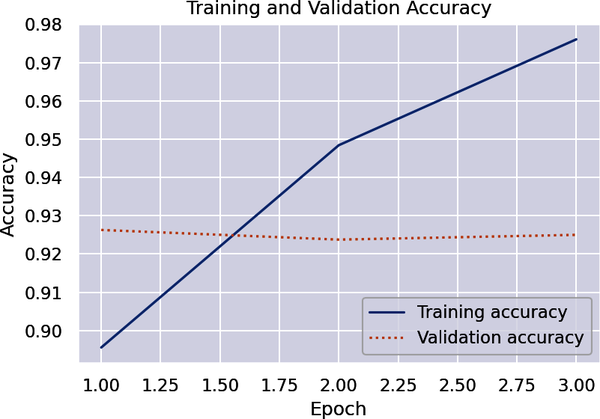
Train the network and allow Keras to use 20% of the training samples for validation:
hist=model.fit(x,y,validation_split=0.2,epochs=5,batch_size=20)
Use the history object returned by fit to plot the training and validation accuracy in each epoch:
importseabornassnsimportmatplotlib.pyplotasplt%matplotlibinlinesns.set()acc=hist.history['accuracy']val=hist.history['val_accuracy']epochs=range(1,len(acc)+1)plt.plot(epochs,acc,'-',label='Training accuracy')plt.plot(epochs,val,':',label='Validation accuracy')plt.title('Training and Validation Accuracy')plt.xlabel('Epoch')plt.ylabel('Accuracy')plt.legend(loc='lower right')plt.plot()
Hopefully, the network achieved a validation accuracy exceeding 95%. If it didn’t, train it again. Here’s how it turned out for me:

Once you’re satisfied with the accuracy, use the following statements to compute the probability that an email regarding a code review is spam:
text='Can you attend a code review on Tuesday? ''Need to make sure the logic is rock solid.'sequence=tokenizer.texts_to_sequences([text])padded_sequence=pad_sequences(sequence,maxlen=max_length)model.predict(padded_sequence)[0][0]
Then do the same for another email:
text='Why pay more for expensive meds when ''you can order them online and save $$$?'sequence=tokenizer.texts_to_sequences([text])padded_sequence=pad_sequences(sequence,maxlen=max_length)model.predict(padded_sequence)[0][0]
What did the network predict for the first email? What about the second? Do you agree with the predictions? Remember that a number close to 0.0 indicates that the email is not spam, while a number close to 1.0 indicates that it is.
Automating Text Vectorization
Rather than run Tokenizer and pad_sequences manually, you can preface an embedding layer with a TextVectorization layer. Here’s an example:
fromtensorflow.keras.modelsimportSequentialfromtensorflow.keras.layersimportDense,Flatten,Embeddingfromtensorflow.keras.layersimportTextVectorization,InputLayerimporttensorflowastfmodel=Sequential()model.add(InputLayer(input_shape=(1,),dtype=tf.string))model.add(TextVectorization(max_tokens=max_words,output_sequence_length=max_length))model.add(Embedding(max_words,32,input_length=max_length))model.add(Flatten())model.add(Dense(128,activation='relu'))model.add(Dense(1,activation='sigmoid'))model.compile(loss='binary_crossentropy',optimizer='adam',metrics=['accuracy'])model.summary()
Note that the input layer (an instance of InputLayer) is now explicitly defined, and it’s configured to accept string input. In addition, before training the model, the TextVectorization layer must be fit to the input data by calling adapt:
model.layers[0].adapt(x)
Now you no longer need to preprocess the training text, and you can pass raw text strings to predict:
text='Why pay more for expensive meds when ''you can order them online and save $$$?'model.predict([text])[0][0]
TextVectorization doesn’t remove stop words, so if you want them removed, you can do that separately or use the TextVectorization function’s standardize parameter to identify a callback function that does it for you.
Using TextVectorization in a Sentiment Analysis Model
To demonstrate how TextVectorization layers simplify text processing, let’s use it to build a binary classifier that performs sentiment analysis. We’ll use the same dataset we used in Chapter 4: the IMDB reviews dataset containing 25,000 positive reviews and 25,000 negative reviews.
Download the dataset if you haven’t already and place it in your Jupyter notebooks’ Data subdirectory. Then create a new notebook and use the following statements to load and shuffle the dataset:
importpandasaspddf=pd.read_csv('Data/reviews.csv',encoding="ISO-8859-1")df=df.sample(frac=1,random_state=0)df.head()
Remove duplicate rows and check for balance:
df=df.drop_duplicates()df.groupby('Sentiment').describe()
Now create the model and include a TextVectorization layer to preprocess input text:
fromtensorflow.keras.modelsimportSequentialfromtensorflow.keras.layersimportTextVectorization,InputLayerfromtensorflow.keras.layersimportDense,Flatten,Embeddingimporttensorflowastfmax_words=20000max_length=500model=Sequential()model.add(InputLayer(input_shape=(1,),dtype=tf.string))model.add(TextVectorization(max_tokens=max_words,output_sequence_length=max_length))model.add(Embedding(max_words,32,input_length=max_length))model.add(Flatten())model.add(Dense(128,activation='relu'))model.add(Dense(1,activation='sigmoid'))model.compile(loss='binary_crossentropy',optimizer='adam',metrics=['accuracy'])model.summary()
Extract the reviews from the DataFrame’s Text column and the labels (0 for negative sentiment, 1 for positive) from the Sentiment column, and use the former to fit the TextVectorization layer to the text. Then train the model:
x=df['Text']y=df['Sentiment']model.layers[0].adapt(x)hist=model.fit(x,y,validation_split=0.5,epochs=5,batch_size=250)
When training is complete, plot the training and validation accuracy:
importseabornassnsimportmatplotlib.pyplotasplt%matplotlibinlinesns.set()acc=hist.history['accuracy']val=hist.history['val_accuracy']epochs=range(1,len(acc)+1)plt.plot(epochs,acc,'-',label='Training accuracy')plt.plot(epochs,val,':',label='Validation accuracy')plt.title('Training and Validation Accuracy')plt.xlabel('Epoch')plt.ylabel('Accuracy')plt.legend(loc='lower right')plt.plot()
The model fits to the training text extremely well, but validation accuracy usually peaks between 85% and 90%:

Use the model to score a positive comment for sentiment:
text='Excellent food and fantastic service!'model.predict([text])[0][0]
Now do the same for a negative comment:
text='The long lines and poor customer service really turned me off.'model.predict([text])[0][0]
Observe how much simpler the code is. Operationalizing the model is simpler too, because you no longer need a Tokenizer fit to the training data to prepare text submitted to the model for predictions. Be aware, however, that a model with a TextVectorization layer can’t be saved in Keras’s H5 format. It can be saved in TensorFlow’s SavedModel format. The following statement saves the model in the saved_model subdirectory of the current directory:
model.save('saved_model')
Once the model is reloaded, you can pass text directly to it for making predictions.
Factoring Word Order into Predictions
Both of the models you just built are bag-of-words models that ignore word order. Such models are common and are often more accurate than other types of models. But that’s not always the case. The relative position of the words in a sentence sometimes has meaning. Credit and card should probably influence a spam classifier one way if they appear far apart in a sentence and another way if they appear together.
One way to improve—or at least attempt to improve—on a simple bag-of-words model is to use n-grams as described in Chapter 4. An n-gram is a collection of n words appearing in consecutive order. Keras’s TextVectorization class features an ngrams parameter that makes applying n-grams easy. The following statement creates a TextVectorization layer that considers word pairs as well as individual words:
model.add(TextVectorization(max_tokens=max_words,output_sequence_length=max_length,ngrams=2))
One limitation of n-grams is that they only consider words that are directly adjacent to each other. A slightly more robust way to factor word position into a classification task is to replace dense layers with Conv1D and MaxPooling1D layers, turning the network into a convolutional neural network. CNNs are most often used to classify images, but one-dimensional convolution layers play well with text sequences. Here’s the network presented in the previous example recast as a CNN:
fromtensorflow.keras.modelsimportSequentialfromtensorflow.keras.layersimportConv1D,MaxPooling1D,GlobalMaxPooling1Dfromtensorflow.keras.layersimportTextVectorization,InputLayerfromtensorflow.keras.layersimportDense,Embeddingimporttensorflowastfmodel=Sequential()model.add(InputLayer(input_shape=(1,),dtype=tf.string))model.add(TextVectorization(max_tokens=max_words,output_sequence_length=max_length))model.add(Embedding(max_words,32,input_length=max_length))model.add(Conv1D(32,7,activation='relu'))model.add(MaxPooling1D(5))model.add(Conv1D(32,7,activation='relu'))model.add(GlobalMaxPooling1D())model.add(Dense(1,activation='sigmoid'))model.compile(loss='binary_crossentropy',optimizer='adam',metrics=['accuracy'])
Rather than process individual words, the Conv1D layers in this example extract features from groups of vectors representing words (seven in the first layer and seven more in the second), just as Conv2D layers extract features from blocks of pixels. The MaxPooling1D layer condenses the output from the first Conv1D layer to reveal higher-level structure in input sequences, similar to the way reducing the resolution of an image tends to draw out macro features such as the shape of a person’s body while minimizing or filtering out altogether lesser features such as the shape of a person’s eyes. A simple CNN like this one sometimes classifies text more accurately than bag-of-words models, and sometimes does not. As is so often the case in machine learning, the only way to know is to try.
Recurrent Neural Networks (RNNs)
Yet another way to factor word position into a classifier is to include recurrent layers in the network. Recurrent layers were originally invented to process time-series data—for example, to look at weather data for the past five days and predict what tomorrow’s high temperature will be. If you simply took all the weather data for those five days and treated each day independently, trends evident in the data would be lost. A recurrent layer, however, might detect those trends and factor them into its output. A sequence of vectors output by an embedding layer qualifies as a time series because words in a phrase are ordered consecutively and words used early in a phrase could inform how words that occur later are interpreted.
Figure 13-2 illustrates how a recurrent layer transforms word embeddings into a vector that’s influenced by word order. In this example, sequences are input to an embedding layer, which transforms each word (token) in the sequence into a vector of floating-point numbers. These word embeddings are input to a recurrent layer, yielding another output vector. To compute that vector, cells in the recurrent layer loop over the embeddings comprising the sequence. The input to iteration n + 1 of the loop is the current embedding vector and the output from iteration n—the so-called hidden state. The output from the recurrent layer is the output from the final iteration of the loop. The result is different than it would have been had each embedding vector been processed independently because each iteration uses information from the previous iteration to compute an output. Context from a word early in a sequence can carry over to words that occur later on.

Figure 13-2. Processing word embeddings with a recurrent layer
It’s not difficult to build a very simple recurrent layer by hand that works reasonably well with short sequences (say, four or five words), but longer sequences will suffer from a vanishing-gradient effect that means words far apart will exert little influence over one another. One solution is a recurrent layer composed of Long Short-Term Memory (LSTM) cells, which were introduced in a 1997 paper titled, appropriately enough, “Long Short-Term Memory”.
LSTM cells are miniature neural networks in their own right. As the cells loop over the words in a sequence, they learn (just as the weights connecting neurons in dense layers are learned) which words are important and lend that information precedence in subsequent iterations through the loop. A dense layer doesn’t recognize that there’s a connection between blue and sky in the phrase “I like blue, for on a clear and sunny day, it is the color of the sky.” An LSTM layer does and can factor that into its output. Its power diminishes, however, as words grow farther apart.
Keras provides a handy implementation of LSTM layers in its LSTM class. It also provides a GRU class implementing gated recurrent unit (GRU) layers, which are simplified LSTM layers that train faster and often yield results that equal or exceed those of LSTM layers. Here’s how our spam classifier would look if it were modified to use LSTM:
fromtensorflow.keras.modelsimportSequentialfromtensorflow.keras.layersimportTextVectorization,InputLayerfromtensorflow.keras.layersimportDense,Embedding,LSTMimporttensorflowastfmodel=Sequential()model.add(InputLayer(input_shape=(1,),dtype=tf.string))model.add(TextVectorization(max_tokens=max_words,output_sequence_length=max_length))model.add(Embedding(max_words,32,input_length=max_length))model.add(LSTM(32))model.add(Dense(1,activation='sigmoid'))model.compile(loss='binary_crossentropy',optimizer='adam',metrics=['accuracy'])
LSTMs are compute intensive, especially when dealing with long sequences. If you try this code, you’ll find that the model takes much longer to train. You’ll also find that validation accuracy improves little if at all. This goes back to the fact that bag-of-words models, while simple, also tend to be effective at classifying text.
LSTM layers can be stacked, just like dense layers. The trick is to include a return_sequences=True attribute in all LSTM layers except the last so that the previous layers return all the vectors generated (all the hidden state) rather than just the final vector. Google Translate once used two stacks of LSTMs eight layers deep to encode phrases in one language and decode them into another.
Using Pretrained Models to Classify Text
If training your own sentiment analysis model doesn’t yield the accuracy you require, you can always turn to a pretrained model. Just as there are pretrained computer-vision models trained with millions of labeled images, there are pretrained sentiment analysis models available that were trained with millions of labeled text samples. Keras doesn’t provide a convenient wrapper around these models as it does for pretrained CNNs, but they are relatively easy to consume nonetheless.
Many such models are available from Hugging Face, an AI-focused company whose goal is to advance and democratize AI. Hugging Face originally concentrated on NLP models but has since expanded its library to include other types of models, including image classification models and object detection models. Currently, Hugging Face hosts more than 400 sentiment analysis models trained on different types of input ranging from tweets to product reviews in a variety of languages. It even offers models that analyze text for joy, anger, surprise, and other emotions.
All of these models are free for you to use. Care to give it a try? Start by installing Hugging Face’s Transformers package in your Python environment (for example, pip install transformers). Then fire up a Jupyter notebook and use the following code to load Hugging Face’s default sentiment analysis model:
fromtransformersimportpipelinemodel=pipeline('sentiment-analysis')
You’ll incur a short delay while the model is downloaded for the first time. Once the download completes, score a sentence for sentiment:
model('The long lines and poor customer service really turned me off')
Here’s the result:
[{'label': 'NEGATIVE', 'score': 0.9995430707931519}]Try it with a positive comment:
model('Great food and excellent service!')
Here’s the result:
[{'label': 'POSITIVE', 'score': 0.9998843669891357}]In the return value, label indicates whether the sentiment is positive or negative, and score reveals the model’s confidence in the label.
It’s just as easy to analyze a text string for emotion by loading a different pretrained model. To demonstrate, try this:
model=pipeline('text-classification',model='bhadresh-savani/distilbert-base-uncased-emotion',return_all_scores=True)model('The long lines and poor customer service really turned me off')
Here’s what it returned for me:
[[{'label': 'sadness', 'score': 0.10837080329656601},
  {'label': 'joy', 'score': 0.002373947761952877},
  {'label': 'love', 'score': 0.0006029471987858415},
  {'label': 'anger', 'score': 0.8861245512962341},
  {'label': 'fear', 'score': 0.0019340706057846546},
  {'label': 'surprise', 'score': 0.0005936296074651182}]]
It doesn’t get much easier than that! And as you’ll see in a moment, pretrained Hugging Face models lend themselves to much more than just text classification.
Neural Machine Translation
In the universe of natural language processing, text classification is a relatively simple task. At the opposite end of the spectrum lies neural machine translation (NMT), which uses deep learning to translate text from one language to another. NMT has proven superior to the rules-based machine translation (RBMT) and statistical machine translation (SMT) systems that predated the explosion of deep learning and today is the basis for virtually all state-of-the-art text translation services.
The gist of text classification is that you transform an input sequence into a vector characterizing the sequence, and then you input the vector to a classifier. There are several ways to generate that vector. You can reshape the 2D output from an embedding layer into a 1D vector, or you can feed that output into a recurrent layer or convolution layer in hopes of generating a vector that is more context aware. Whichever route you choose, the goal is simple: convert a string of text into an array of floating-point numbers that uniquely describes it and use a sigmoid or softmax output layer to classify it.
NMT is basically an extension of text classification. You start by converting a text sequence into a vector. But rather than classify the vector, you use it to generate a new sequence. One way to do that is with an LSTM encoder-decoder.
LSTM Encoder-Decoders
Until a few years ago, most NMT models, including the one underlying Google Translate, were LSTM-based sequence-to-sequence models similar to the one in Figure 13-3. In such models, one or more LSTM layers encode a tokenized input sequence representing the phrase to be translated into a vector. A second set of recurrent layers uses that vector as input and decodes it into a tokenized phrase in another language. The model accepts sequences as input and returns sequences as output, hence the term sequence-to-sequence model. A softmax output layer at the end outputs a set of probabilities for each token in the output sequence. If the maximum output phrase length that’s supported is 20 tokens, for example, and the vocabulary of the output language contains 20,000 words, then the output is 20 sets (one per token) of 20,000 probabilities. The word selected for each output token is the word assigned the highest probability.

Figure 13-3. LSTM-based encoder-decoder for neural machine translation
LSTM-based sequence-to-sequence models are relatively easy to build with Keras and TensorFlow. This book’s GitHub repo contains a notebook that uses 50,000 samples to train an LSTM model to translate English to French. The model is defined this way:
model=Sequential()model.add(Embedding(en_vocab_size,256,input_length=en_max_len,mask_zero=True))model.add(LSTM(256))model.add(RepeatVector(fr_max_len))model.add(LSTM(256,return_sequences=True))model.add(Dropout(0.4))model.add(TimeDistributed(Dense(fr_vocab_size,activation='softmax')))model.compile(loss='sparse_categorical_crossentropy',optimizer='adam',metrics=['accuracy'])model.summary(line_length=100)
The first layer is an embedding layer that converts word tokens into vectors containing 256 floating-point values. The mask_zero=True parameter indicates that zeros in the input sequences denote padding so that the next layer can ignore them. (There is no need to translate those tokens, after all.) Next is an LSTM layer that encodes English phrases input to the model. A second LSTM layer decodes the phrases into dense vectors representing the French equivalents. In between lies a RepeatVector layer that reshapes the output from the first LSTM layer for input to the second by repeating the output a specified number of times. The final layer is a softmax classification layer that outputs probabilities for each word in the French vocabulary. The TimeDistributed wrapper ensures that the model outputs a set of probabilities for each token in the output rather than just one set for the entire sequence.
After 34 epochs of training, the model translates 10 test phrases this way:
its fall now => cest maintenant maintenant
im losing => je suis en train
it was quite funny => cetait fut amusant amusant
thats not unusual => ce nest pas inhabituel
i think ill do that => je pense que je le
tom looks different => tom a lair different
its worth a try => ca vaut le coup
fortune smiled on him => la la lui a souri
lets hit the road => taillons la
i love winning => jadore gagner
The model isn’t perfect, in part due to the limited size of the training set. Real NMT models are trained with hundreds of millions or even billions of phrases. But is this one truly representative of the models used for state-of-the-art text translation? Figure 13-4 is adapted from an image in a 2016 paper written by Google engineers documenting the architecture of Google Translate. The architecture maps closely to that of the model just presented. It’s deeper, with eight LSTM layers in the encoder and eight in the decoder. It also employs residual connections between layers to support the network’s greater depth.

Figure 13-4. Google Translate circa 2016
One difference between our model and the model described in the paper is the block labeled “Attention” between the encoder and decoder. In deep learning, attention is a mechanism for focusing a model’s attention on the parts of a phrase that are most important, recognizing that one word can have different meanings in different contexts and that the meaning of a word sometimes depends on what’s around it.
Attention was introduced to deep learning in a seminal 2014 paper titled “Neural Machine Translation by Jointly Learning to Align and Translate”, but it wasn’t until a few years later that attention took center stage as a way to replace LSTM layers rather than supplement them. Enter perhaps the most significant contribution to the field of NMT, and to NLP overall, to date: the transformer model.
Transformer Encoder-Decoders
A landmark 2017 paper titled “Attention Is All You Need” changed the way data scientists approach NMT and other neural text processing tasks. It proposed a better way to perform sequence-to-sequence processing based on transformer models that eschew recurrent layers and use attention mechanisms to model the context in which words are used. Today transformer models have almost entirely replaced LSTM-based models.
Figure 13-5 is adapted from an image in the aforementioned paper. On the left is the encoder, which takes text sequences as input and generates dense vector representations of those sequences. On the right is the decoder, which transforms dense vector representations of input sequences into output sequences. At a high level, a transformer model uses the same encoder-decoder architecture as an LSTM-based model. The difference lies in how it does the encoding and decoding.
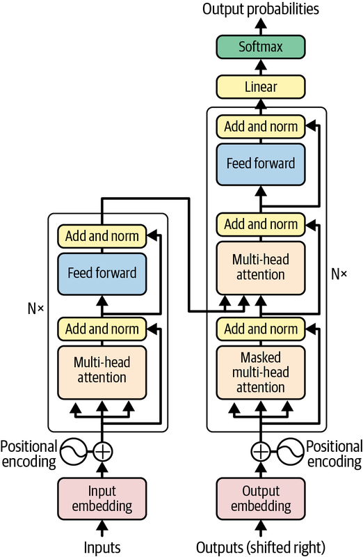
Figure 13-5. The transformer model
The chief innovation introduced by the transformer model is the use of multi-head attention (MHA) layers in place of LSTM layers. MHA layers embody the concept of self-attention, which enables a model to analyze an input sequence and focus on the words that are most important as well as the context in which the words are used. In the sentence “We took a walk in the park,” for example, the word park has a different meaning than it does in “Where did you park the car?” An embedding layer stores one vector representation for park, but in a transformer model, the MHA layer modifies the vector output by the embedding layer so that park is represented by two different vectors in the two sentences. Not surprisingly, the values used to make embedding vectors context aware are learned during training.
Note
How does self-attention work? The gist is that an MHA layer uses dot products to compute similarity scores for every word pair in a sequence. After normalizing the scores, it uses them to compute weighted versions of each word embedding in the sequence. Then it modifies them again using weights learned during training.
The “multi” in multi-head attention denotes the fact that an MHA layer learns several sets of weights rather than just one, not unlike a convolution layer in a CNN. This gives MHA the ability to discern context in long sequences where words might have multiple relationships to one another.
MHA also provides additional context regarding words that refer to other words. An embedding layer represents the pronoun it with a single vector, but an MHA layer helps the model understand that in the sentence “I love my car because it is fast,” it refers to a car. It also adds weight to the word fast because it’s crucial to the meaning of the sentence. Without it, it’s not clear why you love your car.
Unlike LSTM layers, MHA layers’ ability to model relationships among the words in an input sequence is independent of sequence length. MHA layers also support parallel workloads and therefore train faster on multiple GPUs. They do not, however, encode information regarding the positions of the words in a phrase. To compensate, a transformer uses simple vector addition to add information denoting a word’s position in a sequence to each vector output from the embedding layer. This is referred to as positional encoding or positional embedding. It’s denoted by the plus signs labeled “Positional encoding” in Figure 13-5.
Transformers aren’t limited to neural machine translation; they’re used in virtually all aspects of NLP today. The encoder half of a transformer outputs dense vector representations of the sequences input to it. Text classification can be performed by using a transformer rather than a standalone embedding layer to encode input sequences. Models architected this way frequently outperform bag-of-words models, particularly if the ratio of samples to sample length (the number of training samples divided by the average length of each sample) exceeds 1,500. This so-called “golden constant” was discovered by a team of researchers at Google and documented in a tutorial on text classification.
Building a Transformer-Based NMT Model
Keras provides some, but not all, of the building blocks that comprise an end-to-end transformer. It provides a handy implementation of self-attention layers in its MultiHeadAttention class, for example, but it doesn’t implement positional embedding. However, a separate package named KerasNLP does. Among others, it includes the following classes representing layers in a transformer-based network:
TransformerEncoder- Represents a transformer encoder
TransformerDecoder- Represents a transformer decoder
TokenAndPositionEmbedding- Implements an embedding layer that supports positional embedding
With these classes, transformer-based NMT models are relatively easy to build. You can demonstrate by building an English-to-French translator. Start by installing KerasNLP if it isn’t already installed. Then download en-fr.txt, a data file that contains 50,000 English phrases and their French equivalents, and drop it into the Data subdirectory where your Jupyter notebooks are hosted. The file en-fr.txt is a subset of a larger file containing more than 190,000 phrases and their corresponding translations compiled as part of the Tatoeba project. The file is tab delimited. Each line contains an English phrase, the equivalent French phrase, and an attribution identifying where the translation came from. We don’t need the attributions, so load the dataset into a DataFrame, remove the attribution column, and shuffle and reindex the rows:
importpandasaspddf=pd.read_csv('Data/en-fr.txt',names=['en','fr','attr'],usecols=['en','fr'],sep='')df=df.sample(frac=1,random_state=42)df=df.reset_index(drop=True)df.head()
Here’s the output:

The dataset needs to be cleaned before it’s used to train a model. Use the following statements to remove numbers and punctuation symbols, convert words with Unicode characters such as où into their ASCII equivalents (ou), convert characters to lowercase, and insert [start] and [end] tokens at the beginning and end of each French phrase:
importrefromunicodedataimportnormalizedefclean_text(text):text=normalize('NFD',text.lower())text=re.sub('[^A-Za-z ]+','',text)returntextdefclean_and_prepare_text(text):text='[start] '+clean_text(text)+' [end]'returntextdf['en']=df['en'].apply(lambdarow:clean_text(row))df['fr']=df['fr'].apply(lambdarow:clean_and_prepare_text(row))df.head()
The output looks a little cleaner afterward:

The next step is to scan the dataset and determine the maximum length of the English phrases and of the French phrases. These lengths will determine the lengths of the sequences input to and output from the model:
en=df['en']fr=df['fr']en_max_len=max(len(line.split())forlineinen)fr_max_len=max(len(line.split())forlineinfr)sequence_len=max(en_max_len,fr_max_len)(f'Max phrase length (English):{en_max_len}')(f'Max phrase length (French):{fr_max_len}')(f'Sequence length:{sequence_len}')
In this example, the longest English phrase contains seven words, while the longest French phrase contains 16 (including the [start] and [end] tokens). The model will be able to translate English phrases up to seven words in length into French phrases up to 14 words in length.
Now fit one Tokenizer to the English phrases and another Tokenizer to their French equivalents, and generate padded sequences from all the phrases. Note the filters parameter passed to the French tokenizer. It configures the tokenizer to remove all the punctuation characters it normally removes except for the square brackets used to delimit [start] and [end] tokens:
fromtensorflow.keras.preprocessing.textimportTokenizerfromtensorflow.keras.preprocessing.sequenceimportpad_sequencesen_tokenizer=Tokenizer()en_tokenizer.fit_on_texts(en)en_sequences=en_tokenizer.texts_to_sequences(en)en_x=pad_sequences(en_sequences,maxlen=sequence_len,padding='post')fr_tokenizer=Tokenizer(filters='!"#$%&()*+,-./:;<=>?@\^_`{|}~')fr_tokenizer.fit_on_texts(fr)fr_sequences=fr_tokenizer.texts_to_sequences(fr)fr_y=pad_sequences(fr_sequences,maxlen=sequence_len+1,padding='post')
Next, compute the vocabulary size for each language from the Tokenizer instances:
en_vocab_size=len(en_tokenizer.word_index)+1fr_vocab_size=len(fr_tokenizer.word_index)+1(f'Vocabulary size (English):{en_vocab_size}')(f'Vocabulary size (French):{fr_vocab_size}')
The output reveals that the English vocabulary contains 6,033 words, while the French vocabulary contains 12,197. These values will be used to size the model’s two embedding layers. The latter will also be used to size the output layer.
Finally, create the features and the labels the model will be trained with. The features are the padded English sequences and the padded French sequences minus the [end] tokens. The labels are the padded French sequences minus the [start] tokens. Package the features in a dictionary so that they can be input to a model that accepts multiple inputs:
inputs={'encoder_input':en_x,'decoder_input':fr_y[:,:-1]}outputs=fr_y[:,1:]
Now let’s define a model. This time, we’ll use Keras’s functional API rather than its sequential API. It’s necessary because this model has two inputs: one that accepts a tokenized English phrase and another that accepts a tokenized French phrase. We’ll also seed the random-number generators used by Keras and TensorFlow to get repeatable results, at least on CPU. This is a departure from all the other examples in this book, but it ensures that when you train the model, you get the same results that I did. Here’s the code:
importnumpyasnpimporttensorflowastffromtensorflow.kerasimportModelfromtensorflow.keras.layersimportInput,Dense,Dropoutfromkeras_nlp.layersimportTokenAndPositionEmbedding,TransformerEncoderfromkeras_nlp.layersimportTransformerDecodernp.random.seed(42)tf.random.set_seed(42)num_heads=8embed_dim=256encoder_input=Input(shape=(None,),dtype='int64',name='encoder_input')x=TokenAndPositionEmbedding(en_vocab_size,sequence_len,embed_dim)(encoder_input)encoder_output=TransformerEncoder(embed_dim,num_heads)(x)encoded_seq_input=Input(shape=(None,embed_dim))decoder_input=Input(shape=(None,),dtype='int64',name='decoder_input')x=TokenAndPositionEmbedding(fr_vocab_size,sequence_len,embed_dim,mask_zero=True)(decoder_input)x=TransformerDecoder(embed_dim,num_heads)(x,encoded_seq_input)x=Dropout(0.4)(x)decoder_output=Dense(fr_vocab_size,activation='softmax')(x)decoder=Model([decoder_input,encoded_seq_input],decoder_output)decoder_output=decoder([decoder_input,encoder_output])model=Model([encoder_input,decoder_input],decoder_output)model.compile(optimizer='adam',loss='sparse_categorical_crossentropy',metrics=['accuracy'])model.summary(line_length=100)
The model is designed to operate iteratively. To translate text, you first pass an English phrase to the English input and the word “[start]” to the French input. Then you append the next French word the model predicts to the previous French input and call the model again, and you repeat this process until the entire phrase has been translated—that is, until the next word predicted by the model is “[end].”
Figure 13-6 diagrams the model’s architecture. The model includes two embedding layers: one for English sequences and one for French sequences. Both convert word tokens into vectors of 256 floating point values each, and both are instances of KerasNLP’s TokenAndPositionEmbedding class, which adds positional information to word embeddings. Output from the English embedding layer passes through an encoder (an instance of TransformerEncoder) before being input along with the output from the French embedding layer to the decoder, which is an instance of TransformerDecoder. The decoder outputs a vector representing the next step in the translation, and a softmax output layer converts that vector into a set of probabilities—one for each word in the French vocabulary—identifying the next token. During training, the mask_zero=True parameter passed to the French embedding layer limits the model to making predictions based on the tokens preceding the one that’s being predicted. In other words, given a set of French tokens numbered 0 through n, the model is trained to predict what token n + 1 will be without peeking at n + 1 in the training text.

Figure 13-6. Transformer-based NMT architecture
Now call fit to train the model, and use an EarlyStopping callback to end training if the validation accuracy fails to improve for three consecutive epochs:
fromtensorflow.keras.callbacksimportEarlyStoppingcallback=EarlyStopping(monitor='val_accuracy',patience=3,restore_best_weights=True)hist=model.fit(inputs,outputs,epochs=50,validation_split=0.2,callbacks=[callback])
Training typically requires two to three minutes per epoch on CPU. If you don’t have a GPU and training is too slow, I recommend running the code in Google Colab. (Be sure to go to “Notebook settings” in the Edit menu and select GPU as the hardware accelerator.) When training is complete, plot the per-epoch training and validation accuracy and observe how the latter steadily increases until it levels off:
importseabornassnsimportmatplotlib.pyplotasplt%matplotlibinlinesns.set()acc=hist.history['accuracy']val=hist.history['val_accuracy']epochs=range(1,len(acc)+1)plt.plot(epochs,acc,'-',label='Training accuracy')plt.plot(epochs,val,':',label='Validation accuracy')plt.title('Training and Validation Accuracy')plt.xlabel('Epoch')plt.ylabel('Accuracy')plt.legend(loc='lower right')plt.plot()
The output should look like this:

The plot reveals that at the end of 14 epochs, the model was about 75% accurate in translating English samples in the validation data to French. This isn’t a very robust measure of accuracy because it literally compares each word in the predicted text to each word in the target text and ignores the fact that a missing or misplaced article such as le (French for the) doesn’t necessarily imply a poor translation. The accuracy of NMT models is typically measured with bilingual evaluation understudy (BLEU) scores. BLEU scores are rather easily computed after the training is complete using packages such as NLTK, but during training, validation accuracy is a reasonable metric for judging when to halt training.
Can the model really translate English to French? Use the following code to define a function that accepts an English phrase and returns a French phrase. Then call it on 10 of the phrases used to validate the model during training and see for yourself. Note that one call to translate_text precipitates multiple calls to the model. To translate “hello world,” for example, translate_text calls the model with the inputs “hello world” and “[start].” Assuming the model predicts that salut is the next word, translate_text invokes it again with the inputs “hello world” and “[start] salut.” It repeats this cycle until the next word predicted by the model is “[end]” denoting the end of the translation.
deftranslate_text(text,model,en_tokenizer,fr_tokenizer,fr_index_lookup,sequence_len):input_sequence=en_tokenizer.texts_to_sequences([text])padded_input_sequence=pad_sequences(input_sequence,maxlen=sequence_len,padding='post')decoded_text='[start]'foriinrange(sequence_len):target_sequence=fr_tokenizer.texts_to_sequences([decoded_text])padded_target_sequence=pad_sequences(target_sequence,maxlen=sequence_len,padding='post')[:,:-1]prediction=model([padded_input_sequence,padded_target_sequence])idx=np.argmax(prediction[0,i,:])-1token=fr_index_lookup[idx]decoded_text+=' '+tokeniftoken=='[end]':breakreturndecoded_text[8:-6]# Remove [start] and [end] tokensfr_vocab=fr_tokenizer.word_indexfr_index_lookup=dict(zip(range(len(fr_vocab)),fr_vocab))texts=en[40000:40010].valuesfortextintexts:translated=translate_text(text,model,en_tokenizer,fr_tokenizer,fr_index_lookup,sequence_len)(f'{text}=>{translated}')
Here’s the output:
its fall now => cest desormais tombe
im losing => je suis en train de perdre
it was quite funny => ce fut assez amusant
thats not unusual => ce nest pas inhabituel
i think ill do that => je pense que je ferai ca
tom looks different => tom a lair different
its worth a try => ca vaut le coup dessayer
fortune smiled on him => la chance lui souri
lets hit the road => cassonsnous
i love winning => jadore gagner
If you don’t speak French, use Google Translate to translate some of the French phrases to English. According to Google, for example, “la chance lui souri” translates to “Luck smiled on him,” while “ce nest pas inhabituel” translates to “it’s not unusual.” The model isn’t perfect, but it’s not bad, either. The vocabulary you used is small, so you can’t input just any old phrase and expect the model to translate it. But simple phrases that use words in the training text translate reasonably well.
Finish up by using the translate_text function to see how the model translates “Hello world” into French:
translate_text('Hello world',model,en_tokenizer,fr_tokenizer,fr_index_lookup,sequence_len)
I haven’t had French lessons since high school, but even I know that “Salut le monde” is a reasonable translation of “Hello world.”
Using Pretrained Models to Translate Text
Engineers at Microsoft, Google, and Facebook have the resources to collect millions of text translation samples and the hardware to train sophisticated transformer models on them, but you and I do not. The good news is that this needn’t stop us from writing software that translates text from one language to another. Hugging Face has published several pretrained transformer models that do a fine job of text translation. Leveraging those models in Python is simplicity itself.
Here’s an example that translates English to French:
fromtransformersimportpipelinetranslator=pipeline('translation_en_to_fr')translation=translator('Programming is fun!')[0]['translation_text'](translation)
The same syntax can be used to translate English to German and English to Romanian too. Simply replace translation_en_to_fr with translation_en_to_de or translation_en_to_ro when creating the pipeline.
For other languages, you use a slightly more verbose syntax to load a transformer and a corresponding tokenizer. The following example translates Dutch to English:
fromtransformersimportAutoTokenizer,AutoModelForSeq2SeqLM# Initialize the tokenizertokenizer=AutoTokenizer.from_pretrained('Helsinki-NLP/opus-mt-nl-en')# Initialize the modelmodel=AutoModelForSeq2SeqLM.from_pretrained('Helsinki-NLP/opus-mt-nl-en')# Tokenize the input texttext='Hallo vrienden, hoe gaat het vandaag?'tokenized_text=tokenizer.prepare_seq2seq_batch([text],return_tensors='pt')# Perform translation and decode the outputtranslation=model.generate(**tokenized_text)translated_text=tokenizer.batch_decode(translation,skip_special_tokens=True)[0](translated_text)
You’ll find an exhaustive list of Hugging Face translators and tokenizers on the organization’s website. There are hundreds of them covering dozens of languages.
Bidirectional Encoder Representations from Transformers (BERT)
The introduction of transformers in 2017 laid the groundwork for another landmark innovation in the NLP space: Bidirectional Encoder Representations from Transformers, or BERT for short. Introduced by Google researchers in a 2018 paper titled “BERT: Pre-training of Deep Bidirectional Transformers for Language Understanding”, BERT advanced the state of the art by providing pretrained transformers that can be fine-tuned for a variety of NLP tasks.
BERT was instilled with language understanding by training it with more than 2.5 billion words from Wikipedia articles and 800 million words from Google Books. Training required four days on 64 tensor processing units (TPUs). Fine-tuning is accomplished by further training the pretrained model with task-specific samples and a reduced learning rate (Figure 13-7). It’s a relatively simple matter, for example, to fine-tune BERT to perform sentiment analysis and outscore bag-of-words models for accuracy. BERT’s value lies in the fact that it possesses an innate understanding of the languages it was trained with and can be refined to perform domain-specific tasks.
Aside from the fact that it was trained with a huge volume of samples, the key to BERT’s ability to understand human languages is an innovation known as masked language modeling, or MLM for short. The big idea behind MLM is that a model has a better chance of predicting what word should fill in the blank in the phrase “Every good ____ does fine” than it has at predicting the next word in the phrase “Every good ____.” The answer could be boy, as in “Every good boy does fine,” or it could be turn, as in “Every good turn deserves another.” Unidirectional models look at the text to the left or the text to the right and attempt to predict what the next word should be. MLM, on the other hand, uses text on the left and right to inform its decisions. That’s why BERT is a “bidirectional” transformer.
When BERT models are pretrained, a specified percentage of the word tokens in each sequence—usually 15%—are randomly removed or “masked” so that the model can learn to predict them from the words around them. In addition, BERT models are usually pretrained to do next-sentence prediction, which makes them more adept at certain NLP tasks such as answering questions.
BERT has been called the “Swiss Army knife” of NLP. Google uses it to improve search results and predict text as you type into a Gmail or Google Doc. Dozens of variations have been published, including DistilBERT, which retains 97% of the accuracy of the original model while weighing in 40% smaller and running 60% faster. Also available are variations of BERT already fine-tuned for specific tasks such as question answering. Such models can be further refined using domain-specific datasets, or they can be used as is.

Figure 13-7. Bidirectional Encoder Representations from Transformers (BERT)
Building a BERT-Based Question Answering System
Hugging Face’s transformers package contains several pretrained BERT models already fine-tuned for specific tasks. One example is the minilm-uncased-squad2 model, which was trained with Stanford’s SQuAD 2.0 dataset to answer questions by extracting text from documents. To get a feel for what models like this one can accomplish, let’s use it to build a simple question-answering system.
First, some context. When you ask Google a question like the one in Figure 13-8, it queries a database containing billions of web pages to identify ones that might contain an answer. Then it uses a BERT-based NLP model to extract answers from the pages it identified and rank them based on confidence levels.

Figure 13-8. Google question answering
Let’s load a pretrained BERT model already fine-tuned for question answering and use it to extract answers from passages of text in this book. The model we’ll use is a version of the MiniLM model introduced in a 2020 paper titled “MiniLM: Deep Self-Attention Distillation for Task-Agnostic Compression of Pre-trained Transformers”. This version was fine-tuned on SQuAD 2.0, which contains more than 100,000 questions generated by humans paired with answers culled from Wikipedia articles, plus 50,000 questions which lack answers. The MiniLM architecture enables reading comprehension gained from one dataset to be applied to other datasets with little or no retraining.
Note
My eighth-grade history teacher, Mr. Aird, roomed with Charles Lindbergh one summer in the early 1920s. Apparently the world’s most famous aviator was something of a daredevil in college, and I’ll never forget something Mr. Aird said about him. “In 1927, when I learned that Charles had flown solo across the Atlantic, I wasn’t surprised. I have never met a person with less regard for his own life than Charles Lindbergh.” ?
Begin by creating a new Jupyter notebook and using the following statements to load a pretrained MiniLM model from the Hugging Face hub and a tokenizer to tokenize text input to the model. (BERT uses a special tokenization format called WordPiece that is slightly different from the one Keras’s Tokenizer class and TextVectorization layer use. Fortunately, Hugging Face has a solution for that too.) Then compose a pipeline from them. The first time you run this code, you’ll experience a momentary delay while the pretrained weights are downloaded. After that, the weights will be cached and loading will be fast:
fromtransformersimportAutoTokenizer,TFAutoModelForQuestionAnswering,pipelineid='deepset/minilm-uncased-squad2'tokenizer=AutoTokenizer.from_pretrained(id)model=TFAutoModelForQuestionAnswering.from_pretrained(id,from_pt=True)pipe=pipeline('question-answering',model=model,tokenizer=tokenizer)
Hugging Face stores weights for this particular model in PyTorch format. The from_pt=True parameter converts the weights to TensorFlow format. It’s not trivial to convert neural network weights from one format to another, but the Hugging Face library reduces it to a simple function parameter.
Now use the pipeline to answer a question by extracting text from a paragraph:
question='What does NLP stand for?'context='Natural Language Processing, or NLP, encompasses a variety of ''activities, including text classification, keyword and topic ''extraction, text summarization, and language translation. The ''accuracy of NLP models has improved in recent years for a variety ''of reasons, not the least of which are newer and better ways of ''converting words and sentences into dense vector representations ''that incorporate context, and a relatively new neural network ''architecture called the transformer that can zero in on the most ''meaningful words and even differentiate between multiple meanings ''of the same word.'pipe(question=question,context=context)
Is the answer accurate? A human could easily read the paragraph and come up with the same answer, but the fact that a deep-learning model can do it indicates that the model displays some level of reading comprehension. Observe that the output contains the answer to the question as well as a confidence score and the starting and ending indices of the answer in the paragraph:
{'score': 0.9793193340301514,
 'start': 0,
 'end': 27,
 'answer': 'Natural Language Processing'}
Now try it again with a different question and context:
question='When was TensorFlow released?'context='Machine learning isn't hard when you have a properly ''engineered dataset to work with. The reason it's not ''hard is libraries such as Scikit-Learn and ML.NET, which ''reduce complex learning algorithms to a few lines of code. ''Deep learning isn't difficult, either, thanks to libraries ''such as the Microsoft Cognitive Toolkit (CNTK), Theano, and ''PyTorch. But the library that most of the world has settled ''on for building neural networks is TensorFlow, an open source ''framework created by Google that was released under the ''Apache License 2.0 in 2015.'pipe(question=question,context=context)['answer']
This time, the output is the answer provided by the model rather than the dictionary containing the answer. Once again, is the answer reasonable?
Repeat this process with another question and context from which to extract an answer:
question='Is Keras part of TensorFlow?'context='The learning curve for TensorFlow is rather steep. ''Another library, named Keras, provides a simplified ''Python interface to TensorFlow and has emerged as the ''Scikit of deep learning. Keras is all about neural networks. ''It began life as a standalone project in 2015 but was ''integrated into TensorFlow in 2019. Any code that you write ''using TensorFlow's built-in Keras module ultimately executes ''in (and is optimized for) TensorFlow. Even Google recommends ''using the Keras API.'pipe(question=question,context=context)['answer']
Perform one final test using the same context as before but a different question:
question='Is it better to use Keras or TensorFlow to build neural networks?'pipe(question=question,context=context)['answer']
The questions posed here were hand-selected to highlight the model’s capabilities. It’s not difficult to come up with questions that the model can’t answer. Nevertheless, you have proven the principle that a pretrained BERT model fine-tuned on SQuAD 2.0 can answer straightforward questions from passages of text presented to it.
Sophisticated question-answering systems employ a retriever-reader architecture in which the retriever searches a data store for relevant documents—ones that might contain an answer to a question—and the reader extracts answers from the documents. The reader is often a BERT instance similar to the one shown earlier. The retriever may be one from the open source Haystack library published by Deepset, a German company focused on NLP solutions. Haystack retrievers interface with a wide range of document stores including Elasticsearch stores, which are highly scalable. If you’d like to learn more or build a retriever-reader system of your own, I recommend reading Chapter 7 of Natural Language Processing with Transformers by Lewis Tunstall, Leandro von Werra, and Thomas Wolf (O’Reilly).
Fine-Tuning BERT to Perform Sentiment Analysis
State-of-the-art sentiment analysis can be accomplished by fine-tuning pretrained BERT models on sentiment analysis datasets. Let’s fine-tune BERT and see if we can create a sentiment analysis model that’s more accurate than the bag-of-words model presented earlier in this chapter. If your computer isn’t equipped with a GPU, I highly recommend running this example in Google Colab. Even on a GPU, it can take an hour or so to run.
If you run this code locally, make sure Hugging Face’s Datasets package is installed. Then create a new Jupyter notebook. If you use Colab instead, create a new notebook and run the following commands in the first cell to install the necessary packages in the Colab environment:
!pip install transformers
!pip install datasets
Next, use the following statements to load the IMDB dataset from the Datasets package. This is an alternative to loading it from a CSV file. Since we’re using Hugging Face models, we may as well load the data from Hugging Face too. Plus, if you’re using Colab, this prevents you from having to upload a CSV to the Colab environment. Note that the dataset might take a few minutes to load the first time:
fromdatasetsimportload_datasetimdb=load_dataset('imdb')imdb
The value returned by load_dataset is a dictionary containing three Hugging Face datasets. Here’s the output from the final statement:
DatasetDict({train:Dataset({features:['text','label'],num_rows:25000})test:Dataset({features:['text','label'],num_rows:25000})unsupervised:Dataset({features:['text','label'],num_rows:50000})})
imdb['train'] contains 25,000 samples for training, while imdb['test'] contains 25,000 samples for testing. Movie reviews are stored in the text column of each dataset. Labels are stored in the label column.
Next up is tokenizing the input using a BERT WordPiece tokenizer:
fromtransformersimportAutoTokenizertokenizer=AutoTokenizer.from_pretrained('distilbert-base-uncased')deftokenize(samples):returntokenizer(samples['text'],truncation=True)tokenized_imdb=imdb.map(tokenize,batched=True)
Now that the reviews are tokenized, they need to be converted into TensorFlow datasets with Hugging Face’s Dataset.to_tf_dataset method. The collating function passed to the method dynamically pads the sequences so that they’re all the same length. You can also ask the tokenizer to do the padding, but padding performed that way is static and requires more memory:
fromtransformersimportDataCollatorWithPaddingdata_collator=DataCollatorWithPadding(tokenizer=tokenizer,return_tensors='tf')train_data=tokenized_imdb['train'].to_tf_dataset(columns=['attention_mask','input_ids','label'],shuffle=True,batch_size=16,collate_fn=data_collator)validation_data=tokenized_imdb['test'].to_tf_dataset(columns=['attention_mask','input_ids','label'],shuffle=False,batch_size=16,collate_fn=data_collator)
Now you’re ready to fine-tune. Call fit on the model as usual, but set the optimizer’s learning rate (the multiplier used to adjust weights and biases during backpropagation) to 0.00002, which is a fraction of Adam’s default learning rate of 0.001:
fromtensorflow.keras.optimizersimportAdamfromtransformersimportTFAutoModelForSequenceClassificationmodel=TFAutoModelForSequenceClassification.from_pretrained('distilbert-base-uncased',num_labels=2)model.compile(Adam(learning_rate=2e-5),metrics=['accuracy'])hist=model.fit(train_data,validation_data=validation_data,epochs=3)
Plot the training and validation accuracy to see where the latter topped out:
importseabornassnsimportmatplotlib.pyplotasplt%matplotlibinlinesns.set()acc=hist.history['accuracy']val=hist.history['val_accuracy']epochs=range(1,len(acc)+1)plt.plot(epochs,acc,'-',label='Training accuracy')plt.plot(epochs,val,':',label='Validation accuracy')plt.title('Training and Validation Accuracy')plt.xlabel('Epoch')plt.ylabel('Accuracy')plt.legend(loc='lower right')plt.plot()
Here’s how it turned out for me:
With a little luck, validation accuracy topped out at around 93%—a few points better than the equivalent bag-of-words model. Just imagine what you could do if you trained the model with more than 25,000 reviews. One of Hugging Face’s pretrained sentiment analysis models—the twitter-roberta-base model—was trained with 58 million tweets. Not surprisingly, it does a wonderful job of scoring text for sentiment.
Finish up by defining an analyze_text function that returns a sentiment score and using it to score a positive review for sentiment. The model returns an object wrapping a tensor containing unnormalized sentiment scores (one for negative and one for positive), but you can use TensorFlow’s softmax function to normalize them to values from 0.0 to 1.0:
importtensorflowastfdefanalyze_text(text,tokenizer,model):tokenized_text=tokenizer(text,padding=True,truncation=True,return_tensors='tf')prediction=model(tokenized_text)returntf.nn.softmax(prediction[0]).numpy()[0][1]analyze_text('Great food and excellent service!',tokenizer,model)
Try it again with a negative review:
analyze_text('The long lines and poor customer service really turned me off.',tokenizer,model)
Fine-tuning isn’t cheap, but it isn’t nearly as expensive as training a sophisticated transformer from scratch. The fact that you could train a sentiment analysis model to be this accurate in about an hour of GPU time is a tribute to the power of pretrained BERT models, and to the Google engineers who created them.
Summary
Natural language processing, or NLP, is an area of deep learning that encompasses text classification, question answering, text translation, and other tasks that require computers to process textual data. A key element of every NLP model is an embedding layer, which represents words with arrays of floating-point numbers that model the relationships between words. The vectors for excellent and amazing in embedding space are close together, for example, while the vectors for butterfly and basketball are far apart since the words have no semantic relationship. Word embeddings are learned as a model is trained.
Text input to an embedding layer must first be tokenized and turned into sequences of equal length. Keras’s Tokenizer class does most of the work. Rather than tokenize and sequence text separately, you can include a TextVectorization layer in a model to do the tokenization and padding automatically.
One way to classify text is to use a traditional dense layer to classify the vectors output from an embedding layer. An alternative is to use convolution layers or recurrent layers to tease information regarding word position from the embedding vectors and classify the output from those layers.
The use of deep learning to translate text to other languages is known as neural machine translation, or NMT. Until recently, state-of-the-art NMT was performed using LSTM-based encoder-decoder models. Today those models have largely given way to transformer models that use neural attention to focus on the words in a phrase that are most meaningful and model word context. A transformer knows that the word train has different meanings in “meet me at the train station” and “it’s time to train a model,” and it factors word order into its calculations.
BERT is a sophisticated transformer model installed with language understanding when engineers at Google trained it with billions of words. It can be fine-tuned for specific tasks such as question answering and sentiment analysis, and several fine-tuned versions have been published for the public to use. These models can sometimes be used as is. Other times, they can be further refined and adapted to domain-specific tasks. Because fine-tuning requires orders of magnitude less data and compute power than training BERT from scratch, pretrained (and pre–fine-tuned) BERT models have proven a boon to NLP.
Sophisticated NLP models are trained with millions of words or phrases, requiring a substantial investment in data collection and hardware for training. Companies such as Hugging Face publish pretrained models that you can leverage in your code. This is a growing trend in AI: publishing models that are already trained to solve common problems. You’ll still build models to solve problems that are domain specific, but many tasks—especially those involving NLP—are not consigned to a particular domain.
Downloading pretrained models isn’t the only way to leverage sophisticated AI to solve business problems. Companies such as Microsoft and Amazon train deep-learning models of their own and make them publicly available using REST APIs. Microsoft calls its suite of APIs Azure Cognitive Services. You’ll learn all about them in Chapter 14.