3
Classical Mathematical Models in Financial Engineering and Modern Portfolio Theory
3.1 An Introduction to the Cost of Money in the Financial Market
The Prevailing Financial Scenery
Much of financial engineering depends on an understanding of the perceived behavior of the financial market, particularly the stock markets that include daily trading of corporate and governmental stocks, bonds, mutual funds, derivatives, and many other commodities.
Some Current Observations in the United States: As of August 11, 2016
- Financial Interest Rates: The Cost of Money
A typical local (California) federally insured credit union is advertising the following typical savings and lending rates for the month of July, 2016:
Money market savings account, dividend rate: 0.85% per annum Free checking account, dividend rate: 0.25% per annum Certificate account rate, dividend rate: 1.00% per annum Secured real estate loan rate: 4.00% per annum Credit card loan rate: 8.75% per annum Remark: It certainly should not escape one's attention that such low levels of dividend rates in ordinary savings accounts may well be a prime incentive for one's interests in seeking higher returns in other avenues within the financial market or elsewhere!
- The Financial News Media
CNN reported in http://money.cnn.com that there are “5 Reasons Why Stocks May Keep Going Higher”:
“Most major stock market indexes in the U.S. are trading near their all-time highs. So why do so many investors…and even Wall Street experts…feel so lousy?”
“There is a growing skepticism that stocks can keep hitting new records. Yet, the market keeps grinding higher. Investors may be talking about how nervous they are. But the numbers tell a different story. The VIX, a measure of volatility often dubbed Wall Street's ‘Fear Gauge,’ is near its lowest level in a year. And CNN Money's Fear & Greed Index, which looks at the VIX and six other indicators of investor sentiment, has been showing signs of Extreme Greed in the market for the past month. Concerns about the U.K. Brexit (viz., United Kingdom of Britain exiting the European Union) vote initially rocked the market…(for less than a week)…but such worries, that Brexit could wind up being the 2016 equivalent of Lehman Brothers, almost turned out to be short-lived. Investors do not seem terribly concerned about the impact that the U.S. presidential election (2016 being such an election year in the United States) will have on stocks either – even though the gains may be modest –”
- For the Foreseeable Future.
Here are five outstanding reasons:
- Corporate America is getting healthier.
- Stocks could stay pricy for a while.
- The Fed (viz., U.S. Federal Reserve Banks—the central banking system) is still your friend!
- The (corporate) merger boom is not over yet!
- “Slow and steady wins the race!”
Conclusion: “Patient investors should be rewarded if they don't do anything crazy. We are invested conservatively and believe it is better to make money slowly than just take speculative bets. There are still ways to make money and do it smartly.”
Creative Financing
Indeed, there are virtually unlimited ways to create opportunities of financing. Here are two examples:
- Fixed Rate Mortgage versus Adjustable Rate Mortgage (ARM) versus LIBOR ARM
- A fixed rate mortgage has the same payment for the entire term of the loan.
- An Adjustable Rate Mortgage (ARM) has a rate that can change, causing the monthly payment to increase or decrease or remain unchanged.
- LIBOR (London InterBank Offered Rate) is an index set by a group of London-based banks, and sometimes used as a base for U.S. adjustable rate mortgages.
- Seller-Financing
As an example, the owner of a real asset may offer his own line of credit to any acceptable buyers of the said asset.
3.2 Modern Theories of Portfolio Optimization
In making investment decisions in asset allocation, the modern portfolio theory focuses on potential return in relation to the concomitant potential risk. The strategy is to select and then evaluate individual investments (securities, bonds, funds, derivatives, commodities, etc.) as part of an overall portfolio rather than solely for their own strengths or weaknesses as an investment.
Asset allocation is therefore a primary tactic—because it allows investors to create portfolios—to obtain the strongest possible return without assuming a greater level of risk than they would like to bear!
Another critical feature of an acceptable portfolio theory is that investors must be rewarded, in terms of realizing a greater return, for assuming greater risk. Otherwise, there would be little motivation and incentive to make investments that might result in a loss of principal!
With such preconditions, two outstanding theories of portfolio allocation are presented herein:
- The Markowitz model
- The Black–Litterman model
There are numerous modifications/improvements for these “standard bearers” that maintain a fruitful area in research and development in mathematical finance and financial engineering. In this chapter, these two approaches will be presented, followed by the more favored modifications of these theories!
3.2.1 The Markowitz Model of Modern Portfolio Theory (MPT)
Modern Portfolio Theory
Modern portfolio theory, or mean variance analysis, is a mathematical model for building a portfolio of financial assets such that the expected return is maximized for a given level of risk, defined as the variance. Its key feature is as follows:
“The risks of the asset and the return of profits should not be assessed by themselves, but by how it contributes to an overall risk and return of the portfolio.”
3.2.1.1 Risk and Expected Return
The MPT assumes that investors are risk-averse, meaning that given the two portfolios that offer the same expected return, investors will prefer the less risky one: Thus, an investor will take on increased risk only if compensated by higher expected returns. Conversely, an investor who wants higher expected returns must accept more risk.
This trade-off will be the same for all investors, but different investors will evaluate the trade-off differently based on individual risk-aversion characteristics. The implication is that a rational investor will not invest in a portfolio if a second portfolio exists with a more favorable risk-expected return profile—that is, if for that level of risk, an alternative portfolio exists that has better expected returns.
Under the model:
- Portfolio return is the proportion-weighted combination of the constituent assets' returns.
- Portfolio volatility is a function of the correlations ρij of the component assets, for all asset pairs (i, j).
In general:
- Expected return:
(3.1)

where
- Rp is the return on the portfolio,
- Ri is the return on asset i, and wi is the weighting of component asset i (i.e., the proportion of asset i in the portfolio).
- Portfolio return variance σp is the statistical sum of the variances of the individual components {σi, σj} defined as follows:
(3.2)

where ρij is the correlation coefficient between the returns on assets i and j.
Alternatively, the expression can be written as follows:
(3.3)
where ρij = 1 for i = j.
- Portfolio return volatility (standard deviation):
(3.4)

Thus, for a two-asset portfolio:
- Portfolio return:
(3.5)

- Portfolio variance:
(3.6)

And, for a three-asset portfolio:
- Portfolio return:
(3.7)

- Portfolio variance:
(3.8)

3.2.1.2 Diversification
An investor may reduce portfolio risk simply by holding combinations of instruments that are not perfectly positively correlated:
In other words, investors can reduce their exposure to individual asset risk by selecting a diversified portfolio of assets: Diversification may allow the same portfolio expected return with reduced risk. These ideas had been first proposed by Markowitz and later reinforced by other economists and mathematicians who have expressed ideas in the limitation of variance through portfolio theory.
Thus, if all the asset pairs have correlations of 0 (viz., they are perfectly uncorrelated), the portfolio's return variance is the sum of all assets of the square of the fraction held in the asset times the asset's return variance (and the portfolio standard deviation is the square root of this sum).
3.2.1.3 Efficient Frontier with No Risk-Free Assets
As shown in the graph in Figure 3.1, every possible combination of the risky assets, without including any holdings of the risk-free asset, may be plotted in risk versus expected-return space, and the collection of all such possible portfolios defines a characteristic region in this space.

Figure 3.1 Efficient Frontier: The hyperbola, popularly known as the “Markowitz Bullet,” is the efficient frontier if no risk-free asset is available. (For a risk-free asset, the straight line is the efficient frontier.)
The left boundary of this region is a hyperbola, and the upper edge of this region is the efficient frontier in the absence of a risk-free asset (called “the Markowitz Bullet”). Combinations along this upper edge represent portfolios (including no holdings of the risk-free asset) for which there is lowest risk for a given level of expected return. Equivalently, a portfolio lying on the efficient frontier represents the combination offering the best possible expected return for the given risk level. The tangent to the hyperbola at the tangency point indicates the best possible Capital Allocation Line (CAL).
In the description and mathematical development of the MPT, matrices are generally preferred for calculations of the efficient frontier.
Remarks:
In matrix form, for a given “risk tolerance” q ∈ (0, ∞), the efficient frontier may be obtained by minimizing the following expression:
Here
- w is a vector of portfolio weights and ∑i wi = 1. (The weights may be negative, which means investors can short a security.)
- ∑ is the covariance matrix for the returns on the assets in the portfolio.
- q ≥ 0 is a risk tolerance factor, where 0 results in the portfolio with minimal risk and ∞ results in the portfolio infinitely far out on the frontier with both expected return and risk unbounded.
- R is a vector of expected return.
- wT∑w is the variance of portfolio return.
- RTw is the expected return on the portfolio.
The above optimization finds the point on the frontier at which the inverse of the slope of the frontier would be q if portfolio return variance instead of standard deviation were plotted horizontally. The frontier is parametric on q.
3.2.1.4 The Two Mutual Fund Theorem
An important result of the above analysis is the Two Mutual Fund Theorem that states:
“Any portfolio on the efficient frontier may be generated by using a combination of any two given portfolios on the frontier; the latter two given portfolios are the ‘mutual funds’ in the theorem's name.”
Thus, in the absence of a risk-free asset, an investor may achieve any desired efficient portfolio even if all that is available is a pair of efficient mutual funds:
- If the location of the desired portfolio on the frontier is between the locations of the two mutual funds, then both mutual funds may be held in positive quantities.
- If the desired portfolio is outside the range spanned by the two mutual funds, then one of the mutual funds must be sold short (held in negative quantity) while the size of the investment in the other mutual fund must be greater than the amount available for investment (the excess being funded by the borrowing from the other fund).
3.2.1.5 Risk-Free Asset and the Capital Allocation Line
A risk-free asset is the asset that pays a risk-free rate. In practice, short-term government securities (such as U.S. Treasury Bills) are considered a risk-free asset, because they pay a fixed rate of interest and have exceptionally low default risks (none, in the United States, so far!). The risk-free asset has zero variance in returns (being risk-free). It is also uncorrelated with any other asset (by definition, since its variance is zero).
As a result, when it is combined with any other asset or portfolio of assets, the change in return is linearly related to the change in risk as the proportions in the combination vary.
3.2.1.6 The Sharpe Ratio
In mathematical finance, the Sharpe Ratio (or the Sharpe Index, or the Sharpe Measure, or the Reward-to-Variability Ratio) is an index for examining the performance (or risk premium) per unit of deviation in an investment asset or a trading strategy, typically referred to as risk (and is a deviation risk measure). It is named after W.F. Sharpe (recipient of the 1990 Nobel Memorial Prize in Economic Sciences).
In application, the Sharpe Ratio is similar to the Information Ratio; whereas the Sharpe Ratio is the excess return of an asset over the return of a risk-free asset divided by the variability or standard deviation of returns, the Information Ratio is the active return to the most relevant benchmark index divided by the standard deviation of the active return.
3.2.1.7 The Capital Allocation Line (CAL)
When a risk-free asset is included, the half-line shown in Figure 3.2 becomes the new efficient frontier: It is tangent to the hyperbola at the pure risky portfolio with the highest Sharpe Ratio. Its vertical intercept represents a portfolio with 100% of holdings in the risk-free asset; the tangency with the hyperbola represents a portfolio with no risk-free holdings and 100% of assets held in the portfolio occurring at the point of contact, namely, the tangency point:
- Points between these two positions are portfolios containing positive amounts of both the risky tangency portfolio and the risk-free asset.
- Points on the half-line beyond the tangency point are leveraged portfolios involving negative holdings of the risk-free asset (the latter has been sold short—in other words, the investor has borrowed at the risk-free rate) and an amount invested in the tangency portfolio equal to more than 100% of the investor's initial capital. This efficient half-line is called the Capital Allocation Line (CAL), and its equation may be shown to be

Figure 3.2 mu <- A*muA + B*muB.
In Equation (3.11),
- P is the subportfolio of risky assets at the tangency with the Markowitz bullet.
- F is the risk-free asset.
- C is the combination of portfolios P and F.
Using the diagram, the introduction of the risk-free asset as a likely component of the portfolio has improved the range of risk-expected return combinations available because everywhere (except at the tangency portfolio) the half-line has a higher expected return than the hyperbola does at every possible risk level. That all points on the linear efficient locus can be achieved by a combination of holdings of the risk-free asset and the tangency portfolio is known as the “One Mutual Fund Theorem,” in which the mutual fund referred to is the tangency portfolio.
3.2.1.8 Asset Pricing
Up to this point, the analysis describes the optimal behavior of an individual investor. Asset pricing theory depends on this analysis in the following way:
Since each investor holds the risky assets in identical proportions to each other, namely, in the proportions given by the tangency portfolio, in market equilibrium the risky assets' prices, and therefore their expected returns, will adjust so that the ratios in the tangency portfolio are the same as the ratios in which the risky assets are supplied to the market. Thus, relative supplies will equal relative demands:
Modern Portfolio Theory derives the required expected return for a correctly priced asset in this context.
3.2.1.9 Specific and Systematic Risks
- Specific risks are the risks associated with individual assets. Within a portfolio, these risks may be reduced through diversification, namely, canceling out each other. Specific risk is also called diversifiable, unique, unsystematic, or idiosyncratic risk.
- Systematic risks, namely, portfolio risks or market risks are risks common to all securities—except for selling short. Systematic risk cannot be diversified away within one market. Within the market portfolio, asset-specific risk may be diversified away to the extent possible. Systematic risks are, therefore, equated with the risks of the market portfolio.
Since a security will be purchased only if it improves the risk-expected return characteristics of the market portfolio, the relevant measure of the risk of a security is the risk it adds to the market portfolio, and not its risk in isolation. In this context, the volatility of the asset and its correlation with the market portfolio are historically observed and are, therefore, available for consideration.
Systematic risks within one market can be managed through a strategy of using both long and short positions within one portfolio, creating a “market-neutral” portfolio. Market-neutral portfolios will have a correlation of zero.
3.2.2 Capital Asset Pricing Model (CAPM)
For a given asset allocation, the return depends on the price and total amount paid for the asset. The goal of the investment is that the price paid should ensure that the market portfolio's risk-return characteristics improve when the asset is added to it. The CAPM is an approach that derives the theoretical required expected return (i.e., discount rate) for an asset in a market, given the risk-free rate available to investors and the risk of the market as a whole.
The CAPM is usually expressed as follows:
where β is the asset sensitivity to a change in the overall market, and is usually found via correlations on historical data, noting that
- β > 1: signifying more than average “riskiness” for the asset's contribution to overall portfolio risk;
- β < 1: signifying a lower than average risk contribution to the portfolio risk.
- [E(Rm) – Rf] is the market premium, the expected excess return of the market portfolio's expected return over the risk-free rate.
The above conclusions may be established as follows:
- The initial risks of the portfolio
 When an additional risky asset a is added to the market portfolio m, the incremental impact on risk and expected return follows from the formulas for a two-asset portfolio. The results may then be used to derive the asset-appropriate discount rate as follows:
 - The market portfolio's risk =
 Hence, the risk added to the portfolio =
  but the weight of the asset will be relatively low, namely,
  , hence
  , so that the additional risk ≈ 2wmwaρamσaσm.
 - Since the market portfolio's expected return =
 ,the additional expected return = [waE(Ra)].
 - On the other hand, if an asset a is accurately priced, the improvement in its risk-to-expected return ratio obtained by adding it to the market portfolio m will at least match the gains of spending that money on an increased stake in the market portfolio. The assumption here is that the investor will buy the asset with funds borrowed at the risk-free rate Rf. This is reasonable if
- The initial risks of the portfolio
Hence,
that is,
or
where [σam]/[σmm] is the “beta”, βreturn: the covariance between the asset's return and the market's return divided by the variance of the market return, which is the sensitivity of the asset price to movement in the market value of the portfolio.
3.2.2.1 The Security Characteristic Line (SCL)
Equation (3.11) may be computed statistically using the following regression equation, known as the SCL regression equation:
in which
- αi is the asset's alpha coefficient,
- βi is the asset's beta coefficient, and
- SCL is the Security Characteristic Line.
If the Expected Return E(Ri) is calculated using CAPM, then the future cash flow of the asset may be discounted to their present value using this rate to establish the correct price for the asset.
Remarks:
- A riskier stock will have a higher beta and will be discounted at a higher rate.
- Less-sensitive stocks may have lower betas and may be discounted at a lower rate.
- Theoretically, an asset is correctly priced when its observed price is the same as its value calculated using the CAPM-derived discount rate.
- If the observed price is higher than the valuation, then the asset is overvalued; and it is undervalued for a too low price.
- Despite its theoretical importance, critics of the Modern Portfolio Theory (MPT) question whether it is an ideal investment tool, because its model of financial markets does not match the real world in many ways.
- The risk, return, and correlation measures used by MPT are based on expected values, namely, they are mathematical statements about the future; the expected value of returns is
- explicit in the foregoing equations, and
- implicit in the definitions of variance and covariance.
In practice, financial analysts must rely on predictions based on historical records of asset return and volatility for these values in the model equations.
Often such expected values are at variance with the situations of the prevailing circumstances that may not exist when the historical data were generated.
- Probabilistic Characteristics: It should not escape one's attention that when using the Modern Portfolio Theory (MPT), financial analysts may need to estimate some key parameters from past market data because MPT attempts to model risk in terms of the likelihood of losses, without indicating why those losses might occur. Thus, the risk measurements used are probabilistic in nature, not structural. This is a major difference as compared to many alternative approaches to risk management.
- Estimation of Errors: This is critical in the Modern Portfolio Theory (MPT). In an MPT or mean-variance optimization analysis, accurate estimation of the Variance–Covariance matrix is critical. In this context, numerical forecasting with Monte Carlo simulation with the Gaussian copula and well-specified marginal distributions may be effective. The modeling process may be expected to adjust for empirical characteristics in stock returns such as autoregression, asymmetric volatility, skewness, and kurtosis. Neglecting to account for these factors may result in severe estimation errors occurring in the correlation of the Variance Covariance, resulting in high negative biases.
- MPT: This has one important conceptual difference from the Probabilistic Risk Assessment (PRA) used in the risk assessment of (say) nuclear power plants. In classical econometrics, a PRA is considered as a structural model in which the components of a system and their relationships are modeled using Monte Carlo simulations: if valve X fails, it causes a loss of back pressure on pump Y, which, in turn, causing a drop in flow to vessel Z, etc. However, in the Black–Scholes model and MPT, there is no attempt to explain an underlying structure to price changes. Various outcomes are simply given as probabilities. And, unlike the PRA, if there is no history of a particular system-level event like a liquidity crisis. Thus, there is no way to compute its odds!
(If nuclear safety engineers compute risk management this way, they would not be able to compute the odds of a nuclear meltdown at a particular plant until several similar events occurred in the same reactor design—to produce realistic nuclear safety data!)
- Mathematical risk measurements are useful only to the extent that they reflect investors' true concerns—There is no point minimizing a variable that nobody cares about in practice. Modern Portfolio Theory (MPT) uses the mathematical concept of variance to quantify risk, and this might be acceptable if the assumptions of MPT such as the assumption of returns may be taken as normally distributed returns. For general returns, distributions of other risk measures might better reflect investors' true preference.
3.2.3 Some Typical Simple Illustrative Numerical Examples of the Markowitz MPT Using R
To demonstrate the Markowitz MPT model, two numerical examples are selected:
- An illustrative example that may be treated with simple arithmetical calculations.
- An example selected from the R Package MarkowitzR, available from CRAN, is chosen. For this example, the associated R program is run, outputting the concomitant associated numerical and graphical results.
3.2.3.1 Markowitz MPT Using R: A Simple Example of a Portfolio Consisting of Two Risky Assets
This example introduces modern portfolio theory in a simple setting of only a single risk-free asset and two risky assets.
A Portfolio of Two Risky Assets
Consider an investment problem in which there are two nondividend-paying stocks: Stock A and Stock B, and over the next month let
- RA be the monthly simple return on the Stock A, and
- RB be the monthly simple return on the Stock B.
Since these returns will not be realized until the end of each month, their returns may be treated as random variables.
Assume that the returns RA and RB are jointly normally distributed, and that the following information are available regarding the means, variances, and covariances of the probability distribution of the two returns:
The means µ, standard deviations σ, covariance σAB, and correlation coefficient ρAB are defined as follows:
where E is the expectation and var is the variance.
Generally, these values are estimated from historical return data for the two stocks. On the other hand, they may also be subjective estimates by an analyst!
For this exercise, one may assume that these values are taken as given:
Remarks:
- For the monthly returns on each of the two stocks, the expected returns µA and µB are considered to be best estimated expectations. However, since the investment returns are random variables, one must recognize that the actual realized returns may be different from these expectations. The variances
 and
and  provide some estimated measures of the uncertainty associated with these monthly returns.
 - One may also consider the variances as measuring the risk associated with the investments:
- Assets with high return variability (or volatility) are often considered—understandably—to be risky.
- Assets with low return volatility are often thought to be safe.
- The covariance σAB may provide some probabilistic information about the direction of any linear dependence between returns:
- If σAB > 0, the two returns tend to move in the same direction.
- If σAB < 0, the two returns tend to move in opposite directions.
- If σAB = 0, the two returns tend to move independently.
- The strength of the dependence between the returns is provided by the correlation coefficient ρAB:
|
- If | ρAB | → 1, the returns approach each other very closely.
- If | ρAB | → 0, the returns show very little relationship.
Assets Allocation
For a given amount of initial liquid asset, totaling T0, the task at hand is that one will fully invest all this amount in the two stocks A and B. The investment problem is the asset allocation decision: how much to allocate in asset A and how much in asset B?
Let xA be the fraction of T0 to be invested in stock A and xB be the fraction of T0 to be invested in stock B.
The values of xA and xB may be positive, zero, or negative:
- Positive values imply long positions, in the purchase, of the asset.
- Negative values imply short positions, in the sales, of the asset.
- Zero values imply no positions in the asset.
As all the wealth is invested in these two assets, it follows that
Thus, if asset A is “shorted,” then the proceeds of the short sale will be used to buy more of asset B and vice versa. (To “short” an asset, one borrows the asset, usually from a broker, and then sells it: and the proceeds from the short sale are usually kept on account with a broker—often there may be some restrictions that prevent the use of these funds for the purchase of other assets. The short position is closed out when the asset is repurchased, and then returned to original owner. Should the asset drops in value, then a gain is made on the short sale; and if the asset increases in value, then a loss occurred!) Hence, the investment problem is
to ascertain the values of xA and xB in such a way that the overall profit of the investment will always be maximized!
The present investment in the two stocks forms a portfolio, and the shares of A and B are the portfolio shares or weights.
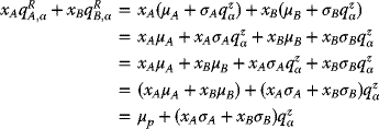
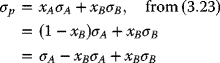
In this example, the return on the portfolio, Rp, over the following month is a random variable, given by
that is, a weighted average or linear combination of the random variables RA and RB. Moreover, as both RA and RB are assumed to be normally distributed, it follows from (3.23) that Rp is also normally distributed. Moreover, using the properties of linear combinations of random variables, (3.23) may be used to determine the mean and variance of the distribution of Rp, that is, the return of the entire portfolio.
Probable Expected Return and Variance of the Portfolio
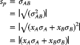
Again, according to (3.23), the mean, variance, and standard deviation of the distribution of the return on the portfolio may be readily derived as follows:
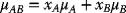
- The mean of the portfolio µp is given by
namely,
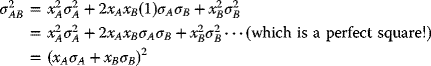
- The variance of the portfolio
 is given by
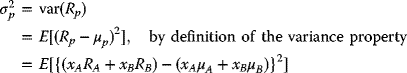
upon direct substitutions, respectively, from (3.23) and (3.24):

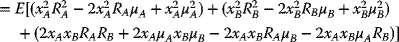
upon squaring the terms

upon expanding the multiplication of terms

upon removing all the parentheses
upon rearranging and recollecting terms

upon further rearranging and recollecting terms

upon further rearranging terms

upon further factoring terms

upon further factoring terms

upon further factoring the expression
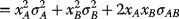
namely,
Finally,
- These relationships imply that
Remarks:
- Equation (3.25) shows that the variance of the portfolio is given as a weighted average of the variances of the individual component assets plus twice the product of the portfolio weights times the covariance between the component assets.
- Thus, if the portfolio weights are both positive, then a positive covariance will likely increase the portfolio variance since both returns tend to vary in the same direction. Likewise, a negative covariance may reduce the portfolio variance.
- Hence, assets with negatively correlated returns may be beneficial when building up a portfolio since the concomitant risk, as indicated by portfolio standard deviation, is reduced.
- Forming portfolios with positively correlated assets may reduce risk as long as the correlation is small.
Remark:
The following R-code* segment may be used for this computations:
- mu <- A*muA + B*muB

- var <- A*A*sigA*sigA + B*B*sigB*sigB + 2*A*B*sigAB)
*A comprehensive presentation of the R computer code is provided in Chapter 4.
Here, one may have recourse to using the R code to facilitate repetitive computations, in order to investigate results for other choices of xA, and hence xB.
Thus, for
the following R code segment would undertake the computation. The results follow, together with some graphic presentations of the results.
In the R domain:
>> muA <- 0.2> sigmasqA <- 0.05> muB <- 0.04> sigmasqB <- 0.01> sigA <- -0.2236> sigB <- -0.1000> sigAB <- -0.0038> rhoAB <- -0.17>> A <- c(1, 0.75, 0.50, 0.25, 0, 1.5, -0.5)> B <- c(0, 0.25, 0.50, 0.75, 1, -0.5, 1.5)> mu <- A*muA + B*muB> var <- A*A*sigA*sigA + B*B*sigB*sigB + 2*A*B*sigAB>> mu # Outputting:[1] 0.20 0.16 0.12 0.08 0.04 0.28 -0.04>> var # Outputting:[1] 0.04999696 0.02732329 0.01309924 0.00732481[2] 0.01000000 0.12069316 0.04069924>> plot(A, mu) # Outputting: Figure 3.2> plot(A, var) # Outputting: Figure 3.3>
Figure 3.3 var<- A*A*sigA*sigA + B*B*sigB*sigB + 2*A*B*sigAB.
Representing:
Representing:
Remarks:
- The variance of the portfolio is a weighted average of the variance of the individual assets plus twice the product of the portfolio weights times the covariance between the assets.
- If the portfolio weights are both positive, then a positive covariance will tend to increase the portfolio variance, because both returns tend to move in the same direction; likewise, a negative covariance will tend to reduce the portfolio variance.
- Hence, choosing assets with negatively correlated returns may be beneficial when forming portfolios because risk, as measured by portfolio standard deviation, is reduced.
- Note also that what forming portfolios with positively correlated assets can also reduce risk as long as the correlation is not too large.
In the R domain:
>> muA <- 0.2> sigmasqA <- 0.05> muB <- 0.04> sigmasqB <- 0.01> sigA <- -0.2236> sigB <- -0.1000> sigAB <- -0.0038> rhoAB <- -0.17>> A <- c(1, 0.75, 0.50, 0.25, 0, 1.5, -0.5)> B <- c(0, 0.25, 0.50, 0.75, 1, -0.5, 1.5)> mu <- A*muA + B*muB> var <- A*A*sigA*sigA + B*B*sigB*sigB + 2*A*B*sigAB> sigma <- sqrt(var)>> mu[1] 0.20 0.16 0.12 0.08 0.04 0.28 -0.04>> sigma[1] 0.2236000 0.1652976 0.1144519 0.0855851[5] 0.1000000 0.3474092 0.2017405>> plot(A, sigma) # Outputting: Figure 3.4> RER <- mu/sigma> RER[1] 0.8944544 0.9679513 1.0484753 0.9347421[5] 0.4000000 0.8059660 -0.1982745>> plot(A, RER) # Outputting: Figure 3.5
Figure 3.4 plot(A, sigma).

Figure 3.5 plot(A, RER).
3.2.3.2 Evaluating a Portfolio
Consider an initial investment I0 in a portfolio of assets A and B, for which
- the return is to be given by (3.23) ,
- the expected return is to be given by (3.24) , and
- the variance is to be given by (3.25) .
These relationships show that
Now, for α∈(0, 1), the 100α% portfolio value-at-risk is
where ![]() is the α quantile of the distribution of Rp and is given by
is the α quantile of the distribution of Rp and is given by
where ![]() is the α quantile of the standard normal distribution. If Rp is a continuously compounded return, then the implied simple return quantile is
is the α quantile of the standard normal distribution. If Rp is a continuously compounded return, then the implied simple return quantile is ![]() .
.
Relationship between the Portfolio VaR and the Individual Asset VaR
In general, the Portfolio VaR is not the weighted average of the Individual Asset VaRs. They may be seen in the following counterexample: Consider the portfolio weighted average of the individual asset return quantiles for a two-asset system (A, B) for which the weighted average of the asset return quantiles may be expressed as
Remark:
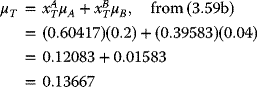
The weighted asset quantile (3.30) is not equal to the portfolio quantile (3.29) unless σp = ρAB = 1. Hence, weighted asset VaR, in general, is not equal to portfolio VaR because the quantile (3.30) ignores the correlation between RA and RB.
| µA | µB | σA | σB | σAB | ρAB | ||
| 0.2 | 0.05 | 0.04 | 0.01 | 0.2236 | 0.1000 | −0.0038 | −0.17 |
Remark: Note that
and
namely,
because
3.2.4 Management of Portfolios Consisting of Two Risky Assets
In the management of portfolios consisting of two risky assets, the approach may begin by constructing portfolios that are mean-variance efficient, using the following distribution of asset returns and the investors' behavior:
| 1. All returns are |
|
This implies that means, variances, and covariances of returns are constant over the investment horizon and completely characterize the joint distribution of returns.
- Investors know the values of asset return means, variances, and covariances.
- Investors are only concerned about the portfolio expected return and portfolio variance. Investors prefer portfolios with high expected return but not portfolios with high return variance.
With the above assumptions, it is possible to characterize the set of efficient portfolios, that is, those portfolios that have the highest expected return for a given level of risk as measured by portfolio variance. These portfolios are the investors' most likely choice.
For a numerical example of the management of portfolios consisting of two risky assets, use the data set in Table 3.2.
3.2.4.1 The Global Minimum-Variance Portfolio
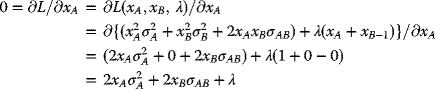
Using elementary calculus, finding the global minimum-variance portfolio is a simple exercise in calculus. This constrained optimization may be defined as
This is a constrained optimization problem and may be solved in the following two ways:
First Method: The method of substitution—using the constraint relationship to substitute one of the two variables (xA, xB) to transform the constrained optimization problem (in two variables) into an unconstrained optimization problem in only one variable. Thus, substituting, from xA + xB = 1, by inserting xB = 1 − xA into the formula for ![]() reduces the optimization problem to
reduces the optimization problem to
The condition for a local stationary point in the expression in (3.36) is that
The differentiation may be achieved using the chain rule:
Using (3.37), one obtains ![]() given by
given by
namely,
or
or
or
namely,
and
Second Method: The Method of Auxiliary Lagrange Multipliers λ—
| First, one puts the constraint: | xA + xB = 1 into a homogeneous form, |
| and writing: | F1 = xA + xB −1 = 0 |
| as well as: |
The Lagrangian Multiplier Function L is formed by adding to F2 the homogeneous constraint F1, multiplied by an auxiliary variable λ, the Lagrangian Multiplier, to give
Next, (3.39) is minimized, with respect to xA, xB, and λ, leading to three auxiliary conditions:
With the Lagrangian Multiplier Function L given by (3.39), one has


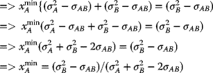
Combining (3.41a) and (3.41b), one obtains
namely,
namely,
namely,
namely,
namely,
or,
Finally, to obtain the required values ![]() , one may incorporate the third Lagrangian Multiplier condition (3.41c), namely, combining (3.42) and (3.41c):
, one may incorporate the third Lagrangian Multiplier condition (3.41c), namely, combining (3.42) and (3.41c):
Combining (3.43a) and (3.43b):


which is, of course, the same as (3.38a):
Finally,
which is, of course (again) (3.38b).
Remarks:
- In the Method of Auxiliary Lagrange Multipliers, the Lagrangian Multiplier Function, λ, is introduced at the beginning. And, after λ facilitated in solving the problem, in a rather elegant but indirect way, it is no longer required in further analysis!
- In the mathematics of optimization, the Method of Lagrange.
Langrangian Multipliers (named after the French mathematician Joseph Lagrange, 1811) are used as a methodology for locating the minima and the maxima of a function subject to a set of equality constraints. For instance, in Figure 3.7, consider the following optimization problem:
“To maximize f(x, y), subject to the constraint g(x, y) = 0.”
Figure 3.7 Method of Lagrange Multipliers: Finding x and y to maximize (or minimize), subject to a constraint (in red): g(x, y) = constant.
It is understood that both f and g have continuous first partial derivatives.
The Method of Lagrangian Multipliers
Introduce a new variable λ, called a Lagrange Multiplier and study the Lagrange Function (or the Lagrangian) defined by
where the λ term may be either added or subtracted. If f(x0, y0) is a maximum of f(x, y) for the original constrained problem, then there exists λ0 such that (x0, y0, λ0) is a stationary point for the Lagrange function (stationary points are those points where the partial derivatives of L are zero). However, not all stationary points yield a solution of the original problem. Thus, the method of Lagrange multipliers yields a necessary condition for optimality in constrained problems. Sufficient conditions for a minimum or maximum also exist (Figure 3.8).
Figure 3.8 Contour Map of Figure 3.7. The red line represents the constraint g(x, y) = c. The blue lines are contours of f(x, y). The solution is the point where the red line tangentially touches a blue contour. (Since d1 > d2, the solution is a maximization of the function f(x, y). (Both ordinates and abscissae are arbitrary.)
Suggested Exercise for Computation Using R:
As an exercise, write a program in R to undertake all the computations.
3.2.4.2 Effects of Portfolio Variance on Investment Possibilities
For a portfolio of any two assets, A and B, the correlation between A and B may strongly affect the investment possibilities of the portfolio. Thus,
- If ρAB is close to 1, then the investment set approaches a linear relationship such that the return is close to a straight line connecting the portfolio with all the funds invested in asset B, namely, (xA, xB) = (0, 1), to the portfolio with all the funds placed in asset A only, that is, (xA, xB) = (1, 0).
- In a plot of µp (as the ordinate) versus σp (as the abscissa) (see Figure 1.2), as ρAB approaches 0, the set bows toward the µp-axis, and the power of diversification starts to make its presence felt! If ρAB = −1, the set will actually tangentially touch the µp-axis. This implies that the assets A and B will be perfectly negatively correlated, and there exists a portfolio of A and B that has positively expected return but zero variance! And to determine the portfolio with
 when ρAB = −1, one may use (3.44a) and (3.44b), and the condition that(3.27)
to give
Since ρAB = −1
(3.45)
Now, from (3.44),
(3.44a)
And using (3.44b),
(3.44b)
3.2.4.3 Introduction to Portfolio Optimization
For the efficient set of portfolios as described in Figure 3.6, the critical question will be
“Which portfolio should an investor choose? And why?”
Of the efficient portfolios, investors will select the one that closely supports their risk preferences. In general, risk-averse investors will prefer a portfolio that has low risk, namely, low volatility, and will prefer a portfolio close to the global minimum-variance portfolio.
On the other hand, risk-tolerant investors will ignore volatility and seek portfolios with high expected returns. These investors will choose portfolios with large amounts of asset A that may involve short-selling asset B.
3.2.5 Attractive Portfolios with Risk-Free Assets
In Section 3.1.4, an efficient set of portfolios in the absence of a risk-free asset was constructed. Now consider what happens when a risk-free asset is being introduced.
A risk-free asset is equivalent to default-free pure discount bond that matures at the end of the assumed investment period. The risk-free rate rf, may be represented by the nominal return on a low-risk bond. For example, if the investment period is 1 month, then the risk-free asset is a 30-day U.S. Treasury bill (T-bill), and the risk-free rate is the nominal rate of return on the T-bill. (The “default-free” assumption of U.S. national debt has been questioned owing to the possible, and probable, inability of the U.S. Congress to address the long-term debt problems of the U.S. government.)
If the portfolio holding of the risk-free assets is positive, then it is equivalent to “lending money” at the risk-free rate. If the portfolio holding is negative, at “risk-free” rates, then one is “borrowing” money that is risk-free!
3.2.5.1 An Attractive Portfolio with a Risk-Free Asset
Consider an arbitrary portfolio with asset B, one may examine the consequences if one should introduce a risk-free asset (say, a T-Bill) into this portfolio.
Now the risk-free rate is constant (fixed) over the investment portfolio that has the following properties:
Then, within this portfolio,
- let the proportion of the investment in asset B = xB,
- then the proportion of the investment in T-Bills = (1 − xB)and hence the return of this portfolio is
Rp = Return owing to the asset B + return owing to the risk-free T-Bills = RB xB.
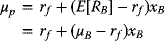
Hence, the portfolio return is given by
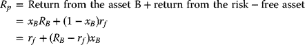
The term (RB − rf) is the Excess Return over the T-Bills return on asset B.
Hence, the Expected Return of the portfolio is
In (3.47), the factor (µB − rf) is the Expected Excess Return or Risk Premium on asset B.
Remarks:
- The risk premium is generally positive for risky assets, showing that investors will expect a higher return on the risky assets than the safe assets. This “risk premium” on the portfolio may be expressed in terms of the risk premium on asset B as follows, using (3.47):
(3.47)
 (3.48)
- Thus, the more one invests in asset B, the higher the risk premium on the portfolio.
- Since the risk-free rate is constant, the portfolio variance depends only on the variability of asset B, and is given by
(3.49)

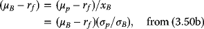
- Hence, the portfolio standard deviation is proportional to the standard deviation on asset B:
(3.50a)

which may be solved for xB:
- The Capital Allocation Line (CAL)—Combining (3.47) and (3.50b), one obtains the set of Efficient Portfolios:
(3.47)
 (3.48)
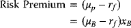
or
Hence,
which is a straight line in the (σp,µp)-space, with slope {(µB − rf)/σB}, and ordinate intercept rf.
This is the Capital Allocation Line (CAL)—see Section 3.1.1.7.
The slope of this line is the Sharpe Ratio (SR)—see Section 3.1.1.6. It is a measure of the risk premium on the asset per unit risk—as measured by the standard deviation of the asset.
- Characteristics of a two-asset portfolio with one asset taking short positions to appreciate the economic characteristics of a two-asset portfolio; one may consider the effects of combining two assets to form a portfolio. One can extend the analysis to cases in which short positions may be taken.
First, assume that one may either go long on the risk-free asset lend) or take a short position in it borrow) at the same interest rate, e1.
Let xA and xB be the proportions invested in assets A and B, respectively, and
let eA and eB be their respective returns.
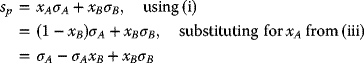
Then, the Expected Return of the whole portfolio, ep, will be given by
and since
namely,
(3.52) may be written as
namely,
The variance of the portfolio, varp, will be a function of
- the proportions, xA and xB, invested in these assets,
- their return variances: varA and varB, and
- the covariance between their returns: covarA–B:
Upon substituting (1 − xB) for xA to derive an expression relating the variance of the portfolio to the amount invested in asset B:
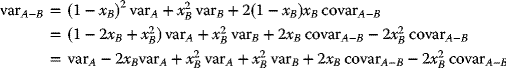
namely,
and the standard deviation of return, SDR, is the square root of this variance:
For any two given assets in a portfolio, and without loss of generality, one may assume that Asset 1 has less risk and, concomitantly, smaller expected return.
Now, consider the risk-return trade-offs associated with different combinations of the two assets. Also, consider the shape of the curves for mean-variance and mean-standard deviation plots that result as more investment is added to the risky asset, namely, as x2 (for the risky asset) is increased and x1 (for the risk-free asset) is decreased.
3.2.5.1.1 Investments with One Risk-Free Asset and One Risky Asset
When the investment consists only asset A and a risk-free asset (T-Bills), the Sharpe Ratio, SRA (viz., the excess return of an asset over the return of a risk-free asset divided by the variability or standard deviation of returns, see Section 3.1.1.6) is given by

On the other hand, when the investment consists only asset B and T-Bills, the Sharpe Ratio, SRB, is
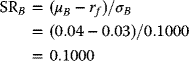
Here the data are taken from Table 3.2, and the risk-free rate, rf = 0.03, is the nominal return on the bond. Thus, for example, if the investment horizon is 1 month, then the risk-free asset is a “30-day U.S. Treasury Bill (T-Bill), and the risk-free rate rf is the nominal rate of return on the T-Bill.
Remarks:
- The expected return-risk trade-off for these portfolios are linear.
Figure 3.9 plots the locus of mean-standard deviation combinations for values.
If xA and xB are the proportions invested in assets A and B, respectively, and µA and µB are their respective expected returns, then the expected return of the portfolio of these two assets, µp, will be given by
Since

hence,

for xB between 0 and 1 when xA = 6, µB = 10, σA = 0, σB = 15, and covarA–B = 0.
In this case, as in every case involving a riskless and a risky asset, the relationship is linear. This is easily seen. Recall that ep is always linear in xB as shown earlier. If asset A is risk-free, sp (= xA σA + xB σB) will also be linear in xB, since both
 and covarA–B will equal zero. In such a case,
where |(xB)| denotes the absolute value of xB.
This result may be applied to cases where it is possible to take short positions. First, assume one can either go long on the risk-free asset (lend) or take a short position in it (borrow) at the same interest rate (eA). The above equations may then be applied. Figure 3.9 shows the results obtained by using leverage in this way. Thus, the point marked 1.5 is associated with xB = 1.5 and xA = −0.5. It shows that by “leveraging up” an investment in asset B by 50%, one may obtain a probability distribution of return on initial capital with an expected value of 12% and a standard deviation of 22.5%. The other points in the figure correspond to the indicated values of xB. Those above the original point involve borrowing (xA < 0) while those below it involve lending (xA > 0).
- The portfolios that are combinations of asset A and T-Bills have Expected Returns uniformly higher than the portfolios that are combinations of asset B and T-Bills. This result due to the Sharpe Ratio of asset A, 0.7603, is higher than the Sharpe Ratio of Asset B, 0.1000.
- The portfolios of asset A and T-Bills are more efficient relative to the portfolios of asset B and T- Bills.
- The Sharpe Ratio may be used as an index for ranking the return efficiencies of individual assets: Assets with higher Sharpe Ratios have superior risk-returns than assets with lower Sharpe Ratios. Thus, in financial engineering, analysts do rank assets on the basis of their Sharpe Ratios.
- For an investment portfolio consisting of a risky asset A and a risk-free asset (such as T-Bills), one may assume that the risk-free rate is constant (viz., fixed) over the investment period during which it has the following special properties: for the risk-free asset, it is assumed that
(3.56b)
 (3.56c)

Figure 3.9 Locus of mean standard deviations.
If xA denote the share of investment in asset A and xf denote the share of investment in the T-Bill portion of the portfolio, then
For this investment, the portfolio return, Rp, is given by

namely,
Remarks:
- The quantity (µA – rf), in (3.55), is the Expected Excess Return, or Risk Premium on asset A (over and above a risk-free asset). For risky assets, the Expected Excess Return is typically positive. That is, investors will expect a higher return on more risky investments.
- The Expected Excess on the portfolio may be expressed in terms of Expected Excess on the risky asset A as follows:
Equation (3.59) shows that for this category of investment portfolio, the greater the proportion of risky asset A invested, the higher the Expected Excess.
- Since the risk-free return rate is constant, the variance of the whole portfolio will depend only on the variability of the risky asset A, and is given by
Hence, the portfolio standard deviation σp is proportional to the standard deviation of asset A:
from which one may solve for xA:
- The feasibility and efficiency of the portfolio is given by the follow relationship: From (3.59):

and from (3.60c):
which is a straight line in the (µp, σp) space with slope {(µA − rf)/σA} and intercept rf.
The straight line (3.61) is the Capital Allocation Line (CAL) and the slope of CAL is called the Sharpe Ratio (SR) (formerly the Reward-to-Variability Ratio). It measures the ratio of the Expected Value of a zero-investment strategy to the Standard Deviation of that strategy. A special case of this approach involves a zero-investment strategy where funds are borrowed at a fixed rate of interest and invested in a risky asset!
Figure 3.10 plots the locus of mean-standard deviation combinations for values of xB between 0 and 1 when µA = 6, µB = 10, σA = 0, σB = 15 and covarA–B = 0.
As shown earlier,
- ep (= xAµA + xBµB) is always linear in xB, and
- If asset A is risk-free, sp (= xA σA + xB σB) will also be linear in xB, since both
 and covarA–B will equal zero. In such a case,

- If an investor short the risky asset (xB < 0) and invest the proceeds obtained from the short sale in the risk-free asset A, the standard equations apply. However, note that the variance will be positive, as will the standard deviation, since a negative number (xB) squared is always positive. Figure 3.11 shows the effects of negative xB values.
Figure 3.10 Effects of shorting the risky asset B.
Figure 3.11 A two-asset portfolio: 1 risk-free and 1 risky.
3.2.5.1.2 Investments with One Risk-Free Asset and Two Risky Assets
Next consider a portfolio of two risky assets, A and B, and some T-Bills. In this case, the efficient set will still be a straight line in the (µp, σp) space with intercept rj. The slope of the efficient set, namely, the maximum Sharpe Ratio, is such that it is tangential to the efficient set constructed just using the two risky assets A and B.
Remarks:
- If one invests only in asset A and T-Bills, then this gives a Sharpe Ratio of

and the Capital Allocation Line (CAL) will intersect the efficiency parabola (say, at point A). Thus, this is certainly not the efficient set of portfolios.
- On the other hand, if one invests only in asset B and T-Bills, then this gives a Sharpe Ratio of

and the Capital Allocation Line (CAL) will intersect the efficiency parabola (say, at point B). Again, this is certainly not the efficient set of portfolios.
- Indeed, one could do better if one invests some combination of assets A and B, together with some T-Bills. And clearly, the most efficient portfolio would be one such that the CAL is tangential to the parabola. This Tangency Portfolio will consist of assets A and B such that the CAL is just tangential to the parabola.
- And so the set of efficient portfolios will consist of such sets of assets A and B, together with some risk-free assets, such as T-Bills. These portfolios are Tangency Portfolio of assets A and B.
Remarks:
- If, during the process of allocation of assets, one takes short positions, and then the foregoing result can be extended to such cases as well.
- For example, if in one investment portfolio, one goes long on the risk-free asset (viz., “lend”), or chooses a short position instead (viz., “borrow”) at the same rate of interest, e1, then the above analysis may be applied.
- The results obtained from applying this leverage method is illustrated in Figure 3.10. Thus, the point labeled 1.5 is associated with

This shows that by the use of the leverage method applying to asset B by 50% (from xB = 1.0–1.5) in an investment, the investor may obtain a probability distribution of return on initial investment capital with
- an expected return value of 12% (as indicated in the ordinate of the “Expected return” axis), and
- a predicted standard deviation of 22.5% (as read on the abscissa of the “Standard Deviation” axis.
- In this figure, the other points correspond to the indicated values of xB = 0, 0.5, 1.0, and 2.0. Those above the original point (xB = 1.5) imply borrowing, namely, xA < 0 and xB > 1, and those points below the original point imply lending.
- Should an investor first short the risky asset, namely, xB < 0, and then invest the short sale proceeds in the risk-free asset xA, the analysis presented herein will still be applicable. However, in such cases, the variance and the standard deviation will be positive—since a negative number xB squared is positive. The effects of negative xB values is showed in Figure 3.11.
- In the world of business, it is a common practice that when moneys are borrowed, they usually come at a higher rate (say, 8%) than the rate at which they are being lent (say, 6%). This is being illustrated in Figure 3.14.
This plot shows the loci of the µAB–σAB combinations plotted as two lines, where
and

Figure 3.14 Effects between rate differences for “borrowed” and “lent” funds.
The first line is associated with the lower lending rate, and the second line is associated with the higher borrowing rate. Again, one may assume that the risky asset offers an Expected Return of 10% and a Risk of 15%. This efficient investment system is shown in Figure 3.14 in which the efficient frontier is represented by solid lines, and the options that are available if the investor could lend at 8% are shown in the broken line.
Moreover, the rates charged for borrowing may inverse with the loan amounts, so the locus of the σAB–µAB combinations may increase at a decreasing rate as the risk, σAB, increases beyond the amount for a full unlevered portfolio containing the risky asset: xB = 1. For such conditions, one may expect decreasing returns for taking risks!
To Combine Two Perfectly Positively Correlated Risky Assets
If the two returns are perfectly positively correlated, then σAB = 1, and (3.54) becomes
so that
Remarks:
- The notation |f(x)| denotes the absolute value of the enclosed expression f(x).
- Since neither σA nor σB is negative, when both xA and xB are nonnegative, the expression (xAσA + xBσB) in (3.55) will be nonnegative, and the absolute value of sp is understood implicitly. However, if one of the two x-values is sufficiently negative, then the absolute value of sp should be used explicitly.
- For long positions in the two assets, namely, xA, xB ≥ 0, consider the following combinations:
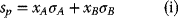

Since

By substituting for xA in (i), using (iii), one obtains from (i):
or
(3.56)
Similarly, by substituting for xA in (ii), using (iii), one obtains from (ii):
or
(3.57)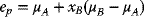
- All such relationships will lie on a straight line, which represents the two assets (see Figure 3.15).
- Extension of the values of xB to xB > 1 or xB < 0:
Consider the Minimum-Variance Portfolio, namely, the combination that results in the least possible risk. To achieve a variance of 0, one may seek the value of xB for which sp = 0. And using (3.56):

Solving for xB:,
and
Applying this result to the foregoing numerical example, it may be seen that a risk-free portfolio may be obtained by using (3.58a):
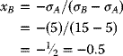
and (3.58b):
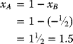
- This portfolio may be achieved by taking a short position in asset B equal to half of the total investment funds and investing this amount, together with the original amount of funds, in asset A. This action may need the pledging of some other collateral to form an adequate guarantee to the lender of asset B that the short position may be covered whenever required.
- The need to create a risk-free portfolio by choosing offsetting positions in two perfectly positively correlated assets results in creating a configuration similar to the case for a risk-free asset combining with a risky asset. The following steps show how this goal may be achieved:
Let the expected return on the zero-variance portfolio be
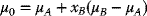
Hence, for the foregoing numerical examples, µA = 8, µB = 10, and xB = −0.5,
And the portfolio returns and risks may be obtained by considering any combinations of the risk-free asset A and either asset A or asset B. Either option provides the graph associated with a risk-free asset and a risky asset. This result is illustrated in Figure 3.16.
- In this case, as in every case involving a risk-free and a risky asset, the relationship is linear. This is easily seen. Recall that ep is always linear in xB, as shown earlier. If asset A is risk-free, sp will also be linear in xB, since both
 and covarA–B will equal zero. In such a case,

namely,

where |xB| denotes the absolute value of xB.For cases in which it is possible to take short positions, this result is applicable: First assume one may either go long (viz., to lend) with the risk-free asset A or take a short position in it (viz., to borrow) at the same rate of interest µA. Then the foregoing formulas may be applied directly: This case has been illustrated in Figure 3.10 and Example 3.8.
- Figure 3.17 shows the locus of mean standard deviation combinations for values of xB between 0 and 1, when


Figure 3.15 Two perfectly positively correlated risky assets: σAB = 1, Point 1: Asset A, for which µA = 8, σA = 5; Point 2: Asset B, for which µB = 10, σB = 15. 
Figure 3.16 Creating a risk-free portfolio: µ0 = 7, by choosing off-setting positions in two perfectly positively correlated assets: Point 1: Asset A, for which µA = 8, σA = 5; Point 2: Asset B, for which µB = 10, σB = 15.

Figure 3.17 Combining a risk-free asset and a risky asset when µA = 6, µB = 10, σA = 0, σB = 15, and covarA−B = 0.
Again, in this special case, as in cases involving a risk-free asset and a risky asset, the relationship is linear. This observation may be shown as follows:
Since
ep is linear in xB; and when asset A is risk-free, sp will also be linear in xB. Since
both ![]() and covarA–B will equal zero. Therefore,
and covarA–B will equal zero. Therefore,
and
where |xB| is the absolute value of xB.
Remark: It should not escape one's attention that when an investment involves short positions, and between ending asset and liability values, additional liquid capital must be pledged to cover these short positions, as well as possible liability values. Alternatively, a higher rate may have to be charged accordingly for all the short positions.
Remarks:
- The cases are coincidental at the endpoints (x1 = 1, x2 = 0) and (x1 = 0, x2 = 1).
- For all interior combinations, when the Correlation Coefficient ρAB < 1.0, risk is less than proportional to the risks of two assets; the greater the extent of risk reduction, the smaller the correlation coefficient:
- The yellow curve, r12 = 1.0, provides no risk reduction, only risk-averaging.
- The red curve, r12 = 0.5, provides some risk reduction.
- The green curve, r12 = 0, provides some more risk reduction.
- The blue curve, r12 = 0.5, provides even more.
Remarks:
- |f(xA, xB)| represents the absolute value of the expression enclosed.
- If both xA and xB are nonnegative, namely, zero or positive, then the expression (xAσA + xBσB) will be nonnegative, since neither σA nor σB is negative.
- If either xA or xB is sufficiently negative, the expression (xAσA + xBσB) may become negative, and the absolute value should apply.
- Risks: From the combinations of long positions in these two assets, namely,
and in any such combinations: σp = xAσA + xBσB, from (3.23),
namely,
(3.56)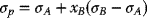
- Similarly, for returns, for such combinations:

namely,
(3.57)
- In Figure 3.20, the σ–µ plot represents the following system:

Both the risk and the return will be proportional to xB, such portfolios will be on a straight line—connecting the points representing the two assets, namely, point 1: (σA = 5, µA = 8), and point 2: (σB = 15, µB = 10).
Figure 3.20 A portfolio of two perfectly positively correlated risky assets.
Remarks:
- In Figure 3.21, the minimum-variance portfolio (in white) is a familiar and distinctive diagram—see Figures 3.9–3.12, 3.15, and 3.17—for portfolios that has one risk-free asset.
- Note that long positions in two perfectly negatively correlated assets are similar to the following:
- A long position in one of two perfectly positively correlated assets.
- A short position in the other asset.
- In many cases, asset correlations have values between −1 and +1.
- A general formula for the minimum-variance portfolio may be derived as follows: Starting with a reduced-form equation where the variance varp of a two-asset portfolio is being expressed as a function of xB, starting with
(3.54)
for the two-asset portfolio, assets A and B.
Differentiating both sides of (3.54), with respect to xB, namely, undertaking the ∂/∂xB operation on both sides of (3.54), the result is
(3.55)
To obtain a stationary point, one sets (3.55) to zero, and solve for the value of xB that will provide the minimum-variance portfolio, namely, solving for xB-min. The result is

from which
(3.56)
This minimum-variance portfolio may have a lower risk than either of the two-component assets, and may also have a higher return!
- Considering the point at which xB = 0, one has
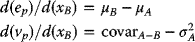
and
(3.57)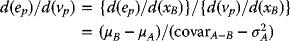
Assuming that µB > µA, if the slope d(ep)/d(vp) is to be negative, then (3.57) shows that
or
(3.58)
For example, if σA = 5, σB = 15, µB > µA, and σAB < 5/15, the minimum-variance portfolio will dominate asset A, resulting in both higher expected return and lower risk—a double bonus!
3.2.5.2 The Tangency Portfolio
Next, one may proceed to expand the foregoing analysis by considering portfolios consisting of asset A, asset B, and risk-free asset (say, T-Bills). For this case, the efficient set will also be given by (3.51):
namely, a straight line in the (µp, σp) space with intercept rf. For this efficient set, its slope is the maximum Sharpe Ratio, namely, it is tangential to the efficient set consisting of only the two risky assets: A and B.
Tangent Portfolios are portfolios of stocks and bonds designed for long-term investors. To find the Tangent Portfolios, one may start by asking how much one would be prepared to lose in a worst-case scenario without dropping out of the market: 20%? 25%? or 33%? Once the maximum loss level is chosen, the Tangent Portfolios will try to deliver a high rate of return for that level of risk.
There is a human temptation to invest on the basis of the BLASH (Buy-High-And-Sell-Low) route! Thus, most investors tend to take on large amounts of risk during good times (Buy High), and then sell out during bad times (Sell Low)—ruining their returns in the process. The Tangent Portfolios are designed to let the investor do well enough during both good and bad times to keep one in the markets throughout. This allows the investor reap the long-term benefits from investing in stocks and bonds with a simple, low-maintenance solution.
Figure 3.22, same as Figure 3.1, illustrates the Efficient Frontier. The hyperbola is sometimes referred to as the Markowitz Bullet, and is the efficient frontier if no risk-free asset is available. With a risk-free asset, the straight line is the efficient frontier.

Figure 3.22 The tangency portfolio (same as Figure 3.1).
Efficient Frontiers
Different combinations of assets may produce different levels of return. The Efficient Frontier represents the best of these combinations, that is, those that produce the maximum expected return for a given level of risk. The efficient frontier is the basis for modern portfolio theory.
Example of Efficient Frontiers
Markowitz, in 1952 (see Figure 3.23), published a formal portfolio selection model in The Journal of Finance. He continued to develop and publish research on the subject over the next 20 years, eventually winning the 1990 Nobel Memorial Prize in Economic Science for his work on the efficient frontier and other contributions to modern portfolio theory. According to Markowitz, for every point on the efficient frontier, there is at least one portfolio that can be constructed from all available investments that has the expected risk and return corresponding to that point. An example is given here: Notice that the efficient frontier allows investors to understand how an expected returns of a portfolio vary with the amount of risk taken.

Figure 3.23 The efficient frontier according to Markowitz (1952).
An important part of the efficient frontier is the relationship that the invested assets have with one another. Some assets' prices move in the same direction under similar circumstances, while others move in opposite directions. The more out of step that the assets in the portfolio are (i.e., the lower their covariance), the smaller the risk (standard deviation) of the portfolio that combines them. The efficient frontier is curved because there is a diminishing marginal return to risk. Each unit of risk added to a portfolio gains a smaller and smaller amount of return. When Markowitz introduced the efficient frontier, it was a seminal contribution to financial engineering science: One of its greatest contributions was its clear demonstration of the power of diversification.
Markowitz's theory relies on the claim that investors tend to choose, either purposely or inadvertently, portfolios that generate the largest possible returns with the least amount of risk. In other words, they seek out portfolios on the efficient frontier!
It should not be unaware that there is no one efficient frontier because individual investors as well as portfolio managers can and do edit the number and characteristics of the assets in the investing universe to conform to their own personal specific needs. For example, one individual investor may require the portfolio to have a minimum dividend yield, or another client may rule out investments in ideologically (e.g., politically, ethically, ethnically, or religiously) nonpreferred industries. Thus, only the remaining assets are included in the efficient frontier calculations.
Recent Historical Performance of the Stock Market
Maximum Losses: For all the rolling 12-month periods from 2010 going back to 1926:
- The Tangent 20 portfolio had a maximum 1 year inflation-adjusted loss of 20%
- The Tangent 25 portfolio had a maximum 1 year inflation-adjusted loss of 25%
- The Tangent 33 portfolio had a maximum 1 year inflation-adjusted loss of 33%
The period 1926–2010 includes the following extraordinary events:
- The stock market crash of 1929
- The Great Depression
- The World War II
- The Cold War
- Sputnik
- Assassination of a U.S. President
- Race riots
- The Vietnam War
- Inflation
- The stock market crash of 1987
- 9/11 (2001)
- Bubbles and collapse of the .com bubbles
- The panic of 2008
- and so on.
These estimates of losses form historical benchmarks of the bad times that the stock market might face!
The following table shows that the performance of various portfolios respond after correcting for inflation over rolling 12-month periods from 1926 to 2008, before adjusting for applicable taxes and other relevant expenses.
Remarks:
- The Tangent 20 portfolio delivered almost twice the average returns of a portfolio of Treasury Bills, with only slightly more risk of 1-year loss.
- The Tangent 33 portfolio delivered most of the returns of the U.S. stock market, with substantially less risk.
- These are hypothetical and historical notations for reference.
- There is no guarantee that these levels of risk or returns will be maintained in the future.
- Individual investment losses or gains may vary, depending on the levels of risk tolerance, investment objectives, and so on (Table 3.3).
Table 3.3 Estimated total stock market returns, 1926–2008.
| Portfolios | Average year | Worst year |
| U.S. Stocks | 7.9% | −65% |
| Tangent 33 | 7.6% | −33% |
| Tangent 25 | 6.0% | −25% |
| Tangent 20 | 4.6% | −20% |
| T-Bills | 2.4% | −16% |
3.2.5.3 Computing for Tangency Portfolios
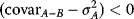
To estimate the Tangency Portfolios, one may begin by determining the values of xA and xB that maximize the Sharpe Ratio of the portfolio that is on the envelope of the parabola.
For a given set of two available assets A and B to formally solve for the Tangency Portfolio, the task consists of finding the values of xA and xB that maximize the Sharpe Ratio (SR) of a portfolio that is on the envelope of the parabola: This calls for solving the following constrained maximization problem:
such that

This problem, as stated in (3.59a) and (3.59b), may be reduced to
for which the solutions are as follows:
A Numerical Example for the Tangency Portfolio for the Sample Data
For the example data in Table 3.2 and using (3.60a) and (3.60b), one obtains
and
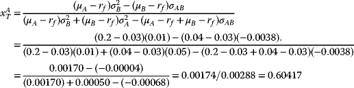
The expected return, variance, and standard deviation on this tangency portfolio are
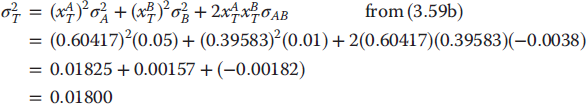

Cleary, if repeated computations are required, a simple R code may be used to undertake the numerical calculations involving (3.59) and (3.60)
3.2.6 The Mutual Fund Separation Theorem
Until this point, it has been shown that the efficient portfolios are combinations of two classes of assets:
- Tangency portfolios
- Risk-free assets, such as T-Bill
Hence, applying (3.56) and (3.57b):
one may write the expected return and standard deviation of any efficient portfolios:
where
- xT represents the fraction of investments in the tangency portfolio,
- (1 − xT) represents the fraction of wealth invested in risk-free assets (e.g., T-Bills), and
- µT and σT represent, respectively, the expected return and standard deviation of the tangency portfolio.
This result is called the Mutual Fund Separation Theorem.
Remarks:
- The Tangency Portfolio may be considered as a mutual fund of two risky assets—in which the shares of the two risky assets are determined by the tangency portfolio weights:
 and
and  determined from (3.60a) and (3.60b), and the T-Bills may be considered as a mutual fund of risk-free assets.
 - The exact combination of the tangency portfolio and the T-Bills will be dependent on the risk preference of the investor: If the investor is highly risk-adverse, then this investor may choose a portfolio with low volatility, namely, a portfolio with very small weight in the tangency portfolio together with a very large weight in the T-Bills! Clearly, this option will produce a portfolio with an expected return close to the risk-free rate, and a variance that is nearly zero! On the other hand, if the investor can tolerate a large amount risk, then the preferred portfolio will have high expected return regardless of the volatility.
This portfolio may consist of borrowing at the risk-free rate (known as “leveraging”) and investing the proceeds in the tangency portfolio to achieve an overall high expected returns.
3.2.7 Analyses and Interpretation of Efficient Portfolios
For a given risk level, efficient portfolios have high expected returns—as measured by portfolio standard deviations. Thus, for those portfolios that yield expected returns above the T-Bill rates, the efficient portfolios may also be characterized as those that have minimum risks for a given target expected return—as measured by the portfolio standard deviation.
3.3 The Black–Litterman Model
With the foregoing discussions of the development of the study of asset allocation in terms of Markowitz's Modern Portfolio Theory of the mean-variance approach to asset allocation and portfolio optimization, this may well be the suitable point of departure to go from the Markowitz model on to the Black–Litterman model.
Asset allocation is the continuing decision facing an investor who must decide on the optimum allocation of the assets in the portfolio across a few (say up to 20) asset classes. For example, a globally invested mutual fund must select the proportions of the total investment for allocation to each major country or global financial region.
It is true that the Modern Portfolio Theory (the mean-variance approach of Markowitz) may provide a plausible solution to this problem once the expected returns and covariances of the assets are available. Thus, while Modern Portfolio Theory is an important theoretical approach, its application does encounter a serious problem: Although the covariances of a few assets may be adequately estimated, it is difficult to ascertain (with reasonable estimates) of the Expected Returns!
The Black–Litterman approach resolves this problem by the following:
- Not requiring the use of input estimates of expected return.
- Instead, it assumes that the initial expected returns are whatever is required so that the equilibrium asset allocation is equal to what one observes in the markets.
- The user is only required to state how one's assumptions about expected returns differ from the expected returns in the market, and to state one's degree of confidence in the alternative assumptions.
- From this, the Black–Litterman method computes the preferred Mean-Variance Efficient asset allocation.
In general, to overcome portfolio constraints—for example, when short sales are not allowed— the way to find the optimal portfolio is to use the Black–Litterman model to generate the expected returns for the assets, and then use a mean-variance optimization procedure to solve the resultant optimization problem.
Efficient Frontier
What It Is
Different combinations of securities produce different levels of return. The efficient frontier represents the best of these securities combinations—those that produce the maximum expected return for a given level of risk. The efficient frontier is the basis for modern portfolio theory.
How It Works (Example)
In 1952, Harry Markowitz published a formal portfolio selection model in The Journal of Finance. He continued to develop and publish research on the subject over the next 20 years, eventually winning the 1990 Nobel Prize in Economic Science for his work on the efficient frontier and other contributions to modern portfolio theory.
According to Markowitz, see Figure 3.26, for every point on the efficient frontier, there is at least one portfolio that can be constructed from all available investments that have the expected risk and return corresponding to that point.

Figure 3.26 Efficient frontier.
An example appears below. Note how the efficient frontier allows investors to understand how a portfolio's expected returns vary with the amount of risk taken.
To have relationship securities with each other is an important part of the efficient frontier. Some securities' prices move in the same direction under similar circumstances, while others move in opposite directions. The more the out of sync securities in the portfolio (i.e., the lower their covariance), the smaller the risk (standard deviation) of the portfolio that combines them. The efficient frontier is curved because there is a diminishing marginal return to risk. Each unit of risk added to a portfolio gains a smaller and smaller amount of return.
Why It Matters
When Markowitz introduced the efficient frontier, it was groundbreaking in many respects. One of its largest contributions was its clear demonstration of the power of diversification.
Markowitz's theory relies on the claim that investors tend to choose, either purposefully or inadvertently, portfolios that generate the largest possible returns with the least amount of risk. In other words, they seek out portfolios on the efficient frontier.
However, there is no one efficient frontier because portfolio managers and investors can edit the number and characteristics of the securities in the investing universe to conform to their specific needs. For example, a client may require the portfolio to have a minimum dividend yield, or the client may rule out investments in ethically or politically undesirable industries. Only the remaining securities are included in the efficient frontier calculations.
3.4 The Black–Scholes Option Pricing Model
| x1 = xA= x2 = xB e1 = µA e2 = µB ep = x1*e1 + x2*e2 = xA µA + xB µB r12 = σAB = var1-2 s1 = σA s2 = σB sp = x1*s1 + x2*s2 = xA σA + xB σB v1 = varA = σ2A v2 = varB = σ2B vp = var1-2 = σ2AB c12 = covarA-Bhttps://web.stanford.edu/∼wfsharpe/mia/rr/mia_rr5.htm (6) p. 22 of http://faculty.washington.edu/ezivot/econ424/introductionPortfolioTheory.pdf |
| Package: | Sim.DiffProc |
3.4.1 Keep on Modeling!
Modern Portfolio Theory (MPT) has also been criticized for its assumptions that returns follow a Gaussian distribution. In the 1960s, several workers had shown the inadequacy of this assumption and proposed the use of stable distributions as well strategies for deriving optimal portfolios in such settings. Some notable suggestions were as follows:
- Since the introduction of MPT in 1952, a number of attempts have been advanced with the sole purpose to improve this model by including more Realistic assumptions. These include the following:
- The Post-Modern Portfolio Theory (PMPT), which extends MPT by using nonnormally distributed asymmetric measures of risk. This approach has been found useful in some, but not all, cases.
- In the 1970s, Conroy, using concepts from MPT, applied the economic analysis in the field of regional science, modeled the labor force in the economy by a portfolio–theoretic approach to analyze growth and variability in the labor force. This work led to the analysis of the relationship between volatility and economic growth.
Thus, while MPT is a useful introductory framework, more work is needed to render it useful and reliable in practice. Since the introduction of MPT in 1952, notable attempts made to improve the model, especially by using more realistic assumptions, Post-modern Portfolio Theory extends MPT by adopting nonnormally distributed, asymmetric measures of risk—This adjustment helps with some of these problems, but not all!
- Other Formulations
In the 1970s, concepts from MPT found their way into the field of Regional Science. In a series of seminal works, Conroy modeled the labor force in the economy using portfolio–theoretic methods to examine growth and variability in the labor force. This was followed by an extensive study on the relationship between economic growth and volatility.
Recently, modern portfolio theory has been applied to the following:
- Social Psychology—For Modeling the Self-Concept: When the self attributes comprising the self-concept constitute a well-diversified portfolio, then psychological outcomes at the level of the individual such as mood and self-esteem should be more stable than when the self-concept is undiversified. This prediction has been confirmed in studies involving human subjects.
- Information Science: For modeling the uncertainty and correlation between documents in information retrieval. Given an open question, one may maximize the relevance of a ranked list of documents and at the same time minimize the overall uncertainty of the ranked list.
- Other Nonfinancial Assets: MPT has also been applied to portfolios of assets besides financial instruments. When MPT is applied to nonfinancial portfolios, the characteristics among the different types of portfolios should be considered, for example:
- The assets in financial portfolios are, for practical purposes, continuously divisible while portfolios of projects are “lumpy.” Thus, for example, while one may compute that the optimal portfolio position for four stocks is, say, 45, 26, 20, and 9%, the optimal position for a project portfolio may not allow us to simply change the amount spent on a project. Projects may be all or nothing or, at least, have logical units that cannot be separated. Thus, a portfolio optimization method would have to take the discrete nature of projects into account.
- Assets of financial portfolios are liquid: They may be assessed or reassessed at any point in time. However, opportunities for starting new projects may be limited and may occur in limited time windows. Projects that have already been initiated may not be abandoned without the loss of the sunk costs (i.e., there may be little or no salvage value of a partly complete project).
Neither of these factors necessarily eliminate the possibility of using MPT for such portfolios. However, they require the need to run the optimization with an additional set of mathematically expressed constraints that would not normally apply to financial portfolios. Furthermore, some of the simplest elements of MPT are applicable to virtually any kind of portfolio. The concept of ascertaining the risk tolerance of an investor by documenting the quantity of risk that is acceptable for a given return may be applied to a variety of decision analysis problems. MPT uses historical variance as a measure of risk, but portfolios of assets like major projects generally do not have a well-defined “historical variance.” In such cases, the MPT investment boundary may be expressed in more general terms like “the chance of an ROI (Return-On-Investment) less than cost of capital,” or “the chance of losing more than half of the investment.” Thus, when the risk is expressed in terms of uncertainty about forecasts, and possible losses, then the concept of MPT may be transferable to various types of investment.
- Black–Litterman Model (BL), introduced in 1990, advanced that the optimization should be an extension of unconstrained Markowitz optimization that incorporates relative and absolute views on inputs of risks and returns. This will be fully discussed in Section 3.5.
3.5 The Black–Litterman Model
The goals of the Black–Litterman model were as follows:
- To create a systematic method of specifying a portfolio
- To incorporate the views of the analyst/portfolio manager views into the estimation of market parameters.
Let
be a set of random variables representing the returns of n assets. In the BL model, the joint distribution of A is taken to be multivariate normal,
that is,
The model then considers incorporating an analyst's views into the estimation of the market mean µ. If one considers
- µ to be a random variable that is itself normally distributed and that
- its dispersion is proportional to that of the market,
then
where π is some parameter that may be determined by the analyst by some established procedure—as will be seen in the remainder of this section: On this point, Black and Litterman proposed (based on equilibrium considerations) that this should be obtainable from the intercepts of the capital-assert pricing model.
Next, upon the consideration that the analyst has certain subjective views on the actual mean of the return for the holding period, this part of the BL model may allow the analyst to include personal views. BL suggested that such views should best be made as linear combinations, namely, portfolios, of the asset return variable mean µ:
- Each such personal view may be allocated a certain mean-and-error, (µi, ɛi), so that a typical view would take the form
where ![]() .
.
The standard deviations ![]() of each view may be assumed to control the confidence in each. Expressing these views in the form of a matrix, call the “pick” matrix, one obtains the “general” view specification:
of each view may be assumed to control the confidence in each. Expressing these views in the form of a matrix, call the “pick” matrix, one obtains the “general” view specification:
in which Ω is the diagonal matrix diag![]() . It may be shown, using Bayes' law, that the posterior distribution of the market mean conditional on these views is
. It may be shown, using Bayes' law, that the posterior distribution of the market mean conditional on these views is
where
One may then obtain the posterior distribution of the market by taking
which is independent of µ.
One may then obtain
and
The Canonical Black–Litterman Reference Model
The remainder of the Black–Litterman model is built on the reference model for returns. It assumes which variables are random, and which are not. It also defines which parameters are modeled, and which are not. Other reference models have been Alternative Reference Model or Beyond Black–Litterman, which do not have the same theoretical basis as the canonical one that was initially specified in Black and Litterman (1992).
Starting with normally distributed expected returns,
The fundamental objective of the Black–Litterman model is to model these expected returns, which are assumed to be normally distributed with mean µ and variance ∑. Note that one will need at least these values, the expected returns, and covariance matrix later as inputs into a portfolio selection model.
Define µ, the unknown mean return, as a random variable itself distributed as
π is the estimate of the mean and ∑π is the variance of the unknown mean, µ, about the estimate. Another way to view this linear relationship is shown in the following formula:
These prior returns are normally distributed around π with a disturbance value ɛ. Figure 3.27 shows the distribution of the actual mean about the estimated mean of 5% with a standard deviation of 2% (or a variance of 0.0004).

Figure 3.27 The estimated mean and the distribution of the actual mean about the estimated mean ɛ, which is normally distributed with mean 0 and variance ∑π and is assumed to be uncorrelated with µ.
Clearly, this is not a precise estimate from the width of the peak. One may complete the reference model by defining ∑r as the variance of the returns about the initial estimate π.
From (3.77) and the assumption above that ɛ and µ are not correlated, the formula for calculating ∑π is
(3.78) shows that the proper relationship between the variances is (∑r ≥ ∑, ∑π).
One may check the reference model at the boundary conditions to ensure that it is correct. In the absence of estimation error, that is, ɛ = 0, ∑r = ∑. As the estimate gets worse, if ∑π increases, then ∑r also increases.
For the Black–Litterman model expected return, the canonical reference model is
It should be emphasized that (3.79) is the canonical Black–Litterman reference model, and not (3.76).
Remarks:
- A common misconception about the Black–Litterman model is that (3.76) is the reference model, and also
- µ is a point estimate in the model.
Computing the Equilibrium Returns
The Black–Litterman model begins with a neutral equilibrium portfolio for the prior estimate of returns. The model relies on General Equilibrium theory, namely, that “if the aggregate portfolio is at equilibrium, then each sub-portfolio must also be at equilibrium.” It may be used with any utility function, making it very flexible. In fact, most practitioners use the Quadratic Utility function and assume a risk-free asset, and thus the equilibrium model simplifies to the Capital Asset Pricing Model (CAPM). In fact, the neutral portfolio in this case is the CAPM Market portfolio.
Some workers have used other utility functions, and others consider other measures of portfolio risk without applying the same theoretical basis. In order to preserve the symmetry of the model, the practitioner should use the same utility function to identify both the neutral portfolio and the portfolio selection area. Here the approach uses the Quadratic Utility function, CAPM, and unconstrained mean-variance because it is a well-understood model. Given these assumptions, the prior distribution for the Black–Litterman model is the estimated mean excess return from the CAPM market portfolio. The process of computing the CAPM equilibrium excess returns is straightforward. CAPM is based on the concept that there is a linear relationship between risk (as measured by standard deviation of returns) and return. Furthermore, it requires returns to be normally distributed. This model is of the form
where
- rf is the risk-free rate,
- rm is the excess return of the market portfolio,
- β is the a regression coefficient computed as β = ρ (σp/σm), and
- α is the residual or asset-specific excess return.
Under CAPM, any irregular risks associated with an asset is uncorrelated with that from other assets, and this issue may be reduced via diversification. And the investor may be rewarded for taking systematic risk measured by β, but is not compensated for taking irregular risks associated with α.
Under CAPM, all investors should hold the same risky CAPM market portfolio. Since all investors hold risky assets only in the market portfolio, at equilibrium their weights in the market portfolio will be determined by the market capitalization of the various assets. On the efficient frontier, the CAPM market portfolio has the maximum Sharpe Ratio of any portfolio. Here, the Sharpe Ratio is the excess return divided by the excess risk, or (r – rf)/σ.
The investor may also invest in a risk-free asset. This risk-free asset has essentially a fixed positive return for the time period over which the investor is concerned. It is generally similar to the sovereign bond yield curve for the investors' local currency—such as the U.S. Government Treasury Bills. Depending on how the asset allocation decision will be framed, this risk-free asset can range from a 4-week Treasury Bill (1-month horizon) to a 20-year inflation protected bond.
The CAPM market portfolio contains all investable assets that makes it difficult to specify. Since the system is in equilibrium, all submarkets must also be in equilibrium and any submarket chosen is part of the global equilibrium. While this permits one to reverse optimize the excess returns from the market capitalization and the covariance matrix, forward optimization from this point to identify the investors optimal portfolio within CAPM is difficult since one does not have information for the entire market portfolio. In general, this is not actually the question investors are asking, usually most investors select an investable universe and search for the optimal asset allocation within the universe: Thus, the theoretical problem with the market portfolio may be initially ignored.
The Capital Market Line
The Capital Market Line is a line through the risk-free rate and the CAPM market portfolio. The Two Fund Separation Theorem, closely related to the CAPM, states that all investors should hold portfolios on the Capital Market Line. Any portfolio on the Capital Market Line dominates all portfolios on the Efficient Frontier, the CAPM market portfolio being the only point on the Efficient Frontier and on the Capital Market Line. Depending on one's risk aversion, an investor will hold arbitrary fractions of their investment in the risk-free asset and/or the CAPM market portfolio. Figure 3.20 shows the relationship between the Efficient Frontier and the Capital Market Line.
To start the market portfolio, one may choose to start with a set of weights that are all greater than zero and naturally sum to 1. The market portfolio only includes risky assets, because by definition investors are rewarded only for taking on systematic risk. Thus, in the CAPM, the risk-free assets with β = 0 will not be in the market portfolio. At a later stage, one will see that the Bayesian investor may invest in the risk-free asset based on their confidence in their return estimates. The problem may be constrained by asserting that the covariance matrix of the returns, ∑, is known. In fact, this covariance matrix may be estimated from historical return data. It is often calculated from higher frequency data and then scaled up to the time frame required for the asset allocation problem.
By calculating it from actual historical data, one may ensure that the covariance matrix is positive definite. Without basing the estimation process on actual data, there may be significant issues involved in ensuring the covariance matrix is positive definite. One may apply shrinkage or random matrix theory filters to the covariance matrix in an effort to make it robust.
In this approach, one may use a common notation, similar to that used in He and Litterman (1999). Note that this notation is unusually different.
First, one derives the equations for ‘reverse optimization’ starting from the quadratic utility function:
where
- U is the investors' utility, the objective function during Mean-Variance Optimization,
- w is the vector of weights invested in each asset,
- ∏ is the vector of equilibrium excess returns for each asset,
- δ is the risk aversion parameter, and
- ∑ is the covariance matrix of the excess returns for the assets.
Now, U, being a convex function, will have a single global maxima. If one maximizes the utility with no constraints, then there is a closed-form solution. The exact solution may be found by taking the first derivative of (3.81) with respect to the weight w and setting it to zero:
Solving (3.82) for ∏ (the vector of excess returns) yields:
In order to use (3.83) to solve for the CAPM market portfolio, one needs to have a value for δ, the risk aversion coefficient of the market. One way to find δ is by multiplying both sides of (3.83) by wT and replacing vector terms with scalar terms:
Here the expression at equilibrium is that the excess return to the portfolio is equal to the risk aversion parameter multiplied by the variance of the portfolio. From (3.84),
where
- r is the total return on the market portfolio (r = wT∏ + rf),
- rf is the risk-free rate, and
- σ2 is the variance of the market portfolio (σ2 = wT∑w)
Many specify the value of δ used. For global fixed income, some use a Sharpe Ratio of 1.0. Black and Litterman (1992) use a Sharpe Ratio closer to 0.5. Given the Sharpe Ratio (SR), one rewrite (3.85) for δ in terms of SR as
One may now calibrate the returns in terms of formulas (3.85) or (3.86). As part of the analysis, one should arrive at the terms on the right-hand side of which formula one chooses to use. For (3.85), this is r, rf, and σ2 in order to calculate a value for δ. For (3.86), this is the Sharpe Ratio SR and σ.
To use formula (3.85), one needs to have an implied return for the market portfolio that may be more difficult to estimate than the SR of the market portfolio.
With this value of δ, substitute the values for w, δ, and ∑ into (3.83) to obtain the set of equilibrium asset returns. Equation (3.83) is therefore the closed-form solution to the reverse optimization problem for calculating asset returns given an optimal mean-variance portfolio in the absence of constraints. One may rearrange Equation (3.83) to yield the formula for the closed-form computation of the optimal portfolio weights in the absence of constraints.
Herold (2005) provides insights into how implied returns can be calculated in the presence of simple equality constraints such as the budget or full investment (∑w = 1) constraint. It was shown how errors may be introduced during a reverse optimization process if constraints are assumed to be nonbinding when they are, in fact, binding for a given portfolio. Note that because one is dealing with the market portfolio that has only positive weights summing to 1, one may assume that there are no binding constraints on the reverse optimization.
The only missing item is the variance of the estimate of the mean. Considering the reference model, ∑π is needed:
Black and Litterman made the simplifying assumption that the structure of the covariance matrix of the estimate is proportional to the covariance of the returns ∑. Thus, a parameter τ is created as the constant of proportionality. Given the assumption ∑π = τ∑, the prior distribution P(A) is
and
This becomes the prior distribution for the Black–Litterman model. It represents the estimate of the mean, which is expressed as a distribution of the actual unknown mean about the estimate.
Using (3.79), one may rewrite (3.87a) and (3.87b) in terms of ∏ as
Investors with no views and using an unconstrained mean-variance portfolio selection model may often invest 100% in the neutral portfolio, but this is only true if one will apply a budget constraint. Because of their uncertainty in the estimates, they will invest τ/(1 + τ) in the risk-free asset and 1/(1 + τ) in the neutral portfolio! This may be seen in the case as follows, starting from (3.83):

Figure 3.28 demonstrates this concept graphically.
Figure 3.28 The portfolio of the investor in the absence of views.
Also, one may view the Bayesian efficient frontier as a shift to the right if one plots the efficient frontier generated with the increased covariance matrix and a budget constraint. In such a case, the uncertainty adjusts each point further to the right in the risk/return space. Figure 3.29 demonstrates the Risk-Adjusted Bayesian Efficient Frontier.
Figure 3.29 Risk-adjusted Bayesian efficient frontier.
Illustrating and Specifying the Views
The investors' views on the estimated mean excess returns may be described as follows. First, one defines the combination of the investors' views as the conditional distribution as follows:
- By construction, one requires each view to be unique and uncorrelated with the other views. This gives the conditional distribution the property that the covariance matrix will be diagonal, with all off-diagonal entries equal to 0. By constraining the problem this way in order to improve the stability of results, one simplifies the problem. Estimating the covariances between views would be even more complicated and error-prone than estimating the view variances.
- Second, one requires views to be fully invested, either the sum of weights in a view is 0 (relative view) or is 1 (an absolute view). One does not require a view on any or all assets. In addition, it is actually possible for the views to conflict, the mixing process will merge the views based on the confidence in the views and the confidence in the prior.
- Then, one will represent the investors' k views on n assets using the following matrices:
- *P, a k × n matrix of the asset weights within each view. For a relative view, the sum of the weights will be 0 and for an absolute view the sum of the weights will be 1. Different analysts compute the various weights within the view differently. For example,
- He and Litterman (1999) and Idzorek (2005) use a market capitalization-weighted scheme.
- Satchell and Scowcroft (2000) use an equal weighted scheme in their examples.
- *P, a k × n matrix of the asset weights within each view. For a relative view, the sum of the weights will be 0 and for an absolute view the sum of the weights will be 1. Different analysts compute the various weights within the view differently. For example,
In practice, weights will be a mixture depending on the process used to estimate the view returns.
- Q, a k × 1 vector of the returns for each view.
Ω, a k × k matrix of the covariance of the views. Ω is diagonal as the views are required to be independent and uncorrelated. Ω−1 is known as the confidence in the investor's views. The ith diagonal element of Ω is represented as ωi.
One does not require P to be invertible. Meucci (2006) describes a method of augmenting the matrices to make the P matrix invertible while not changing the net results.
Ω is symmetric and zero on all nondiagonal elements, but may also be zero on the diagonal if the investor is certain of a view. This means that Ω may or may not be invertible. At a practical level, one may require that ω > 0 so that Ω is invertible, but one should reformulate the problem so that Ω is not required to be inverted.
Specifying Ω
Ω, the variance of the views, is inversely related to the investors' confidence in the views; however, the basic Black–Litterman model does not provide an intuitive way to quantify this relationship. It is up to the investor to compute the variance of the views Ω.
The following are ways to calculate Ω:
- Proportional to the variance of the prior
- Use a confidence interval
- Use the variance of residuals in a factor model
- Use Idzorek's method to specify the confidence along the weight dimension
Proportional to the Variance of the Prior
Assume that the variance of the views will be proportional to the variance of the asset returns, just as the variance of the prior distribution is. Both He and Litterman (1999) and Meucci (2006) use this method, although they use it differently. He and Litterman (1999) expressed the variance of the views as follows:
Or
This specification of the variance, or uncertainty, of the views essentially equally weights the investor's views and the market equilibrium weights. By including τ in the expression, the posterior estimate of the returns becomes independent of τ as well.
Meucci (2006) did not bother with the diagonalization at all, and just sets
who also sets c > 1, with one obvious choice for c being τ−1. This form of the variance of the views lends itself to some simplifications of the Black–Litterman formulas.
Use a Confidence Interval
The investor may specify the variance using a confidence interval around the estimated mean return, for example, asset B has an estimated 3.0% mean return with the expectation that it is 68% likely to be within the interval (2.0%, 4.0%). Knowing that 68% of the normal distribution falls within 1 standard deviation of the mean allows one to translate this into a variance for the view of 1%.
Now, Ω is the uncertainty in the estimate of the mean, one is not specifying the variance of returns about the mean. This formulation of the variance of the view is consistent with the canonical reference model.
Using the Variance of Residuals from a Factor Model
If the investor is using a factor model to compute the views, one may use the variance of the residuals from the model to drive the variance of the return estimates. The general expression for a factor model of returns is
where
- r is the return of the asset,
- βi is the factor loading for factor (i).
- fi is the return owing to factor (i), and
- ε is an independent normally distributed residual.
The general expression for the variance of the return from a factor model is
where
- B is the factor loading matrix, and
- F is the vector of returns owing to the various factors.
Given Equation (3.88), and the assumption that ɛ is independent and normally distributed, one may calculate the variance of ɛ directly as part of the regression. While the regression might yield a full covariance matrix, the mixing model will be more robust if only the diagonal elements are used.
Beach and Orlov (2006) describe their work using GARCH style factor models to generate their views for use with the Black–Litterman model. They generated the precision of the views using the GARCH models.
Using the Idzorek Method
Idzorek (2005) describes a method for specifying the confidence in the view in terms of a percentage move of the weights on the interval from 0% to 100% confidence. We will look at Idzorek's algorithm in the section on extensions.
The Estimation Model
The original Black–Litterman paper references Theil's Mixed Estimation model rather than a Bayesian estimation model, although one may obtain results from both methodologies. Let us start with Theil's model because of its relative simplicity. Also, for completeness, the Bayesian version of the derivations will be reviewed. For either approach, the canonical Black–Litterman Reference Model will be used. For this reference model, the estimation model is used to compute the distribution of the estimated returns about the mean return, and then estimate the distribution of returns about the mean return. This distinction is important in understanding the values used for τ and Ω, and for the computations of the variance of the prior and posterior distributions of returns. The posterior estimate of the mean generated by the estimation model is more precise than either the prior estimate or the investor's views. Note that one should not expect large changes in the variance of the distribution of returns about the mean because the estimate of the mean is more precise. The prototypical example of this would be to blend the distributions:
and
If one applies estimation model in a straightforward fashion,
Clearly, with financial data, one does not really cut the variance of the return distribution about the mean in half just because one has a slightly better estimate of the mean. In this case, the mean is the random variable, thus the variance of the posterior corresponds to the variance of the estimated mean around the mean return; not the variance of the distribution of returns about the mean return. In this case, the posterior result of
makes sense. By blending these two estimates of the mean, one has an estimate of the mean with much less uncertainty (less variance) than either of the estimates, even though one does not have a better estimate of the actual distribution of returns around the mean.
The Theil Mixed Estimation Model
Theil's mixed estimation model was created for the purpose of estimating parameters from a mixture of complete prior data and partial conditional data. This is a good fit with the present problem as it allows one to express views on only a subset of the asset returns, there is no requirement to express views on all of them. The views can also be expressed on a single asset, or on arbitrary combinations of the assets.
The views do not even need to be consistent, the estimation model will take each into account based on the investors' confidence.
Theil's Mixed Estimation model starts from a linear model for the parameters to be estimated. One may use Equation (3.77) from the reference model as a starting point. A simple linear model is shown below:
where
- π is the n × 1 vector of equilibrium returns for the assets,
- x is the n × n matrix in which are the factor loadings for the model,
- β is the n × 1 vector of unknown means for the asset return process, and
- u is an n × n matrix of residuals from the regression where
The Black–Litterman model uses a very simple linear model, the expected return for each asset is modeled by a single factor that has a coefficient of 1. Thus, x is the identity matrix. Since β and u are independent and x is constant, one may model the variance of π as follows:
which may be simplified to
where
- ∑ is the historical covariance matrix of asset returns as used earlier.
- Φ is the covariance of residuals or of the estimate about the actual mean.
This approach connects with (3.78) in the reference model:
which shows that the proper relationship between the variances is (∑r ≥ ∑, ∑π). The total variance of the estimated return is the sum of the variance of the actual return process plus the variance of the estimate of the mean. This relationship will be revisited at a later stage.
Next, consider some additional information that one would like to combine with the prior. This information may be considered as a subjective view or may be derived from statistical data. It may also consider it to be incomplete, meaning that one might not have an estimate for each asset return.
where
- q is the k × 1 vector of returns for the views,
- p is the k × n matrix mapping the views onto the assets,
- β is the n × 1 vector of unknown means for the asset return process,
- ν is a k × 1 vector of residuals from the regression, where E(ν) = 0, V (ν) =E (ν′ν) = Ω, and Ω is nonsingular.
One may combine the prior and conditional information by writing:
where the expected value of the residual is 0, and the expected value of the variance of the residual is
One can then apply the generalized least-squares procedure, which leads to the estimating of as
This may be rewritten without the matrix notation as
For the Black–Litterman model that is a single factor per asset, one may drop the variable x as it is the identity matrix. If one preferred using a multifactor model for the equilibrium, then x would be the equilibrium factor loading matrix.
This new is the weighted average of the estimates, where the weighting factor is the precision of the estimates. The precision is the inverse of the variance. The posterior estimate is also the best linear unbiased estimate given the data, and has the property that it minimizes the variance of the residual.
Given a new , one should also have an updated expectation for the variance of the residual.
If one were using a factor model for the prior, then one should keep x, the factor weightings, in the equation. This would result in a multifactor model, where all the factors will be priced into the equilibrium.
One may reformulate the combined relationship in terms of the estimate of and a new residual as
Once again E(u) = 0, so one may derive the expression for the variance of the new residual as
and the total variance is
One began this section by asserting that the variance of the return process is a known quantity. Improved estimation of the quantity does not change the estimate of the variance of the return distribution, ∑. Because of the improved estimate, one does expect that the variance of the estimate (residual) has decreased, thus the total variance has changed. One may simplify the variance formula (3.92):
to
This is an intuitive result, consistent with the realities of financial time series. One has combined two estimates of the mean of a distribution to arrive at a better estimate of the mean. The variance of this estimate has been reduced, but the actual variance of the underlying process remains unchanged. Given the uncertain estimate of the process, the total variance of the estimated process has also improved incrementally, but it has the asymptotic limit that it cannot be less than the variance of the actual underlying process.
This is the convention for computing the covariance of the posterior distribution of the canonical reference model as shown in He and Litterman (1999).
In the absence of views, (3.102) simplifies to
which is the variance of the prior distribution of returns.
Bayes' Theorem for the Estimation Model
In the Black–Litterman model, the prior distribution is based on the equilibrium-implied excess returns. One of the major assumptions made by the Black–Litterman model is that the covariance of the prior estimate is proportional to the covariance of the actual returns, but the two quantities are independent. The parameter τ serves as the constant of proportionality. The prior distribution for the Black–Litterman model was specified in 3.87a and 3.87b:
and
The conditional distribution is based on the investor's views. The investor's views are specified as returns to portfolios of assets, and each view has an uncertainty that will impact the overall mixing process. The conditional distribution from the investor's views was specified in Equation (3.85):
The posterior distribution from Bayes' theorem is the precision-weighted average of the prior estimate and the conditional estimate. One may now apply Bayes' theory to the problem of blending the prior and conditional distributions to create a new posterior distribution of the asset returns. Given Equation (3.85) and (Equations 3.87a) and (3.87b), for the prior and conditional distribution, respectively, one may apply Bayes' theorem to derive the following equation for the posterior distribution of the asset returns:
This is the Black–Litterman Master Formula.
An alternative representation of the same formula for the mean returns ∏ and covariance M takes the form:
Note that M, the posterior variance, is the variance of the posterior mean estimate about the actual mean. It is the uncertainty in the posterior mean estimate, and is not the variance of the returns.
Calculating the posterior covariance of returns requires adding the variance of the estimate about the mean to the variance of the distribution about the estimate the same as in (3.102). This is indicated in He and Litterman (1999).
Now,
Substituting the posterior variance from (3.106), one obtains
In the absence of views, this reduces to
Thus, when applying the Black–Litterman model in the absence of views, the variance of the estimated returns will be, according to (3.109), greater than the prior distribution variance. The impact of this equation was highlighted in the results shown in He and Litterman (1999), in which the investor's weights sum to less than 1 if they have no views. Idzorek (2005) and most other authors do not compute a new posterior variance, but instead use the known input variance of the returns about the mean.
If the investor has only partial views, that is, views on a subset of the assets, then by using a posterior estimate of the variance, one will tilt the posterior weights toward assets with lower variance (higher precision of the estimated mean) and away from assets with higher variance (lower precision of the estimated mean). Thus, the existence of the views and the updated covariance will tilt the optimizer toward using or not using those assets. This tilt will not be very large if one is working with a small value of τ, but it will be measurable.
Since one often builds the known covariance matrix of returns, ∑, from historical data one may use methods from basic statistics to compute τ, as τ∑ is analogous to the standard error. One may also estimate τ based on one's confidence in the prior distribution. Note that both of these techniques provide some intuition for selecting a value of τ that is closer to 0 than to 1. Black and Litterman (1992), He and Litterman (1999), and Idzorek (2005) all indicate that in their calculations, they used small values of τ on the order of 0.025–0.050. Satchell and Scowcroft (2000) state that many investors use a τ, around 1, which has no intuitive connection to the data, and in fact shows that their paper uses the Alternative Reference Model.
One may check the results by testing if the results match one's intuition at the boundary conditions.
Given (3.105), let Ω → 0 and show that the return under 100% certainty of the views is
Hence, under 100% certainty of the views, the estimated return is insensitive to the value of τ used.
Also, if P is invertible, which means that one has offered a view on every asset, then
If the investor is not sure about the views, Ω → ∞, then (3.105) reduces to
Thus, seeking an analytical path to calculate the posterior variance under 100% certainty of the views is still a challenge!
(This is shown in Table 4 and mentioned on page 11 of He and Litterman (1999).)
Next, the problem remains to obtain an analytically tractable way to express and calculate the posterior variance under 100% certainty.
The alternative formula for the posterior variance derived from (3.106) using the Woodbury Matrix Identity is
If Ω → 0 (total confidence in views, and every asset is in at least one view), then (3.113) may be simplified to
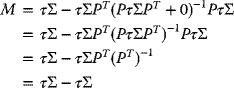
namely,
And if the investor is not confident in the views, Ω → ∞, then (3.113) can be reduced to
namely,
Alternative Reference Model
Consider now the most common alternative reference model used with the Black–Litterman estimation model: It is the one used in Satchell and Scowcroft (2000), and in the work of Meucci prior to his introduction of “Beyond Black–Litterman”:
In this reference model, µ is normally distributed with variance ∑. One may estimate µ, but µ is not considered a random variable. This is commonly described as having a τ = 1, but more precisely one is making a point estimate and thus have eliminated τ as a parameter. In this model, Ω becomes the covariance of the returns to the views around the unknown mean return,, just as ∑ is the covariance of the prior return about its mean. Given that one is now using point estimates, the posterior is now a point estimate and one no longer needs to be concerned about posterior covariance of the estimate. In this model, one does not have a posterior precision to use downstream in one's portfolio selection model.
Rewriting Equation (3.105):
noting that one may move around the τ term:
Now it is seen that τ only appears in one term in this formula. Because the Alternative Reference Model does not include updating the covariance of the estimates, this is the only formula. Given that the investor is selecting both Ω and τ to control the blending of the prior and their views, one may eliminate one of the terms. Since τ is a single term for all views and Ω has a separate element for each view, one shall keep Ω. One may then rewrite the posterior estimate of the mean as follows:
The primary artifacts of this new reference model are as follows:
- τ is gone.
- The investor's portfolio weights in the absence of views equal the equilibrium portfolio weights.
- Finally, at implementation time, there is no need or use of (3.106) or (3.107).
Remark:
- None of the authors prior to Meucci (2008), except for Black and Litterman (1992) and He and Litterman (1999), make any mention of the details of the Canonical Reference Model or of the fact that different authors actually use quite different reference models.
- In the Canonical Reference Model, the updated posterior covariance of the unknown mean about the estimate will be smaller than the covariance of either the prior or conditional estimates, indicating that the addition of more information will reduce the uncertainty of the model. The variance of the returns from (3.107) will never be less than the prior variance of returns. This matches the intuition as adding more information should reduce the uncertainty of the estimates.
- Since there is some uncertainty in this value (M), (3.107) provides a better estimator of the variance of returns than the prior variance of returns.
Impact of τ
For users of the Black–Litterman model, the meaning and impact of the parameter τ may cause confusion. Investors using the Canonical Reference Model use τ and that it does have a very precise meaning in the model. An author who selects an essentially random value for τ probably does not using the Canonical Reference Model, but instead uses the Alternative Reference Model.
Given the Canonical Reference Model, one may still understand the impact of τ on the results. One may start with the expression for Ω similar to the one used by He and Litterman (1999). Rather than using only the diagonal, one may retain the entire structure of the covariance matrix to simplify the methodology:
One may substitute (3.108) into (3.105):
to obtain

namely,
Thus, using (3.108) is just a simplification and does not do justice to investors' views, but one may still see that setting Ω proportional to τ will eliminate τ from the final formula for ∏.
In the Canonical Reference Model, it does not eliminate τ from the equations for posterior covariance given by (3.107):
In the general form, if one formulates Ω as
then one may rewrite (3.109) as
One may see a similar result if one substitutes Equation (3.108) into Equation (3.113):
Resulting in:

namely,
Note that τ is not eliminated from (3.117). One may also observe that if τ is on the order of 1, and if one were to use the equation
then the uncertainty in the estimate of the mean would be a significant portion of the variance of the returns. With the Alternate Reference Model, no posterior variance computations are preformed and the mixing is weighted by the variance of returns.
In both cases, the choice for Ω has evenly weighted the prior and conditional distributions in the estimation of the posterior distribution. This matches the intuition when one considers one has blended two inputs, for both of which one has the same level of uncertainty. The posterior distribution will be the average of the two distributions. If instead one solves for the more useful general case of
where α ≥ 0, substituting into (3.105) and following the same logic as used to derive (3.117) one obtains
This parameterization of the uncertainty is specified in Meucci (2005) and it allows us an option between using the same uncertainty for the prior and views, and having to specify a separate and unique uncertainty for each view. Given that one is essentially multiplying the prior covariance matrix by a constant, this parameterization of the uncertainty of the views does not have a negative impact on the stability of the results.
Note that this specification of the uncertainty in the views changes the assumption from the views being uncorrelated to the views having the same correlations as the prior returns.
In summary, if the investor uses the Alternative Reference Model and makes Ω proportional to ∑, then it is necessary only to calibrate the constant of proportionality, α, which indicates their relative confidence in their views versus the equilibrium. If the Canonical Reference Model is used and set Ω proportional to τ∑, then the return estimate will not depend on the value of τ, but the posterior covariance of returns will depend on the proper calibration of τ.
Calibration of τ
Some empirical ways to select and calibrate the value of τ will be considered:
The first method to calibrate τ relies on basic statistics: When estimating the mean of a distribution, the uncertainty (variance) of the mean estimate will be proportional to the inverse of the sample sizes. Given that one is estimating the covariance matrix from historical data, then
| τ = 1/T | The maximum-likelihood estimator |
| τ = 1/(T − k) | The best quadratic unbiased estimator |
where T = the number of samples and k = the number of assets.
While there are other estimators, usually the first definition above is used. Given that one usually aims for a number of samples around 60 (viz., 5 years of 12 monthly samples), τ is on the order of 0.02 (1/60 = 0.01666…). This is consistent with several of the papers that indicate they used values of τ on the range of (0.025, 0.05).
The most intuitively easy way to calibrate τ is as part of a confidence interval for the prior mean estimates. One may illustrate this concept with a simple example: Consider the scenario where τ = 0.05, and one considers only a single asset with a prior estimate of 7% as the excess return and 15% as the known standard deviation of returns about the mean. If one uses a confidence interval of (1%, 5%) with 68% confidence, one keeps the ratio of View Precision to Prior Precision fixed between the two scenarios, one with τ = 0.05 and one with τ = 1. In the first scenario, even though one uses a seemingly small τ = 0.05, the prior estimate has relatively low precision based on the width of the confidence interval, and thus the posterior estimate will be heavily weighted toward the view. In the second scenario with τ = 1, the prior confidence interval is so wide as to make the prior estimate close to worthless. In order to keep the posterior estimate the same across scenarios, the view estimate also has a wide confidence interval indicating the investor is really not confident in any of their estimates!
Remarks:
- One could instead calibrate τ to the amount invested in the risk-free asset given the prior distribution. Here one sees that the portfolio invested in risky assets given the prior views will be
(3.120)
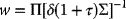
- Thus, the weights allocated to the assets are smaller by [1/(1+τ)] than the CAPM market weights. This is on account of the Bayesian investor is uncertain in the estimate of the prior and does not want to be 100% invested in risky assets.
Results
It is of interest and considerable enlightenment to review and compare the results of the various authors on this subject. The Java programs used to compute these results are all available as part of the akutan open source finance project at ∏ sourceforge.net. All of the mathematical functions were built using the Colt open-source numerics library for Java. Selected formulas are also available as MATLAB and/or SciLab scripts on the website blacklitterman.org. Any small differences between all the authors' reported results are most likely the result of rounding of inputs and/or results. When reporting results, most authors have just reported the portfolio weights from an unconstrained optimization using the posterior mean and variance. Given that the vector ∏ is the excess return vector, one does not need a budget constraint (∑wi = 1) as one may safely assume any “missing” weight is invested in the risk-free asset that has expected return 0 and variance 0. This calculation comes from (3.86b):
or
As a first test of the algorithm, one verifies that when the investor has no views that the weights are correct, substituting (3.109) into (3.86b)
one obtains
or
Hence, it is clear that the output weights with no views will be impacted by the choice of τ when the Black–Litterman reference model is used. He and Litterman (1999) indicate that if the investor is a Bayesian, then one shall not be certain of the prior distribution and thus would not be fully invested in the risky portfolio in the beginning. This is consistent with (3.121).
Matching the Results of He and Litterman
First one shall consider the results shown in He and Litterman (1999). These results are easy to reproduce as they clearly implement the Canonical Reference Model and they provide all the data required to reproduce their results in the paper.
He and Litterman (1999) set
This makes the uncertainty of the views equivalent to the uncertainty of the Equilibrium estimates. A small value for τ, 0.05, was selected, and the Canonical Reference Model was used. The updated posterior variance of returns is calculated in (3.113) and (3.107).
The results of Table 3.5 correspond to Table 7 in (He and Litterman, 1999).
Table 3.5 Results computed using the akutan implementation of Black–Litterman and the input data for the equilibrium case and the investor's views from He and Litterman (1999).
| Asset | P0 | P1 | µ | weq/(1+τ) | w* | w*- weq/(1+τ) |
| Australia | 0.0 | 0.0 | 4.3 | 16.4% | 1.5% | 0.0% |
| Canada | 0.0 | 1.0 | 8.9 | 2.1% | 53.9% | 51.8% |
| France | −0.295 | 0.0 | 9.3 | 5.0% | −0.5% | −5.4% |
| Germany | 1.0 | 0.0 | 10.6 | 5.2% | 23.6% | 18.4% |
| Japan | 0.0 | 0.0 | 4.6 | 11.0% | 11.0% | 0.0% |
| UK | −0.705 | 0.0 | 6.9 | 11.8% | −1.1% | −13.0% |
| USA | 0.0 | −1.0 | 7.1 | 58.6% | 6.8% | −51.8% |
| Q | 5.0 | 4.0 | ||||
| ω/τ | 0.043 | 0.017 | ||||
| λ | 0.193 | 0.544 | ||||
| The values shown for w* exactly match the values shown in their paper: Figure 5—Distributions of actual means about estimates means. | ||||||
Figures 3.30 and 3.31 show the pdf for the prior, view, and posterior for each view defined in the problem. The y-axis uses the same scale in each graph. Note how in Figure 3.27 the conditional distribution of the estimated mean is much more diffuse because the variance of the estimate is larger (viz., precision of the estimate is smaller). Note how the precision of the prior and views impacts the precision (width of the peak) on the pdf. In Figure 3.27 with the less precise view, the posterior is also less precise.
Figure 3.30 Canadian outperforming U.S. equities by 4%.
Figure 3.31 German outperforming other European equities by 5%.
Matching the Results of Idzorek
This section reproduces the results of Idzorek (2005). In trying to match Idzorek's results, it is found that Idzorek used the Alternative Reference Model. which leaves ∑, the known variance of the returns from the prior distribution, as the variance of the posterior returns. This is a significant difference from the Canonical Reference Model, but in the end the differences amounted to only 50 basis points per asset. Tables 3.6 and 3.7 illustrate calculated results with the data from Idzorek's paper and how the results differ between the two versions of the model.
Table 3.6 Canonical Reference model with Idzorek data (corresponds with data in Idzorek's Table 6).
| Asset class | µ | weq | w | Black–Litterman reference model | Idzorek's results |
| U.S. Bonds | 0.07 | 18.87% | 28.96% | 10.09% | 10.54% |
| Intl Bonds | 0.50 | 25.49% | 15.41% | −10.09% | −10.54% |
| US LG | 6.50 | 11.80% | 9.27% | −2.52% | −2.73% |
| US LV | 4.33 | 11.80% | 14.32% | 2.52% | −2.73% |
| US SG | 7.55 | 1.31% | 1.03% | −0.28% | −0.30% |
| US SV | 3.94 | 1.31% | 1.59% | 0.28% | 0.30% |
| Intl Dev | 4.94 | 24.18% | 27.74% | 4.15% | 3.63% |
| Intl Eng | 6.84 | 3.40% | 3.40% | 0% | 0% |
Table 3.7 Alternative Reference model with Idzorek data (corresponds with data in Idzorek's Table 6).
| Country | µ | weq | w | Alternative reference model | Idzorek's results |
| US Bonds | 0.07 | 19.34% | 29.89% | 10.55% | 10.54% |
| Intl Bonds | 0.50 | 26.13% | 15.58% | −10.55% | −10.54% |
| US LG | 6.50 | 12.09% | 9.37% | −2.72% | −2.73% |
| US LV | 4.33 | 12.09% | 14.81% | 2.72% | −2.73% |
| US SG | 7.55 | 1.34% | 1.04% | −0.30% | −0.30% |
| US SV | 3.94 | 1.34% | 1.64% | 0.30% | 0.30% |
| Intl Dev | 4.94 | 24.18% | 27.77% | 3.59% | 3.63% |
| Intl Eng | 6.84 | 3.49% | 3.49% | 0.00% | 0.00% |
Table 3.6 contains results generated using the data from Idzorek (2005) and the Canonical Reference Model. Table 3.7 shows the same results as generated by the Alternative Reference Model.
Note that the results in Table 3.6 are close, but for several of the assets the difference is about 50 basis points. The values shown in Table 3.7 are within four basis points, essentially matching the results reported by Idzorek.
Additional Work
Consider efforts to reproduce results from some of the major research papers on the Black–Litterman model.
Of the major papers on the Black–Litterman model, there are two that would be very useful to reproduce:
- Satchell and Scowcroft (2000)
- Black and Litterman (1992)
Satchell and Scowcroft (2000) did not provide enough data in their paper to reproduce their results. They have several examples, one with 11 countries equity returns plus currency returns, and one with 15 countries. They did not provide the covariance matrix for either example, and so their analysis cannot be reproduced. It would be interesting to confirm that they use the Alternative Reference Model by reproducing their results.
Black and Litterman (1992) did provide what seems to be all the inputs to their analysis, although they chose a nontrivial example, including partially hedged equity and bond returns. This requires the application of some constraints to the reverse optimization process that have been formulated. It should be useful to continue this work with the goal of verifying the details of the Black–Litterman implementation used in Black and Litterman (1992).
Extensions to the Black–Litterman Model
This section covers the extensions to the Black–Litterman model proposed in Idzorek (2005), Fusai and Meucci (2003), Krishnan and Mains (2006), and Qian and Gorman (2001).
Idzorek (2005) presents a means to calibrate the confidence or variance of the investors views in a simple and straightforward method.
Next is a section on measures of extremity or quality of views. Fusai and Meucci (2003) proposed a way to measure how consistent a posterior estimate of the mean is with regard to the prior, or some other estimate. Braga and Natale (2007) described how to use Tracking Error to measure the distance from the equilibrium to the posterior portfolio. Also included are additional original work on using relative entropy to measure quality of the views.
Finally, larger extensions to the model such as Krishnan and Mains (2006) present a method to incorporate additional factors into the model. Qian and Gorman (2001) presented a method to integrate views on the covariance matrix as well as views on the returns.
Idzorek's Extension
Idzorek's apparent goal was to reduce the complexity of the Black–Litterman model for nonquantitative investors. He achieved this by allowing the investor to specify the investors' confidence in the views as a percentage (0–100%) where the confidence measures the change in weight of the posterior from the prior estimate (0%) to the conditional estimate (100%). This linear relation is shown in Equation (3.123):
where
- w100 is the weight of the asset under 100% certainty in the view,
- wmkt is the weight of the asset under no views, and
- w is the weight of the asset under the specified view.
Also provided was a method to back out the value of ω required to generate the proper tilt (change in weights from prior to posterior) for each view. These values may then be combined to form Ω, and the model is used to compute posterior estimates.
Idzorek includes τ in the formulas, but because of the use of the Alternative Reference Model and his formula (3.123), there is no need to use τ with the Idzorek method.
The paper discussed solving for ω using a least-squares method. One may actually solve this analytically. The next section will provide a derivation of the formulas required for this solution.
First one may use the following form of the uncertainty of the views. Idzorek includes τ in this formula, but he uses the Alternative Reference Model so that one may drop τ from the formulation of his method:
where α, the coefficient of uncertainty, is a scalar quantity in the interval [0, ∞].
- When the investor is 100% confident in their views, then α will be 0.
- When they are totally uncertain, then α will be ∞.
Note that (3.124) is exact, it is identical to Equation (3.122) and the Ω used by He and Litterman (1999) because it is a 1 × 1 matrix. This allows one to find a closed-form solution to the problem of Ω for Idzorek's confidence.
First one substitutes (3.119)
into
or
yielding
Now one may solve (3.125) at the boundary conditions for α:
And recombining some of the terms in (3.125), one arrives at
Substituting wmkt and w100, from (3.126) and (3.127) respectively, into (3.128), the result is
And comparing the above with (3.123):
It is seen that
However, if one solves for α from (3.130), one obtains
Using (3.131) and (3.124), the investor can easily calculate the value of ω for each view, and then roll them up into a single Ω matrix. To check the results for each view, one then solve for the posterior estimated returns using (3.105) and plug them back into (3.123). When the investors apply all their views at once, the interaction among the views may pull the posterior estimate for individual assets away from the results generated when the views were taken one at a time.
Idzorek's method greatly simplified the investor's process of specifying the uncertainty in the views when the investor does not have a quantitative model driving the process. In addition, this model does not add meaningful complexity to the process.
An Example of Idzorek's Extension
Idzorek described the steps required to implement his extension in his paper, but did not provide a complete worked example. Here, one will work through the example from where Idozorek left off!
Idzorek's example includes three views:
- International Development Equity will have absolute excess return of 5.25%, Confidence 25.0%.
- International Bonds will outperform U.S. bonds by 25 bps, Confidence 50.0%.
- U.S. Growth Equity will outperform U.S. Value Equity by 2%, Confidence 65.0%.
Idzorek defined the steps that include calculations of w100 and then the calculation of ω for each view given the desired change in the weights. From the previous section, one noted that one only need to take the investor's confidence for each view, plug it into (3.131), and calculate the value of alpha. Then one plugs α, P, and ∑ into Equation (3.124) and compute the value of ω for each view. At this point, one may assemble the Ω matrix and proceed to solve for the posterior returns using (3.104) or (3.105).
In presenting this example, the results for each view will be shown including wmkt and w100 in order to make the working of the extension more transparent. Tables 3.8–3.10 show the results for a single view.
Table 3.8 Calibrated results for View 1.
| Asset | ω | wmkt | w* | w 100% | Implied confidence |
| Intl Dev Equity | 0.002126625 | 24.18% | 25.46% | 29.28% | 25.00% |
Table 3.9 Calibrated results for View 2.
| Asset | ω | wmkt | w* | w 100% | Implied confidence |
| US Bonds | 0.000140650 | 19.34% | 29.06% | 38.78% | 50.00% |
| Intl Bonds | 0.000140650 | 26.13% | 16.41% | 6.69% | 50.00% |
Table 3.10 Calibrated results for View 3.
| Asset | ω | wmkt | w* | w 100% | Implied confidence |
| US LG | 0.000466108 | 12.09% | 9.49% | 8.09% | 65.00% |
| US LV | 0.000466108 | 12.09% | 14.69% | 16.09% | 65.00% |
| US SG | 0.000466108 | 1.34% | 1.05% | 0.90% | 65.00% |
| US SV | 0.000466108 | 1.34% | 1.63% | 1.78% | 65.00% |
Then one may use the freshly computed values for the Ω matrix with all views specified together and arrive at the final result shown in Table 3.11 blending all three views together.
Table 3.11 Final results for Idzorek's confidence extension example.
| Asset | View 1 | View 2 | View 3 | µ | σ | wmkt | Posterior weight | Change |
| US Bonds | 0.0 | −1.0 | 0.0 | 0.1 | 3.2 | 19.3% | 29.6% | 10.3% |
| Intl Bonds | 0.0 | 1.0 | 0.0 | 0.5 | 8.5 | 26.1% | 15.8% | 10.3% |
| US LG | 0.0 | 0.0 | 0.9 | 6.3 | 24.5 | 12.1% | 8.9% | 3.2% |
| US LV | 0.0 | 0.0 | −0.9 | 4.2 | 17.2 | 12.1% | 15.2% | 3.2% |
| US SG | 0.0 | 0.0 | 0.1 | 7.3 | 32.0 | 1.3% | 1.0% | −0.4% |
| US SV | 0.0 | 0.0 | −0.1 | 3.8 | 17.9 | 1.3% | 1.7% | 0.4% |
| Intl Dev | 1.0 | 0.0 | 0.0 | 4.8 | 16.8 | 24.2% | 26.0% | 1.8% |
| Intl Eng | 0.0 | 0.0 | 0.0 | 6.6 | 28.3 | 3.5% | 3.5% | −0% |
| Total | 101.8% | |||||||
| Return | 5.2 | 2 | 2.0 | |||||
| Omega/Tau | 0.08507 | 0.00563 | 0.01864 | |||||
| Lambda | 0.002 | −0.006 | −0.002 |
Impact of the Several Views
Consider the methods used in the literature to measure the impact of the views on the posterior distribution. In general, one may divide these measures into two groups:
- The first group allows one to test the hypothesis that the views or posterior contradict the prior.
- The second group allows one to measure a distance or information content between the prior and posterior.
Theil (1971) and Fusai and Meucci (2003) described measures that are designed to allow a hypothesis test to ensure the views or the posterior does not contradict the prior estimates. Theil (1971) described a method of performing a hypothesis test to verify that the views are compatible with the prior. That work is being extended to measure compatibility of the posterior and the prior. Fusai and Meucci (2003) described a method for testing the compatibility of the posterior and prior when using the alternative reference model. He and Litterman (1999) and Braga and Natale (2007) described measures that may be used to measure the distance between two distributions, or the amount of tilt between the prior and the posterior. These measures did not lend themselves to hypothesis testing, but they may be used as constraints on the optimization process. He and Litterman (1999) define a metric, Λ, which measured the tilt induced in the posterior by each view. Braga and Natale (2007) used Tracking Error Volatility (TEV) to measure the distance from the prior to the posterior.
Theil's Measure of Compatibility Between the Views and the Prior
Theil (1971) described this as testing the compatibility of the views with the prior information. Given the linear mixed estimation model, one has the prior (3.132) and the conditional (3.133):
The mixed estimation model defines u as a random vector with mean 0 and covariance τ∑, and v as a random vector with mean 0 and covariance Ω.
The approach being taken here is very similar to the approach taken when analyzing a prediction from a linear regression. One has two estimates of the views, the conditional estimate of the view and the posterior estimate of the returns.
One may define the posterior estimate as . One may measure the estimation error between the prior and the views as
The vector ζ has mean 0 and variance V(ζ). One shall form one's own hypothesis test using the formulation
The quantity ξ is known as the Mahalanobis distance (multidimensional analog of the z-score) and is distributed as χ2(n). In order to use this form, one needs to solve for the E(ζ) and V(ζ).
If one considers only the information in the views, the estimator of β is
Note that since P is not required to be a matrix of full rank, one might not be able to evaluate this formula as written. One works in return space here (as opposed to view space) as it seems more natural. Later on one will transform the formula into view space to make it computable.
One then substitutes the new estimator into the formula (3.134) and eliminate x as it is the identity matrix in the Black–Litterman application of mixed estimation:
Next one substitutes formula (3.133) for Q.
Given the estimator, one needs to find the variance of the estimator, as follows:
Now, E(vu) = 0, so one may eliminate the cross-term, and simplify the formula:
The last step is to take the expectation of (3.137). At the same time, one will substitute the posterior estimate (µ) for β.
Now substitute the various values into (3.135) as follows:
Unfortunately, under the usual circumstances, one cannot compute ξ. Because P does not need to contain a view on every asset, several of the terms are not always computable as written. However, one may easily convert it to view space by multiplying by P and PT.
This new test statistic ξ in (3.148) is distributed as χ2(q), where q is the number of views. It is the square of the Mahalanobis distance of the posterior return estimate versus the posterior covariance of the estimate. One may use this test statistic to determine if the views are consistent with the prior by means of a standard confidence test:
where F(ξ) is the CDF of the χ2(q) distribution.
One may also calculate the sensitivities of this measure to the views using the chain rule:
Substituting the various terms,
where f(ξ) is the PDF of the χ2(q) distribution.
The Theil Measure of the Source of Posterior Information
Theil (1963) describes a measure that may be used to determine the contribution to the posterior precision of the prior and the views. This measure was called θ sums to 1 across all sources, and conveniently also sums across the views if one measures the contribution of each view.
The measure for the contribution to posterior precision from the prior is
where n is the number of assets. Equation (3.153) can be used for all views by using the full matrices P and Ω. For a single view i, use the relevant slices of P and Ω:
(Equations 3.152) and (3.153) provide the equations one may use to compute the contribution toward the posterior precision from both the prior and the views. One may use this diagnostic to identify if the relative contributions match the intuitive view on this proportion.
Fusai and Meucci's Measure of Consistency
Next consider the work of Fusai and Meucci (2003). In their paper they present a way to quantify the statistical difference between the posterior return estimates and the prior estimates. This provided a way to calibrate the uncertainty of the views and ensured that the posterior estimates are not extreme when viewed in the context of the prior equilibrium estimates.
In this paper they used the Alternative Reference Model. The measure is analogous to Theil's Measure of Compatibility, but because the alternative reference model used the prior variance of returns for the posterior, they did not need any derivation of the variance. One may apply a variant of their measure to the Canonical Reference Model as well. They proposed the use of the squared Mahalanobis distance of the posterior returns from the prior returns. This includes τ to match the Canonical Reference Model, but their work did not include τ as they used the Alternative Reference Model:
It is essentially measuring the distance from the prior, µ, to the estimated returns, µBL, normalized by the uncertainty in the estimate. One may use the covariance matrix of the prior distribution as the uncertainty. The squared Mahalanobis distance is distributed as χ2(q) where q is the number of assets. This may easily be used in a hypothesis test. Thus, the probability of this event occurring can be computed as
where F(M(q)) is the CDF of the chi-square distribution of M(q) with n degrees of freedom.
Finally, to identify which views contribute most highly to the distance away from the equilibrium, one may also compute sensitivities of the probability to each view. Use the chain rule to calculate the partial derivatives
where f(M) is the PDF of the chi-square distribution with n degrees of freedom for M(q). Note that this measure is very similar to (3.151) Theil's measure of compatibility between the prior and the views.
An example in their paper resulted in an initial probability of 94% that the posterior is consistent with the prior. They specified that their investor desires this probability to be no less than 95% (a commonly used confidence level in hypothesis testing), and thus they would adjust their views to bring the probability in line. Given that they also computed sensitivities, their investor can identify that views are providing the largest marginal increase in their measure and the investor may then adjust these views. These sensitivities are especially useful since some views may actually be pulling the posterior toward the prior, and the investor could strengthen these views or weaken views that pull the posterior away from the prior. The last point may seem nonintuitive. Given that the views are indirectly coupled by the covariance matrix, one would expect that the views only push the posterior distribution away from the prior. However, because the views can be conflicting, either directly or via the correlations, any individual view may have a net impact pushing the posterior closer to the prior, or pushing it further away.
They proposed to use their measure in an iterative method to ensure that the posterior is consistent with the prior to the specified confidence level. With the Canonical Reference Model, one could rewrite (3.154) using the posterior variance of the return instead of τ∑ yielding
Otherwise, their Consistency Measure and its use is the same for both reference models.
He and Litterman Lambda
He and Litterman (1999) used a measure, Λ, to measure the impact of each view on the posterior. They defined the Black–Litterman unconstrained posterior portfolio as a blend of the equilibrium portfolio (prior) and a contribution from each view; that contribution is measured by Λ.
Deriving the formula for Λ, one will start with (3.86b) and substitute in the various values from the posterior distribution
and also substitute the return for ∏:
The covariance term will first be simplified:
Then, one may define
And finally rewrite as
One uses the multiplier, {τ/(1+τ)}, because in the Black–Litterman Reference Model the investor is not fully invested in the prior (equilibrium) portfolio.
To find Λ, one may substitute (3.162) into (3.159), and then gather terms:
Thus, along with (3.161), the following equation defines Λ:
Λ, of He and Litterman, represents the weight on each of the view portfolios on the final posterior weight. As a result, one may use Λ as a measure of the impact of one's views.
One may also derive the He and Litterman Λ for the Alternative Reference Model: Call this ΛA. One may start from the same reverse optimization equation3.86b:
and substitute the return from (3.104) for ∏,
but using the prior covariance matrix as 1 is using the Alternative Reference Model.
First simplify the covariance term using the Woodbury Matrix Identity.
Then, one may define
and one may substitute the above result back into (3.128) and expand the terms:
In He and Litterman, Λ took the similar form in the Alternative Reference Model as shown here:
Note that in the Alternative Reference Model, the investor's prior portfolio has the exact same weights as the equilibrium portfolio.
One may note that the following formula defines ΛA:
Braga and Natale and Tracking Error Volatility (TEV)
Braga and Natale (2007) proposed the use of tracking error between the posterior and prior portfolios as a measure of distance from the prior. Tracking error is commonly used by investors to measure risk versus a benchmark, and may be used as an investment constraint. Since it is commonly used, most investors have an intuitive understanding and a level of comfort with TEV.
Tracking Error Volatility (TEV) is here defined as
and where
- wactv is the active weights or active portfolio,
- is the weight in the investor's portfolio,
- wr is the weight in the reference portfolio, and
- ∑ is the covariance matrix of returns.
Moreover, the formula derived for tracking error sensitivities is as follows:Given that
and one may further refine
where q represents the views.
Then one may use the chain rule to decompose the sensitivity of TEV to the views:
Solving for the first term of (3.176) directly,
Let ![]() , then applying the chain rule to solve for the first term of (3.176):
, then applying the chain rule to solve for the first term of (3.176):

And similarly solve for the second term of (3.176):
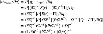
This result differs somewhat from that found in the Braga and Natale (2007) paper because the form of the Black–Litterman model is used that requires less matrix inversions. The sensitivities equation is
One may come up with the equivalent metric for the Canonical Reference Model. Notice that in a tracking error scenario, the covariance matrix should be the most accurate, which would be the posterior covariance matrix:
yielding the TEV sensitivities for the Canonical Reference Model:
Braga and Natale provided an example in their paper, but they did not provide all the raw data required to reproduce their results. Given their posterior distribution as presented in the paper, one should easily reproduce their TEV results. One advantage of the TEV is that most investors are familiar with it, and so they will have some intuition as to what it represents. The consistency metric introduced by Fusai and Meucci (2003) will not be as familiar to investors.
Metrics Introduced in Herold (2003)
This diagnostic concept may be applied to portfolio models in order to validate the outputs. One of these diagnostics is the correlation between views as one diagnostic that may be used to determine how the updated portfolio may perform. By examining the correlation matrix of the views, P ∑ Pt, one may determine how correlated the views are. If the views are highly correlated, then one may expect all views to contribute to the performance if they are correct, and underperformance if they are incorrect. If the views are not highly correlated, then one may expect a diversified contribution to performance.
As an example, if one uses the He and Litterman's data and their two views, one calculated this measure as
The off-diagonal elements (0.0020 and 0.0020) are one order of magnitude smaller than the on-diagonal elements (0.0213 and 0.0170). This difference indicates that the views are not strongly correlated. This is consistent with He and Litterman's specification of the two views on mutually exclusive sets of assets that are loosely correlated.
Herold (2003) also discussed the marginal contribution to tracking error by view. This is the same metric computed by Braga and Natale, although he proposed deriving the formula for its calculation from the Alternative Reference Model version of He and Litterman's Λ, ΛA.
Herold (2003) considers the case of Active Management, which meant that the Black–Litterman model was applied to an active management overlay on some portfolio. The prior distribution in this case corresponds to weq = 0. The posterior weights were the overlay weights. He uses the Alternative Reference Model and computed a quantity Φ, which is the active management version of ΛA.
but weq = 0, so
where
Herold starts from Equation (3.173) just as Braga and Natale, but then uses an alternative formula for tracking error:
and also
Then one may take δTEV/δQ to find the marginal contribution to tracking error by views. By the chain rule:

Note that one could perform the same calculation for the Canonical Reference Model using He and Litterman's Λ, but one would also need to use the posterior covariance of the distribution rather than just ∑ in the calculations.
A Demonstration of the Measures
Consider a sample problem to illustrate all of the metrics, and to provide some comparison of their features. One may start with the equilibrium from He and Litterman (1999) and for Example 1 use the views from their paper; Germany will outperform other European markets by 5% and Canada will outperform the United States by 4%.
Table 3.12 illustrates the results of applying the views and Table 3.13 displays the various impact measures.
Table 3.12 Example 1 returns and weights: equilibrium from He and Litterman (1999).
| Asset | P0 | P1 | µ | µeq | weq/(1+τ) | w* | w* – weq/(1 + τ) |
| Australia | 0.0 | 0.0 | 4.45 | 3.9 | 1.50% | 1.5% | 0.0% |
| Canada | 0.0 | 1.0 | 9.06 | 6.9 | 2.1% | 53.3% | 51.2% |
| France | −0.295 | 0.0 | 9.53 | 8.4 | 5.0% | −3.3% | −8.3% |
| Germany | 1.0 | 0.0 | 11.3 | 9 | 5.2% | 33.1% | 27.9% |
| Japan | 0.0 | 0.0 | 4.65 | 4.3 | 11.0% | 11.0% | 0.0% |
| UK | −0.705 | 0.0 | 6.98 | 6.8 | 11.8% | −7.8% | −19.6% |
| USA | 0.0 | −1.0 | 7.31 | 7.6 | 58.6% | 7.3% | −51.3% |
| q | 5.0 | 4.0 | |||||
| ω/τ | 0.02 | 0.017 |
Table 3.13 Impact measures for Example 1.
| Measure | Value (confidence level) | Sensitivity (V1) | Sensitivity (V2) |
| Theil's measure | 1.672 (43.3%) | −5.988 | −11.46 |
| Theil's θ | 0.858 (prior) | 0.0712 | 0.0712 |
| Fusai and Meucci's measure | 0.8728 (99.7%) | −0.1838 | −0.3327 |
| Λ | 0.2920 | 0.5380 | |
| TEV | 8.28% | 0.688 | 1.294 |
If one examines the change in the estimated returns versus the equilibrium, one sees where the U.S. returns decreased by only 29 bps, but the allocation decreased 51.25% caused by the optimizer favoring Canada whose returns increased by 216 bps and whose allocation increased by 51.25%. This shows that what appear to be moderate changes in return forecasts may cause very large swings in the weights of the assets, a common issue with unconstrained mean variance optimization. Here one uses unconstrained mean variance optimization not because one has to, but because it is well understood and transparent.
Looking at the impact measures, Theil's measure indicates that one may be confident only at the 43% level that the views are consistent with the prior. If one examines the diagram, one may see that indeed these views are significantly different from the prior. Fusai and Meucci's measure of compatibility of the prior and posterior, on the other hand, comes with a confidence level of 99.8%, so they are much more confident that the posterior is consistent with the prior. A major difference in their approaches is that Theil is working in view space, which for the example has order of 2, while Fusai and Meucci are working in asset space which has order of 7.
All of the metrics' sensitivities to the views indicate that the second view has a relative weight just about twice as large as the first view, so the second view contributes much more to the change in the weights.
The TEV of the posterior portfolio is 8.28%, which is significant in terms of how closely the posterior portfolio will track the equilibrium portfolio. This seems to be a very large TEV value given the scenario with which one is working. Next, one changes one's confidence in the views by multiplying the variance by 2, this will increase the change from the prior to the posterior and allow one to make some judgments based on the impact measures.
Examining the updated results in Table 3.14, one sees that the changes to the forecast returns have decreased—consistent with the increased uncertainty in the views. One now has a 20% increase in the allocation to Canada and a 20% decrease in the allocation to the United States. From Table 3.15, one may see that Theil's measure has increased, but only by a fraction and one continues to have little confidence that the views are consistent with the prior. Fusai and Meucci's measure now is 99.8% confident that the posterior is consistent with the prior. It is unclear in practice what bound one would want to use, but their measure usually presents with a much higher confidence than Theil's measure. The TEV has decreased and is now 7.67%, which is not significantly smaller.
Table 3.14 Example 2 returns and weights: equilibrium from He and Litterman, (1999).
| Asset | P0 | P1 | µ | weq/(1 + τ) | w* | w* – weq/(1 + τ) |
| Australia | 0.0 | 0.0 | 4.72 | 1.5% | 1.5% | 0.0% |
| Canada | 0.0 | 1.0 | 10.3 | 2.1% | 22.7% | 20.6% |
| France | −0.295 | 0.0 | 10.2 | 5.0% | 1.6% | −3.4% |
| Germany | 1.0 | 0.0 | 12.4 | 5.2% | 16.8% | 11.6% |
| Japan | 0.0 | 0.0 | 4.84 | 11.0% | 11.0% | 0.0% |
| UK | −0.705 | 0.0 | 7.09 | 11.8% | 3.7% | −8.1% |
| USA | 0.0 | −1.0 | 7.14 | 58.6% | 38.0% | −20.6% |
| q | 5.0 | 4.0 | ||||
| ω/τ | 0.09 | 0.07 |
Table 3.15 Impact measures for Example 2.
| Measure | Value (confidence level) | Sensitivity | Sensitivity |
| Theil's measure | 1.537 (46.4%) | −4.27 | −12.39 |
| Theils θ | 0.88 | 0.05 | 0.07 |
| Fusai and Meucci's measure | 0.7479 (99.8%) | −0.06 | −0.24 |
| Λ | 0.193 | 0.544 | |
| TEV | 7.67% | 0.332 | 1.406 |
Once again all the sensitivities show the second view having more of an impact on the final weights.
Across both scenarios, one may draw some conclusions about these various measures. Theil's consistency measure test ranged from a high of 46% confident to a low of 44% confident that the views were consistent with the prior estimates.
This measure is very sensitive and it is unclear what would be a good confidence threshold. “50%” does seem intuitively appealing.
Fusai and Meucci's Consistency measure ranged from 98.38 to 99.98% confident, indicating that the posterior estimates was generally highly consistent with the prior. Fusai and Meucci present that an investor may have a requirement that the confidence level be 5%. In light of these results, that would seem to be a fairly large value. The sensitivities of the Consistency measure scale with the measure, and for low values of the measure the sensitivities are very low.
Theil's θ changed with the confidence of the views and generally indicated that much of the information in the posterior originated with the prior. It moved intuitively with the changes in confidence level.
Across the two scenarios, the TEV decreased by 61 bps, but against a starting point of 8.28%, it still indicates large active weights. It is not clear what a realistic threshold for the TEV is in this case, but these values are likely toward the upper limit that would be tolerated. Note that between the two scenarios, the sensitivity to the first view dropped by 50%, which is consistent with the change in confidence that we applied.
In analyzing these various measures of the tilt caused by the views, the TEV of the weights measures the impact of the views and the optimization process, which one may consider as the final outputs. If the investor is concerned about limits on TEV, they could be easily added as constraints on the optimization process.
He and Litterman's Lambda measures the weight of the view on the posterior weights, but only in the case of an unconstrained optimization. This makes it suitable for measuring impact and being a part of the process, but it cannot be used as a constraint in the optimization process. Theil's compatibility measure and Fusai and Meucci's consistency measure the posterior distribution, including the returns and the covariance matrix: the former in view space, the latter in asset space.
Active Management and the Black–Litterman Model
Active Management refers to the case when the investor is managing an overlay portfolio on top of a 100% invested passive benchmark portfolio. In this case, one is only interested in the overlay and not in the benchmark, so one starts with a prior distribution with 0 active weights and 0 expected excess returns over the benchmark. All returns to views input to the model are relative to the equilibrium benchmark returns rather than to the risk-free rate. The weights are for the active portfolio, so the weights should always sum to 0.
Herold (2003) discusses the application of the Black–Litterman model to the problem of Active Management. He introduces a measure Φ, which is He and Litterman's ΛA modified for Active Management. When one uses the Black–Litterman model for Active Management versus a passive benchmark portfolio, then the equilibrium weights (weq) are 0, and thus the equilibrium returns (∏) are also 0.
Because the value ∏ = 0, the middle term in He and Litterman's ΛA vanishes, and
Two-Factor Black–Litterman
Krishnan and Mains (2005) developed an extension to the alternative reference model that allows the inclusion of additional uncorrelated market factors. The main point involved was that the Black–Litterman model measures risk, like all MVO approaches, as the covariance of the assets. They advocated for a richer measure of risk. They specifically focus on a recession indicator, given the thesis that many investors want assets that perform well during recessions and thus there is a positive risk premium associated with holding assets that do poorly during recessions. Their approach is general and may be applied to one or more additional market factors given that the market has zero beta to the factor and the factor has a nonzero risk premium.
They started from the standard quadratic utility function, but add an additional term for the new market factors:
where
- U is the investors utility, the objective function during portfolio optimization,
- w is the vector of weights invested in each asset,
- ∏ is the vector of equilibrium excess returns for each asset,
- ∑ is the covariance matrix for the assets,
- δ0 is the risk aversion parameter of the market,
- δj is the risk aversion parameter for the jth additional risk factor, and
- βj is the vector of exposures to the jth additional risk factor.
Given their utility function as shown in (3.191), one may take the first derivative with respect to w in order to solve for the equilibrium asset returns.
Comparing this with (3.83)
the simple reverse optimization formula, one sees that the equilibrium excess return vector (∏) is a linear composition of (3.83) and a term linear in the βj values. This matches the intuition as expect assets exposed to this extra factor to have additional return above the equilibrium return.
The following quantities will be further defined as follows:
- rm is the return of the market portfolio,
- fj is the time series of returns for the factor, and
- rj is the return of the replicating portfolio for risk factor j.
In order to compute the values of δ, one will need to perform a little more algebra. Given that the market has no exposure to the factor, one may find a weight vector vj such that vjTβj = 0. In order to find vj, one performs a least-squares fit of ![]() subject to the above constraint. v0 will be the market portfolio
subject to the above constraint. v0 will be the market portfolio
and
One may solve for the various values of δ by multiplying (3.192) by v and solving for δ0:
By construction, v0βj = 0 and v0 ∏ = rm, so
For any j ≥ 1, one may multiply (3.192) by vj and substitute δ0 to obtain
As these factors must all be independent and uncorrelated,
so that one may solve for each δj given by
It was indicated that this is only an approximation because the quantity ![]() may not be identical to 0. The assertion that viβj = 0 ∀ i ≠ j may also not be satisfied for all i and j. For the case of a single additional factor, one can ignore the latter issue.
may not be identical to 0. The assertion that viβj = 0 ∀ i ≠ j may also not be satisfied for all i and j. For the case of a single additional factor, one can ignore the latter issue.
In order to transform these formulas so that one may directly use the Black–Litterman model, Krishnan and Mains changed variables, letting
Substituting back into (3.191), one is back to the standard utility function:
and from (3.85):
one has
and therefore
Given the additional factors, one may then directly substitute and into (3.106) for the posterior returns in the Black–Litterman model in order to calculate the returns:
Note that the additional factors do not impact the posterior variance in any way.
Krishnan and Mains offered an example of their model for world equity models with an additional recession factor. This factor is comprised of the Altman Distressed Debt index and a short position in the S&P 500 index to ensure the market has a zero beta to the factor. They worked through the problem for the case of 100% certainty in the views. They provided all of the data needed to reproduce their results given the set of formulas in this section. In order to perform all the regressions, one would need to have access to the Altman Distressed Debt index along with the other indices used in their paper.
The Work of Qian and Gorman
Qian and Gorman (2001) discussed a method to provide both a conditional mean estimate and a conditional covariance estimate. They used a Bayesian framework referencing the Black–Litterman model, as well as using the alternative reference model as τ did not appear in their paper and they neglected the conditional (or posterior) covariance estimate.
In this section, one will compare the Qian and Gorman approach with the approach taken in the Black–Litterman Reference Model.
One may match the variance portion of Qian and Gorman's formula (3.204) with Equation (3.113):
if one sets Ω = 0, and remove τ (this is the alternative reference model). This describes the scenario where the investor has 100% confidence in their views. For those assets where the investor has absolute views, the variance of the posterior estimate will be zero. For all other assets, the posterior variance will be nonzero.
where
setting Ω = 0 and removing τ:
In order to get Qian and Gorman's Equation (3.207), one needs to reintroduce the covariance of the views, Ω, but rather than mixing the covariances as is done in the Black–Litterman model, one may rely on the lack of correlation and just add the two variance terms. One takes the variance of the conditional from (3.85).
Note that (3.115c) exactly matches (3.207):
where
Upon substituting these into (3.207), the result is
Qian and Gorman demonstrated a conditional covariance that is not derived from Theil's mixed estimation nor from Bayesian updating. Its behavior may increase the variance of the posterior versus the prior in the event that the view variance is larger than the prior variance. They described this as allowing the investor to have a view on the variance, and they do not suggest that Ω needs to be diagonal. In this model the conditional covariance is proportional to the investor's views on variance, but the blending process is not clear.
Compare this formula with (3.113) for the variance of the posterior mean estimate:
Intuition indicates that the updated posterior estimate of the mean will be more precise (viz., lower variance) than the prior estimate, thus one would like the posterior (conditional) variance to always be less than the prior variance. The Black–Litterman posterior variance achieves this goal and arrives at the well-known result of Bayesian analysis in the case of unknown mean and known precision. As a result, it seems one should prefer these results over Qian and Gorman.
Directions for the Future
Future directions for this research include reproducing the results from the original papers: Black and Litterman (1991) and Black and Litterman (1992). These results have the additional complication of including currency returns and partial hedging.
Future work should include more information on process and a synthesized model containing the best elements from the various authors. A full example from the CAPM equilibrium, through the views to the final optimized weights would be useful, and a worked example of the two-factor model from Krishnan and Mains (2005) would also be useful. Meucci (2006, 2008) provides further extensions to the Black–Litterman model for nonnormal views and views on parameters other than return. This allowed one to apply the Black–Litterman model to new areas such as alternative investments or derivatives pricing. His methods are based on simulation and do not provide a closed-form solution.
An Asset Allocation Process Using the Black–Litterman Model
When used as part of an asset allocation process, the Black–Litterman model provided for estimates that lead to more stable and more diversified portfolios than estimates derived from historical returns when used with unconstrained mean-variance optimization. Owing to this significant property, an investor using mean-variance optimization is less likely to require artificial constraints to get a portfolio without extreme weights. Unfortunately, this model requires a broad variety of data, some of which may not be readily available!
- First, the investor needs to identify their investable universe and find the market capitalization of each asset. Then, they need to estimate a covariance matrix for the excess returns of the assets. This is most often done using historical data for an appropriate time window: Both Litterman (2003) and Bevan and Winkelmann (1998) provided details on the process used to compute covariance matrices at Goldman Sachs.
- In the literature, monthly covariance matrices are most commonly estimated from 60 months of historical excess returns.
- If the actual asset return itself cannot be used, then an appropriate proxy can be used, for example, S&P 500 Index for U.S. Domestic Large Cap equities. The return on a short-term sovereign bond, for example, U.S. 4- or 13-week treasury bill, would suffice for most U.S. investor's risk-free rate.
- When applied to the asset allocation problem, finding the market capitalization information for liquid asset classes might be a challenge for an individual investor, but likely presents little obstacle for an institutional investor because of their access to index information from the various providers.
- Given the limited availability of market capitalization data for illiquid asset classes, for example, real estate, private equity, commodities, even institutional investors might have a difficult time piecing together adequate market capitalization information.
- Return data for these same asset classes can also be complicated by delays, smoothing, and inconsistencies in reporting.
- Further complicating the problem is the question of how to deal with hedge funds or absolute return managers. The question of whether they should be considered a separate asset class calls for further research!
- Next, the investor needs to quantify their views so that they can be applied and new return estimates computed. The views can be derived from quantitative or qualitative processes, and can be complete or incomplete, or even conflicting.
- Finally, the outputs from the model need to be fed into a portfolio selection model to generate the efficient frontier, and an efficient portfolio selected.
- Bevan and Winkelmann (1999) provided a description of their asset allocation process (for international fixed income) and how they use the Black–Litterman model within that process. This includes their approaches to calibrating the model and information on how they compute the covariance matrices. The standard Black–Litterman model does not provide direct sensitivity of the prior to market factors besides the asset returns. It is fairly simple to extend the Black–Litterman model to use a multifactor model for the prior distribution. Krishnan and Mains (2005) have provided extensions to the model that allow adding additional cross-asset factors that are not priced in the market.
- Examples of such factors are a recession, or credit, market factor. Their approach is general and could be applied to other factors if desired. Most of the Black–Litterman literature reports results using the closed-form solution for unconstrained mean variance optimization. They also tend to use nonextreme views in their examples.
- As part of an investment process, it is reasonable to conclude that some constraints would be applied at least in terms of restricting short selling and limiting concentration in asset classes. Lack of a budget constraint is also consistent with a Bayesian investor who may not wish to be 100% invested in the market due to uncertainty about their beliefs in the market.
- Portfolio selection is normally considered as part of a two-step process: first compute the optimal portfolio, and then determine position along the Capital Market Line.
Remarks:
- For the ensuing discussion, we will refer to the CAPM equilibrium distribution as the prior distribution, and the investors views as the conditional distribution.
- This is consistent with the original Black and Litterman (1992) papers. It is also consistent with one's intuition about the outcome in the absence of a conditional distribution (no views in Black–Litterman terminology.) This is the opposite to the way most examples of Bayes' theorem are defined: they start with a nonstatistical prior distribution and then add a sampled (statistical) distribution of new data as the conditional distribution. The mixing model and the use of normal distributions will bring the investigation to the same outcome independent of these choices.
Final Remarks on an Asset Allocation Process
The Black–Litterman model is just one part of an asset allocation process. Bevan and Winkelmann (1998) documented the asset allocation process they used in the Fixed Income Group at Goldman Sachs. At a minimum. a Black–Litterman-oriented investment process would have the following steps:
- Determine which assets constitute the market.
- Compute the historical covariance matrix for the assets.
- Determine the market capitalization for each asset class.
- Use reverse optimization to compute the CAPM equilibrium returns for the assets.
- Specify views on the market.
- Blend the CAPM equilibrium returns with the views using the Black–Litterman Model.
- Feed the estimates (estimated returns, covariances) generated by the Black–Litterman model into a portfolio optimizer.
- Select the efficient portfolio that matches the investors' risk preferences.
A further discussion of each step is provided below:
- The first step is to determine the scope of the market. For an asset allocation exercise, this would be identifying the individual asset classes to be considered.
- For each asset class, the weight of the asset class in the market portfolio is required. Then a suitable proxy return series for the excess returns of the asset class is required.
- Between these two requirements, it can be very difficult to integrate illiquid asset classes such as private equity or real estate into the model. Furthermore, separating public real estate holdings from equity holdings (e.g., REITS in the S&P 500 index) may also be required.
- Idzorek (2006) provides an example of the analysis required to include commodities as an asset class. Once the proxy return series have been identified, and returns in excess of the risk-free rate have been calculated, a covariance matrix can be calculated. Typically, the covariance matrix is calculated from the highest frequency data available, for example, daily, and then scaled up to the appropriate time frame.
- Investor's often use an exponential weighting scheme to provide increased weights to more recent data and less to older data. Other filtering (Random Matrix Theory) or shrinkage methods could also be used in an attempt to impart additional stability to the process.
- Now one may run a reverse optimization on the market portfolio to compute the equilibrium excess returns for each asset class. Part of this step includes computing a δ value for the market portfolio. This may be calculated from the return and standard deviation of the market portfolio. Bevan and Winkelmann (1998) discussed the use of an expected Sharpe Ratio target for the calibration of δ.
- For their international fixed income investments, they used an expect Sharpe Ratio of 1.0 for the market. The investor then needs to calibrate τ in some manner. This value is usually on the order of 0.025–0.050. At this point, almost all of the machinery is in place. The investor needs to specify views on the market.
- These views can impact one or more assets, in any combination. The views can be consistent, or they can conflict. An example of conflicting views would be merging opinions from multiple analysts, where they may not all agree. The investor needs to specify the assets involved in each view, the absolute or relative return of the view, and their uncertainty in the return for the view consistent with their reference model and measured by one of the methods discussed previously.
3.6 The Black–Litterman Model
3.6.1 Derivation of the Black–Litterman Model
3.6.1.1 Derivation Using Theil's Mixed Estimation
This discussion includes the derivation of the Black–Litterman master formula (3.58) using Theil's Mixed Estimation approach that is based on Generalized Least Squares.
Theil's Mixed Estimation Approach
This approach is from Theil (1971) and is similar to the reference in the original Black and Litterman (1992) papers. Koch (2005) also includes a derivation similar to this.
Start with a prior distribution for the returns. Assume a linear model such as
where π is the mean of the prior return distribution, β is the expected return, and u is the normally distributed residual with mean 0 and variance Φ.
Next, let one consider some additional information, the conditional distribution:
where q is the mean of the conditional distribution and v is the normally distributed residual with mean 0 and variance Ω.
Both Ω and ∑ are assumed to be nonsingular.
One may combine the prior and conditional information by writing
where the expected value of the residual is 0, and the expected value of the variance is given by
One may then apply the generalized least-squares procedure, which leads to the estimating of β as
which may be rewritten without the matrix notation as
One may derive the expression for the variance using similar logic. Given that the variance is the expectation of ( − β)2, one may start by substituting (3.122) into (3.123), obtaining
namely,
The variance is the expectation of (3.125) squared.

From the foregoing assumptions that E[uu′] = Φ, E[vv′] = Ω, and E(uv′) = 0—because u and v are independent variables, taking the expectations one sees the cross-terms are 0, so that (3.126) becomes
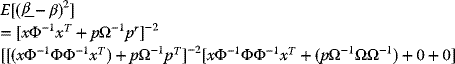
And for the Black–Litterman model, x is the identity matrix and Φ = τ∑ . Upon making these substitutions, the result is
3.6.1.2 Derivation Using Bayes' Theory
This derivation provides an overview of the relevant portion of Bayes' theory in order to create a common vocabulary that may be used in analyzing the Black–Litterman model from a Bayesian viewpoint.
Introduction to Bayes' Theory
Bayes' theory states
in which
- P(A|B) is the conditional (or joint) probability of A, given B, it is also known as the posterior distribution.
- P(B|A) is the conditional probability of B given A, it is also known as the sampling distribution. Call this the conditional distribution.
- P(A) is the probability of A, also known as the prior distribution. Call this the prior distribution.
- P(B) is the probability of B, it is also known as the normalizing constant.
When applying this formula and solving for the posterior distribution, the normalizing constant will disappear into the constants of integration; so from this point on, it may be ignored.
A general problem in using Bayes' theory is to identify an intuitive and tractable prior distribution. One of the core assumptions of the Black–Litterman model (and Mean-Variance optimization) is that asset returns are normally distributed. For that reason, one confines to the case of normally distributed conditional and prior distributions. Given that the inputs are normal distributions, it follows that the posterior will also be normally distributed. When the prior distribution and the posterior have the same structure, the prior is known as a conjugate prior.
Given interest, there is nothing to keep us from building variants of the Black–Litterman model using different distributions; however, the normal distribution is generally the most straightforward.
Another core assumption of the Black–Litterman model is that the variance of the prior and the conditional distributions about the actual mean are known, but the actual mean is not known. This case, known as “Unknown Mean and Known Variance,” is well documented in the Bayesian literature. This matches the model that Theil uses where one has an uncertain estimate of the mean, but know the variance.
Remarks: The significant distributions are defined here below:
- The prior distribution
(3.131)
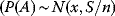
where S is the sample variance of the distribution about the mean, with n samples, then S/n is the variance of the estimate of x about the mean.
The conditional distribution
(3.132)
where Ω is the uncertainty in the estimate µ of the mean, it is not the variance of the distribution about the mean.
- Then the posterior distribution is specified by
(3.133)

- The variance term in (3.133) is the variance of the estimated mean about the actual mean. In Bayesian statistics, the inverse of the variance is known as the precision. One may describe the posterior mean as the weighted mean of the prior and conditional means, where the weighting factor is the respective precision.
- Furthermore, the posterior precision is the sum of the prior and conditional precision. Equation (3.133) requires that the precision of the prior and conditional be noninfinite, and that the sum is nonzero. Infinite precision corresponds to a variance of 0, or absolute confidence.
- Zero precision corresponds to infinite variance, or total uncertainty. As a first check on the formulas, one may test the boundary conditions to see if they agree with one's intuition. If one examines (3.133) in the absence of a conditional distribution, it should collapse into the prior distribution.
(3.134)
 (3.135)
As one may see in Equation (3.133), it does indeed collapse to the prior distribution. Another important scenario is the case of 100% certainty of the conditional distribution, where S, or some portion of it is 0, and thus S is not invertible. One may transform the returns and variance from formula (3.133) into a form more easy to work within the 100% certainty case.
This transformation relies on the result that
It is easy to see that when S is 0 (viz., 100% confidence in the views), the posterior variance will be 0. If Ω is positive infinity (the confidence in the views is 0%), the posterior variance will be (S/n).
Later, one will revisit (Equations 3.133) and (3.136) where one transforms these basic equations into the various parts of the Black–Litterman model. Equation (3.122) contains derivations of the alternative Black–Litterman formulas from the standard form, analogous to the transformation from (3.133) to (3.136).
3.6.2 Further Discussions on The Black–Litterman Model
This section contains a derivation of the Black–Litterman master equation using the standard Bayesian approach for modeling the posterior of two normal distributions. One additional derivation is in Mankert (2006) where the author derived the Black–Litterman “master formula” from Sampling theory, and also shows the detailed transformation between the two forms of this formula.
The PDF-Based Approach
The PDF-based approach follows a Bayesian approach to obtain the PDF of the posterior distribution, when the prior and conditional distributions are both normally distributed. This section is based on the proof shown in DeGroot (1970). This is similar to the approach taken in Satchell and Scowcroft (2000).
This proof examines all the terms in the PDF of each distribution that depends on E(r), neglecting the other terms as they have no dependence on E(r) and thus are constant with respect to E(r).
Starting with the prior distribution, one derives an expression proportional to the value of the PDF:
with n samples from the population.
So ξ(x) from the PDF of P(A) satisfies ∑:
Next, consider the PDF for the conditional distribution:
So ξ(µ|x) from the PDF of P(B|A) satisfies
Substituting (3.139) and (3.141) into (3.75) from the text,
one has an expression which the PDF of the posterior distribution will satisfy.
or
Considering only the quantity in the exponent and simplifying
introduce a new term y, where
and then substitute in the second term:
Then add
giving

The second term has no dependency on E(r), thus it may be included in the proportionality factor and one is left with
Thus, the posterior mean is y and the variance is
3.6.2.1 An Alternative Formulation of the Black–Litterman Formula
This is a derivation of the alternative formulation of the Black–Litterman master formula for the posterior expected return. Starting from (3.104), one will derive formula (3.105):
Separating the parts of the second term:
Replacing the precision term in the first term with the alternative form:
which is the alternative form of the Black–Litterman formula for expected return:
3.6.2.2 A Fundamental Relationship: rA ∼ N{∏, (1 + τ)∑}
This is a derivation of Equation (3.88):
Starting with the definition of the views.
for which
- Q is the k × 1 vector of the unknown mean returns to the views,
- Q is the k × 1 vector of the estimated mean returns to the views,
 is the n × 1 matrix of residuals from the regression where E(
 ) = 0, V(
 ) = E(
 ) = Ω, and
- Ω is nonsingular.
One may rewrite (3.75) into a distribution of Q as follows:
One may also write the definition of the unknown mean returns of the views based on the unknown mean returns of the assets and the portfolio pick matrix P:
where
- P is the k × n vector of weights for the view portfolios, and
- ∏ is the n × 1 vector of the unknown returns of the assets.
Substituting Equation (3.157) into (3.158), one obtains the following:
Assuming that P is invertible, which requires it to be of full rank, then one may multiply both sides by P−1. This is the projection of the view estimated means into asset space representing the Black–Litterman conditional distribution. If P is not invertible, then one would need a slightly different formulation here, adding another term to the right-hand side.
One would like to represent (3.160) as a distribution. In order to do this, one needs to compute the covariance of the random term. The variance of the unknown asset means about the estimated view means projected into asset space is calculated as follows:
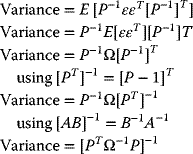
So one arrives at the projection of the views into asset space as (3.162) follows:
The covariance term here is the covariance of the unknown mean returns about the estimated returns from the views, it is not the covariance of expected returns.
3.6.2.3 On Implementing the Black–Litterman Model
Given the following inputs:
| w | Equilibrium weights for each asset class; derived from capitalization-weighted CAPM Market portfolio |
| ∑ | Matrix of covariances between the asset classes; can be computed from historical data |
| rf | Risk-free rate for base currency |
| δ | The risk aversion coefficient of the market portfolio; this may be assumed, or can be computed if one knows the return and standard deviation of the market portfolio |
| τ | A measure of uncertainty of the equilibrium variance; usually set to a small number on the order of 0.025–0.050. |
First, one uses reverse optimization to compute the vector of equilibrium returns, ∏, using Equation (3.163):
Then one formulates the investors views, and specify P, Ω, and Q. Given k views and n assets, then P is a k × n matrix where each row sums to 0 (relative view) or 1 (absolute view). Q is a k × 1 vector of the excess returns for each view. Ω is a diagonal k × k matrix of the variance of the views, or the confidence in the views. To start with, most authors call for the values of ωi to be set equal to pTτ∑ip (where p is the row from P for the specific view).
Next, assuming one is uncertain in all the views, one applies the Black–Litterman “master formula” to compute the posterior estimate of the returns using (3.164).
One calculates the posterior variance using (3.165):
Closely followed by the computation of the sample variance from (3.166):
And now one may calculate the portfolio weights for the optimal portfolio on the unconstrained efficient frontier from (3.167):
Worked Examples
3.7 The Black–Scholes Option Pricing Model
- Nathan Coelen (2002): Black–Scholes Option Pricing Model
(Available at http://ramanujan.math.trinity.edu/tumath/research/studpapers/s11.pdf)
Introduction
Finance is one of the rapidly changing and fastest growing areas in the corporate business world. Owing to this rapid change, modern financial instruments are becoming very complex. New mathematical models are essential to implement and price these new financial instruments. The world of corporate finance, once managed by business students, is now controlled by applied mathematicians and computer scientists.
In the early 1970s, Myron Scholes, Robert Merton, and Fisher Black made an important breakthrough in the pricing of complex financial instruments by developing what has become known as the Black–Scholes model. In 1997, the importance of their model was recognized worldwide when Myron Scholes and Robert Merton received the Nobel Prize for Economic Sciences. (Fisher Black passed away in 1995, or he would have also received the award [Hull, 2000]). The Black–Scholes model displayed the importance that mathematics plays in the field of finance. It also led to the growth and success of the new field of mathematical finance or financial engineering.
Here, the Black–Scholes partial differential equation will be derived, and then It will be used to solve the equation for a European call option. First, one will discuss basic financial terms, such as stock and option, and review the arbitrage pricing theory. One will then derive a model for the movement of a stock, which will include a random component: Brownian motion. Then, one will discuss some basic concepts of stochastic calculus that will be applied to a stock model. From this model, one will derive the Black–Scholes partial differential equation, and it will be used, with boundary conditions for a European call option to solve the equation.
Definitions
Financial assets are claims on certain issuers, such as the federal government or a corporation, such as Apple, or Microsoft. Financial assets also include real assets such as real estate, but one will be primarily concerned with common stock. Common stock represents an ownership in a corporation. Stocks provide a claim to the income and assets of the corporation. Anyone who buys a financial asset in hopes that it will increase in value has taken a long position. A person who sells a stock before he owns it hoping that it decreases in value is said to be short an asset. People who take short positions borrow the asset from large financial institutions, sell the asset, and buy the asset back at a later time.
A derivative is a financial instrument whose value depends on the value of other basic assets, such as common stock. In recent years, derivatives have become increasingly complex and important in the world of finance. Many individuals and corporations use derivatives to hedge against risk. Here, the derivative asset that will be most interested in is a European call option. A call option gives the owner the right to buy the underlying asset on a certain date for a certain price. The specified price is known as the exercise or strike price and will be denoted by E. The specified date is known as the expiration date or day until maturity. European options can be exercised only on the expiration date itself. Another common option is a put option, which gives the owner the right to sell the underlying asset on a certain date for a certain price.
For example, consider a November European call option contract on Microsoft with strike price $70. When the contract expires in November, if the price of Microsoft stock is $72 the owner will exercise the option and realize a profit of $2. He will buy the stock for $70 from the seller of the option and immediately sell the stock for $72. On the other hand, if a share of Microsoft is worth $69, or less, then the owner of the option will not exercise the option and it will expire worthless. In this case, the buyer would lose the purchase price of the option.
Arbitrage
The arbitrage pricing theory is a fundamental theories in the world of finance. Tise theory states that two otherwise identical assets cannot sell at different prices. This means that there are no opportunities to make an instantaneous risk-free profit. Here one is assuming that the risk-free rate to be that of a bank account or a government bond, such as a Treasury bill.
To illustrate the application of arbitrage, consider a simple example of a stock that is traded in the U.S. and in London. In the U.S. the price of the stock is $200 and the asset sells for £150 in London, while the exchange rate is $1.50 per pound, £. A person could make an instantaneous profit by simultaneously buying 1,000 shares of stock in New York and selling them in London. An instantaneous profit of
is realized without risk!
Hedging
In financial investments, it appears that traders are attracted to three classes of derivative securities: speculators, arbitrageurs, and hedgers:
- Speculators take long or short positions in derivatives to increase their exposure to the market, betting that the underlying asset will go up or go down.
- Arbitrageurs find mispriced securities and instantaneously lock in a profit by adopting certain trading strategies.
- Hedgers who take positions in derivative securities opposite those taken in the underlying asset in order to help manage risk.
For example, consider an investor who owns 100 shares of Apple which is currently priced $100. The person is concerned that the stock might decline sharply in the next two months. The person could buy put options on Apple to sell 100 shares at a price of $80. The person would pay the price of the options, but this would ensure that he could sell the stock for $80 at expiration if the stock declines sharply. One very important hedging strategy is delta hedging. The delta, Δ, of the option is defined as the change of the option price V = V(S, t) with respect to the change in the price S of the underlying asset, at time t. In other words, delta is the first derivative of the option price with respect to the stock price:
For example: the delta of a call option is 0.85, the price of the Apple stock is $100 per share, and the price of a call option is $8. Thus, if an investor has sold 1 call option. The call option gives the buyer the right to buy 100 shares, since each option contract is for 100 shares.
The seller's position could be hedged by buying 0.85 x 100 = 85 shares. The gain (or loss) on the option position would then tend to be offset by the loss (or gain) on the stock position. If the stock price goes up by $1 (producing a gain of $85 on the shares purchased) the option price would tend to go up by 0.85^* $1 = $0.85 (producing a loss of $0.85 × 100 = $85 on the call option written) [Hull, 2000].
Stock Price Model
Stock prices move randomly because of the efficient market hypothesis. There are different forms of this hypothesis, but all refer to two factors:
- The history of the stock is fully reflected in the current price.
- The markets respond immediately to new information about the stock.
With the previous two assumptions, changes in a stock price follow a Markov process. A Markov process is a stochastic process where only the present value of the variable is relevant for predicting the future. Thus, the stock model states that predictions for the future price of the stock should be unaffected by the price one day, one week, one month, or one year ago.
As stated above, a Markov process is a stochastic process (viz., one based on probabilities). In the real world, stock prices are restricted to discrete values, and changes in the stock prices can only be realized during specified trading hours. Nevertheless, the continuous-variable, continuous-time model proves to more useful than a discrete model.
Another important observation is the absolute change in the price of a stock is by itself, not a useful quality. For example, an increase of one dollar in a stock is much more significant on a stock worth $10 than a stock worth $1000. The relative change of the price of a stock is the information that is more valuable. The relative change is defined as the change in the price divided by the original price. Now consider the price of a stock S at time t. Consider a small time interval dt during which the price of the underlying asset S changes by an amount dS. The most common model separates the return on the asset, dS/S into two parts. The first part is completely deterministic, and it is usually the risk free interest rate on a Treasury Bill issued by the government.
This part yields a contribution of µdt to dS/S. Here µ is a measure of the average growth rate of the stock, known as the drift, and µ is the assumed risk-free interest rate on a bond, and it may also be represented as a function of S and t. The second part of the model accounts for the random changes in the stock price owing to external effects, such as unanticipated catastrophic news. It may be modeled by a random sample drawn from a normal distribution with mean zero and contributes σdB to dS/S. In this formula σ is the volatility of the stock, which measures the standard deviation of the returns. Like the term µ, σ can be represented as a function of S and t. The B in dB denotes Brownian motion, which will be described in the next section. It is important to note that µ and σ may be estimated for individual stocks using statistical analysis of historical prices. It is important that µ and σ are functions of S and t. Combining this information together, one obtains the stochastic differential equation
Notice that if the volatility σ is zero the model implies
When µ is constant this equation can be solved so that
where S is the price of the stock at t and S0 is the price of the stock at t = 0. This equation shows that when the variance of an asset is zero, the asset grows at a continuously compounded rate of µ per unit of time.
Brownian Motion
The term Brownian motion, which was originally used as a model for stock price movements in 1900 by L. Bachelier [Klebaner, 1998], is a stochastic process B(t) characterized by the following three properties:
- Normal Increments: B(t) − B(s) has a normal distribution with mean 0 and variance (t – s). Thus, if s = 0 so that B(t) - B(0) has normal distribution with mean 0 and variance (t – 0) = t.
- Independence of Increments: B(t) − B(s) is independent of the past.
- Continuity of Paths: B(t), t > 0 are continuous functions of t.
These three properties alone define Brownian motion, but they also show why Brownian motion is used to model stock prices. Property (2) shows stock price changes will be independent of past price movements. This was an important assumption made in this stock price model.
An occurrence of Brownian motion from time 0 to T is called a path of the process on the interval [0, T]. There are five important properties of Brownian motion paths. The path B(t), 0 < t < T
- is a continuous function of t,
- is not monotonic on any interval, no matter how small the interval is,
- is not differentiable at any point,
- has infinite variation on any interval no matter how small it is,
- has quadratic variation on [0,t] equal to t, for any t.
Together, Properties (1) and (3) state that although Brownian motion paths are continuous, the ΔB(t) over interval Δt is much larger than Δt as Δt → 0. Properties (4) and (5) show the distinction between functions of Brownian motion and normal, smooth functions. The variation of a function over the interval [a, b] is defined as
where the supremum is taken over partitions:
It may be seen that smooth functions are of finite variation while Brownian motion is of infinite variation. Quadratic variation plays a very important role with Brownian motion and stochastic calculus. Quadratic variation is defined for a function g over the interval [0, t] as
where the limit is taken over partitions:
Quadratic variation plays no role in standard calculus due to the fact that continuous functions of finite variation have quadratic variation of 0.
Stochastic or Probabilistic Calculus
In this section we will introduce concepts of stochastic integrals with respect to Brownian motion. These stochastic integrals are also called Ito Integrals. In order to proceed with the derivation of the Black–Scholes formula one need to define the stochastic integral ![]() . If X(t) is a constant, c, then
. If X(t) is a constant, c, then

The integral over (0, T] should be the sum of integrals over subintervals
Thus, if X(t) takes values ci on each subinterval then the integral of X with respect
- to B is easily defined.
First, consider the integrals of simple processes e(t) which depend on t and not on B(t). A simple deterministic process e(t) is a process for which there exist times
and constants c0, c1, c2, cn−1, such that
Hence, the Ito integral ![]() is defined as the sum
is defined as the sum
The Ito integral of simple processes is a random variable with the following four properties:
- Property 1. Linearity: If X(t) and Y(t) are simple processes and α and β are constants, then
(3.219)
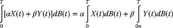
- Property 2. The integral of the indicator function of an interval I[a,b](t) = 1 when t ∈ [a, b], and zero otherwise, is just B(b) − B(a), 0 < a < b < T,
(3.220)
- Property 3. Zero mean property:
(3.221)

- Property 4. Isometry property:
(3.222)
The definition of the Ito integral may be extended to processes X(t) that may be approximated by sequences en of simple processes in the sense that

as n → ∞. In that case, one defines
In this definition, the limit does not depend on the approximating sequence. Also, the integral that arises this way satisfies Properties 1–4.
Now that one has defined the Ito integral of simple processes, one may define the Ito integrals of other processes. It may be shown that if a general predictable process satisfies certain conditions, the general process is a limit in probability of simple predictable processes discussed earlier. The Ito integral of general predictable processes is defined as a limit of integrals of simple processes. If X(t) is a predictable process such that

then the Ito integral

is defined and satisfies the above four properties.
For example, to undertake the integral

one may let 0 = t0 < t1 < t2 <![]() < tn = T be a partition of [0, T], then
< tn = T be a partition of [0, T], then
Then, for any n, en(t) is a simple process. One may take a sequence of the partitions such that maxi(ti+1 − ti) → 0 as n → ∞. The Ito integral of this simple function is given by

One may show that this sequence of integrals converges in probability and identify the limit. Adding and subtracting B2(ti+1), one obtains
and

since the first sum is a telescopic sum. Notice that from property 5 of Brownian motion path, the second sum converges to the limit T. Therefore, ![]() converges, and the limit is
converges, and the limit is

This example illustrates the difference between deterministic calculus and stochastic calculus. The quadratic variation of continuous functions, x(t), of finite variation in standard calculus is 0. Therefore, if one were calculating the integral of ![]() the same way as above the term
the same way as above the term ![]() would to the limit 0. Thus, the integral
would to the limit 0. Thus, the integral ![]() equals (1/2)x2(T).
equals (1/2)x2(T).
Now consider the main tools of stochastic calculus: Ito's formula, which is the stochastic counterpart of the chain rule in Calculus. Recall that Brownian motion has quadratic variation on [0, t] equal to t, for any t. This also may be expressed as the following:

Using this property and applying Taylor's formula, Ito's formula states that if f(x) is a twice-differentiable function, then for any t

and Ito's formula in differential notation becomes
The Ito Process
Next, one defines an Ito process: Let Y(t) be an Ito integral, defined as

Then, an Ito process is an Ito integral plus an adapted continuous process of finite variation. A process Y is called an Ito Process if for any 0 ≤ t ≤ T it can be represented as

More generally, if Y is an Ito process represented above, then it has a stochastic differential on [0, T] given by
for 0 ≤ t ≤ T. The function µ is often called the drift coefficient and the function σ is called the diffusion coefficient—terms inherited from studies in mass and energy transfers in areas within classical physics and engineering.
One last important case to consider is for functions of the form f {X(t), t}. If f(x, t) is a twice continuously differentiable function in x, as well as continuously differentiable in t, and X(t) represents an Ito process, then
This case of Ito's formula may be used to compute the Black–Scholes partial differential equation in the next section.
Derivation of the Black–Scholes Equation
Here, the price of a derivative security, V(S, t), will be derived. The model for a stock derived previously satisfies an Ito process defined in (3.237).
Therefore, one may let the function V(S, t) be twice differentiable in S and differentiable in t. Applying (3.238) one has
Substituting into (3.239) for dS with (3.210), one has
This simplifies to
Now set up a portfolio long one option, V, and short an amount (∂V/∂S) stock. Note from above that this portfolio is hedged. The value of this portfolio, π, is
The change dπ in the value of this portfolio over a small time interval dt is given by
Now substituting (Equations 3.241) and (3.210):
into Equation (3.243) for dV and dS one obtains
This simplifies to
It is important to note that this portfolio is completely risk-free because it does not contain the random Brownian motion term. Since this portfolio contains no risk it must earn the same as other short-term risk-free securities. If it earned more than this, arbitrageurs could make a profit by shorting the risk-free securities and using the proceeds to buy this portfolio. If the portfolio earned less arbitrageurs could make a riskless profit by shorting the portfolio and buying the risk-free securities. It follows for a riskless portfolio that
where r is the risk-free interest rate. Substituting for dπ and π from (3.245) and (3.242) yields
Further simplification yields the Black–Scholes differential equation:
Solution for a European Call
To solve the Black–Scholes equation, consider final and boundary conditions, or else the partial differential equation does not have a unique solution. As an illustration, a European call, C(S, t), will be solved given the exercise price E and the expiry date T.
The final condition at time t = T may be derived from the definition of a call option. If at expiration S > E the call option will be worth S − E because the buyer of the option can buy the stock for E and immediately sell it for S. If at expiration S < E the option will not be exercised and it will expire worthless. At t = T, the value of the option is known for certain to be the payoff:
This is the final condition for the differential equation.
In order to find boundary conditions, one considers the value of C when S = 0 and as S → ∞. If S = 0, then it is easy to see from (3.210) that dS = 0, and therefore S will never change. If at expiry S = 0, from (3.249) the payoff must be 0. Consequently, when S = 0 one has
Now when S → ∞, it becomes more and more likely the option will be exercised and the payoff will be (S – E). The exercise price becomes less and less important as S → ∞, so the value of the option is equivalent to
In order to solve the Black–Scholes equation, one needs to transform the equation into an equation one can work with. The first step is to eliminate of the S and S2 terms in (3.248) (16). To do this, consider the change of variables:
Using the chain rule from Calculus for transforming partial derivatives for functions of two variables, we have
Looking at (3.252)–(3.254), it may be shown that
Plugging these into (3.255) and (3.256) yields
Substituting (3.255)–(3.260) into the Black–Scholes partial differential equation gives the differential equation:
where
The initial condition C(S, T) = max(S − E, 0) is transformed into
Now we apply another change of variable and let
Then by simple differentiation, one has
Substituting these partials into (3.261) yields
We may eliminate the u terms and the ∂u/∂x terms by carefully choosing values of α and β such that
and
One may then rearrange these equations, so they can be written
We now have the transformation from v to u to be
resulting in the simple diffusion equation
The initial condition has now been changed as well to
The solution to the simple diffusion equation obtained above is well known to be
where u0(x, 0) is given by (3.274). In order to solve this integral, it is convenient to make a change of variable as follows:
so that
Substituting our initial condition into this equation results in
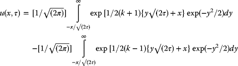
In order to solve this, one will solve each integral separately. The first integral can be solved by completing the square in the exponent. The exponent of the first integral is ![]() .
.
Factoring out the −1/2 gives us ![]() .
.
Separating out the term that is not a function of y, and adding and subtracting terms to set up a perfect square yields
which may be written as
and simplified to
Thus, the first integral reduces to
Now substituting
results in
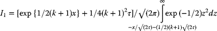
where
and
is the cumulative distribution function for the normal distribution.
The calculation of the second integral I2 is identical to that of I1, except that (k−1) replaces (k+1) throughout. Finally, one works the way backward with
and then substituting the inverse transformations
one finally obtains the desired result:
where
and
Conclusion
Note that in the derivation of the Black–Scholes differential equation, it was never restricted to a specific type of derivative security when trying to find the price for until the boundary conditions are specified for a European call. This means that a person can use the Black–Scholes differential equation to solve for the price of any type of option—by changing the boundary conditions only.
The Black–Scholes model revolutionized the world of finance. For the first time the model has given traders, hedgers, and investors a standard way to value options. The model has also caused a huge growth in the importance of financial engineering in the world of finance. Today, mathematicians are building models to maximize portfolio returns while minimizing risk. They are also building sophisticated computer programs to search for inefficiencies in the market. The world of finance is being built on mathematics and the Black–Scholes model was the beginning of this mathematical revolution.
3.8 Some Worked Examples
In the R domain:
R version 3.2.2 (2015-08-14) -- "Fire Safety"Copyright (C) 2015 The R Foundation for Statistical ComputingPlatform: i386-w64-mingw32/i386 (32-bit)R is free software and comes with ABSOLUTELY NO WARRANTY.You are welcome to redistribute it under certain conditions.Type 'license()' or 'licence()' for distribution details.Natural language support but running in an English localeR is a collaborative project with many contributors.Type 'contributors()' for more information and'citation()' on how to cite R or R packages in publications.Type 'demo()' for some demos, 'help()' for on-line help, or'help.start()' for an HTML browser interface to help.Type 'q()' to quit R.>> install.packages("Dowd")Installing package into ‘C:/Users/Bert/Documents/R/win-library/3.2’(as ‘lib’ is unspecified)--- Please select a CRAN mirror for use in this session ---# A CRAN mirror is selectedalso installing the dependencies ‘stringi’, ‘magrittr’, ‘stringr’, ‘RColorBrewer’, ‘dichromat’, ‘munsell’, ‘labeling’, ‘quadprog’, ‘digest’, ‘gtable’, ‘plyr’, ‘reshape2’, ‘scales’, ‘zoo’, ‘timeDate’, ‘tseries’, ‘fracdiff’, ‘Rcpp’, ‘colorspace’, ‘ggplot2’, ‘RcppArmadillo’, ‘bootstrap’, ‘forecast’There is a binary version available but the source version is later:binary source needs_compilationcolorspace 1.2-6 1.2-7 TRUEBinaries will be installedtrying URL 'https://cran.cnr.berkeley.edu/bin/windows/contrib/3.2/stringi_1.1.2.zip'Content type 'application/zip' length 14229497 bytes (13.6 MB)downloaded 13.6 MBtrying URL 'https://cran.cnr.berkeley.edu/bin/windows/contrib/3.2/magrittr_1.5.zip'Content type 'application/zip' length 149966 bytes (146 KB)downloaded 146 KBtrying URL 'https://cran.cnr.berkeley.edu/bin/windows/contrib/3.2/stringr_1.1.0.zip'Content type 'application/zip' length 119831 bytes (117 KB)downloaded 117 KBtrying URL 'https://cran.cnr.berkeley.edu/bin/windows/contrib/3.2/RColorBrewer_1.1-2.zip'Content type 'application/zip' length 26734 bytes (26 KB)downloaded 26 KBtrying URL 'https://cran.cnr.berkeley.edu/bin/windows/contrib/3.2/dichromat_2.0-0.zip'Content type 'application/zip' length 147767 bytes (144 KB)downloaded 144 KBtrying URL 'https://cran.cnr.berkeley.edu/bin/windows/contrib/3.2/munsell_0.4.3.zip'Content type 'application/zip' length 134334 bytes (131 KB)downloaded 131 KBtrying URL 'https://cran.cnr.berkeley.edu/bin/windows/contrib/3.2/labeling_0.3.zip'Content type 'application/zip' length 40854 bytes (39 KB)downloaded 39 KBtrying URL 'https://cran.cnr.berkeley.edu/bin/windows/contrib/3.2/quadprog_1.5-5.zip'Content type 'application/zip' length 51794 bytes (50 KB)downloaded 50 KBtrying URL 'https://cran.cnr.berkeley.edu/bin/windows/contrib/3.2/digest_0.6.10.zip'Content type 'application/zip' length 172481 bytes (168 KB)downloaded 168 KBtrying URL 'https://cran.cnr.berkeley.edu/bin/windows/contrib/3.2/gtable_0.2.0.zip'Content type 'application/zip' length 57917 bytes (56 KB)downloaded 56 KBtrying URL 'https://cran.cnr.berkeley.edu/bin/windows/contrib/3.2/plyr_1.8.4.zip'Content type 'application/zip' length 1119520 bytes (1.1 MB)downloaded 1.1 MBtrying URL 'https://cran.cnr.berkeley.edu/bin/windows/contrib/3.2/reshape2_1.4.1.zip'Content type 'application/zip' length 505413 bytes (493 KB)downloaded 493 KBtrying URL 'https://cran.cnr.berkeley.edu/bin/windows/contrib/3.2/scales_0.4.0.zip'Content type 'application/zip' length 604312 bytes (590 KB)downloaded 590 KBtrying URL 'https://cran.cnr.berkeley.edu/bin/windows/contrib/3.2/zoo_1.7-13.zip'Content type 'application/zip' length 900652 bytes (879 KB)downloaded 879 KBtrying URL 'https://cran.cnr.berkeley.edu/bin/windows/contrib/3.2/timeDate_3012.100.zip'Content type 'application/zip' length 791098 bytes (772 KB)downloaded 772 KBtrying URL 'https://cran.cnr.berkeley.edu/bin/windows/contrib/3.2/tseries_0.10-35.zip'Content type 'application/zip' length 321523 bytes (313 KB)downloaded 313 KBtrying URL 'https://cran.cnr.berkeley.edu/bin/windows/contrib/3.2/fracdiff_1.4-2.zip'Content type 'application/zip' length 106748 bytes (104 KB)downloaded 104 KBtrying URL 'https://cran.cnr.berkeley.edu/bin/windows/contrib/3.2/Rcpp_0.12.7.zip'Content type 'application/zip' length 3230471 bytes (3.1 MB)downloaded 3.1 MBtrying URL 'https://cran.cnr.berkeley.edu/bin/windows/contrib/3.2/colorspace_1.2-6.zip'Content type 'application/zip' length 391490 bytes (382 KB)downloaded 382 KBtrying URL 'https://cran.cnr.berkeley.edu/bin/windows/contrib/3.2/ggplot2_2.1.0.zip'Content type 'application/zip' length 2001613 bytes (1.9 MB)downloaded 1.9 MBtrying URL 'https://cran.cnr.berkeley.edu/bin/windows/contrib/3.2/RcppArmadillo_0.7.400.2.0.zip'Content type 'application/zip' length 1745518 bytes (1.7 MB)downloaded 1.7 MBtrying URL 'https://cran.cnr.berkeley.edu/bin/windows/contrib/3.2/bootstrap_2015.2.zip'Content type 'application/zip' length 104944 bytes (102 KB)downloaded 102 KBtrying URL 'https://cran.cnr.berkeley.edu/bin/windows/contrib/3.2/forecast_7.2.zip'Content type 'application/zip' length 1388535 bytes (1.3 MB)downloaded 1.3 MBtrying URL 'https://cran.cnr.berkeley.edu/bin/windows/contrib/3.2/Dowd_0.12.zip'Content type 'application/zip' length 396919 bytes (387 KB)downloaded 387 KBpackage ‘stringi’ successfully unpacked and MD5 sums checkedpackage ‘magrittr’ successfully unpacked and MD5 sums checkedpackage ‘stringr’ successfully unpacked and MD5 sums checkedpackage ‘RColorBrewer’ successfully unpacked and MD5 sums checkedpackage ‘dichromat’ successfully unpacked and MD5 sums checkedpackage ‘munsell’ successfully unpacked and MD5 sums checkedpackage ‘labeling’ successfully unpacked and MD5 sums checkedpackage ‘quadprog’ successfully unpacked and MD5 sums checkedpackage ‘digest’ successfully unpacked and MD5 sums checkedpackage ‘gtable’ successfully unpacked and MD5 sums checkedpackage ‘plyr’ successfully unpacked and MD5 sums checkedpackage ‘reshape2’ successfully unpacked and MD5 sums checkedpackage ‘scales’ successfully unpacked and MD5 sums checkedpackage ‘zoo’ successfully unpacked and MD5 sums checkedpackage ‘timeDate’ successfully unpacked and MD5 sums checkedpackage ‘tseries’ successfully unpacked and MD5 sums checkedpackage ‘fracdiff’ successfully unpacked and MD5 sums checkedpackage ‘Rcpp’ successfully unpacked and MD5 sums checkedpackage ‘colorspace’ successfully unpacked and MD5 sums checkedpackage ‘ggplot2’ successfully unpacked and MD5 sums checkedpackage ‘RcppArmadillo’ successfully unpacked and MD5 sums checkedpackage ‘bootstrap’ successfully unpacked and MD5 sums checkedpackage ‘forecast’ successfully unpacked and MD5 sums checkedpackage ‘Dowd’ successfully unpacked and MD5 sums checkedThe downloaded binary packages are inC:UsersBertAppDataLocalTempRtmp2n3pwvdownloaded_ packages> library(Dowd)Loading required package: bootstrapLoading required package: MASSLoading required package: forecastLoading required package: zooAttaching package: ‘zoo’The following objects are masked from ‘package:base’:as.Date, as.Date.numericLoading required package: timeDateThis is forecast 7.2Warning messages:1: package ‘Dowd’ was built under R version 3.2.52: package ‘bootstrap’ was built under R version 3.2.53: package ‘forecast’ was built under R version 3.2.54: package ‘zoo’ was built under R version 3.2.55: package ‘timeDate’ was built under R version 3.2.5> ls("package:Dowd")[1] "AdjustedNormalESHotspots"[2] "AdjustedNormalVaRHotspots"[3] "AdjustedVarianceCovarianceES"[4] "AdjustedVarianceCovarianceVaR"[5] "ADTestStat"[6] "AmericanPutESBinomial"[7] "AmericanPutESSim"[8] "AmericanPutPriceBinomial"[9] "AmericanPutVaRBinomial"[10] "BinomialBacktest"[11] "BlackScholesCallESSim"[12] "BlackScholesCallPrice"[13] "BlackScholesPutESSim"[14] "BlackScholesPutPrice"[15] "BlancoIhleBacktest"[16] "BootstrapES"[17] "BootstrapESConfInterval"[18] "BootstrapESFigure"[19] "BootstrapVaR"[20] "BootstrapVaRConfInterval"[21] "BootstrapVaRFigure"[22] "BoxCoxES"[23] "BoxCoxVaR"[24] "CdfOfSumUsingGaussianCopula"[25] "CdfOfSumUsingGumbelCopula"[26] "CdfOfSumUsingProductCopula"[27] "ChristoffersenBacktestForIndependence"[28] "ChristoffersenBacktestForUnconditionalCoverage"[29] "CornishFisherES"[30] "CornishFisherVaR"[31] "DBPensionVaR"[32] "DCPensionVaR"[33] "DefaultRiskyBondVaR"[34] "FilterStrategyLogNormalVaR"[35] "FrechetES"[36] "FrechetESPlot2DCl"[37] "FrechetVaR"[38] "FrechetVaRPlot2DCl"[39] "GaussianCopulaVaR"[40] "GParetoES"[41] "GParetoMEFPlot"[42] "GParetoMultipleMEFPlot"[43] "GParetoVaR"[44] "GumbelCopulaVaR"[45] "GumbelES"[46] "GumbelESPlot2DCl"[47] "GumbelVaR"[48] "GumbelVaRPlot2DCl"[49] "HillEstimator"[50] "HillPlot"[51] "HillQuantileEstimator"[52] "HSES"[53] "HSESDFPerc"[54] "HSESFigure"[55] "HSESPlot2DCl"[56] "HSVaR"[57] "HSVaRDFPerc"[58] "HSVaRESPlot2DCl"[59] "HSVaRFigure"[60] "HSVaRPlot2DCl"[61] "InsuranceVaR"[62] "InsuranceVaRES"[63] "JarqueBeraBacktest"[64] "KernelESBoxKernel"[65] "KernelESEpanechinikovKernel"[66] "KernelESNormalKernel"[67] "KernelESTriangleKernel"[68] "KernelVaRBoxKernel"[69] "KernelVaREpanechinikovKernel"[70] "KernelVaRNormalKernel"[71] "KernelVaRTriangleKernel"[72] "KSTestStat"[73] "KuiperTestStat"[74] "LogNormalES"[75] "LogNormalESDFPerc"[76] "LogNormalESFigure"[77] "LogNormalESPlot2DCL"[78] "LogNormalESPlot2DHP"[79] "LogNormalESPlot3D"[80] "LogNormalVaR"[81] "LogNormalVaRDFPerc"[82] "LogNormalVaRETLPlot2DCL"[83] "LogNormalVaRFigure"[84] "LogNormalVaRPlot2DCL"[85] "LogNormalVaRPlot2DHP"[86] "LogNormalVaRPlot3D"[87] "LogtES"[88] "LogtESDFPerc"[89] "LogtESPlot2DCL"[90] "LogtESPlot2DHP"[91] "LogtESPlot3D"[92] "LogtVaR"[93] "LogtVaRDFPerc"[94] "LogtVaRPlot2DCL"[95] "LogtVaRPlot2DHP"[96] "LogtVaRPlot3D"[97] "LongBlackScholesCallVaR"[98] "LongBlackScholesPutVaR"[99] "LopezBacktest"[100] "MEFPlot"[101] "NormalES"[102] "NormalESConfidenceInterval"[103] "NormalESDFPerc"[104] "NormalESFigure"[105] "NormalESHotspots"[106] "NormalESPlot2DCL"[107] "NormalESPlot2DHP"[108] "NormalESPlot3D"[109] "NormalQQPlot"[110] "NormalQuantileStandardError"[111] "NormalSpectralRiskMeasure"[112] "NormalVaR"[113] "NormalVaRConfidenceInterval"[114] "NormalVaRDFPerc"[115] "NormalVaRFigure"[116] "NormalVaRHotspots"[117] "NormalVaRPlot2DCL"[118] "NormalVaRPlot2DHP"[119] "NormalVaRPlot3D"[120] "PCAES"[121] "PCAESPlot"[122] "PCAPrelim"[123] "PCAVaR"[124] "PCAVaRPlot"[125] "PickandsEstimator"[126] "PickandsPlot"[127] "ProductCopulaVaR"[128] "ShortBlackScholesCallVaR"[129] "ShortBlackScholesPutVaR"[130] "StopLossLogNormalVaR"[131] "tES"[132] "tESDFPerc"[133] "tESFigure"[134] "tESPlot2DCL"[135] "tESPlot2DHP"[136] "tESPlot3D"[137] "TQQPlot"[138] "tQuantileStandardError"[139] "tVaR"[140] "tVaRDFPerc"[141] "tVaRESPlot2DCL"[142] "tVaRFigure"[143] "tVaRPlot2DCL"[144] "tVaRPlot2DHP"[145] "tVaRPlot3D"[146] "VarianceCovarianceES"[147] "VarianceCovarianceVaR">> # Market Risk of American Put with given parameters.> AmericanPutESBinomial(0.20, 27.2, 25, .16, .05, 60, 20, .95,+ 30)> # Outputting:[1] 0.2> # The ES (Expected Shortfall) of this American Put Option is 0.2.>
In the R domain:
>> # Estimates the price of an American Put> AmericanPutPriceBinomial(27.2, 25, .03, .2, 60, 30)> # Outputting:[1] 0.1413597> # The ES (Expected Shortfall) of this American Put Option is 0.1413597.>>
Review Questions and Exercises
- Contrast the following three classical theories of portfolio allocation using
- The Markowitz model,
- The Black–Litterman model, and
- Capital asset pricing model (CAPM)
in terms of the following aspects of these models:
- The assumptions of each model
- The advantages and disadvantages of these assumptions
- With respect to the Black–Litterman model for assets allocation and portfolio optimization,
- state and discuss the basic assumptions and the strengths and weaknesses of this model;
- state and discuss available improvements suggested for this model.
- The Black–Scholes equation, and boundary conditions, for a European option call is
where
C = the value of the call = C(S, t), S = the fixed Strike price, t = time, r = the risk-free interest rate, and
σ = the volatility of the underlying asset. (Equation RE-3.1) is a rather complicated second-order partial differential equation (pde).
It may be somewhat simplified, as follows:
If S is fixed and E is variable, show the European option price. C = C(E, t) also satisfies the following partial differential equation:
which may be considered as a simplified form of the Black–Scholes equation.
As an Example:
In the analysis of a pde, often useful solutions may be found by judicial changes of variables. A typical case is the classical heat/mass diffusion equation, solvable by the method of Separation of Variables:
(RE-3.3)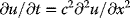
with boundary conditions:

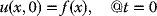
and an initial condition: u(x, 0) = f(x), a given function of x.
An elementary approach is to assume the separable of the independent variables: x and t, so that one may write
and obtain, after some elementary steps, the final solution:
where

- The CRAN package BLCOP—implementing the Black–Litterman approach to Assets Allocation and Portfolio Optimization:
BLCOP: Black–Litterman and Copula Opinion Pooling Frameworks
An implementation of the Black–Litterman model and Atilio Meucci's copula opinion pooling framework.da
Version: 0.3.1 Depends: methods, MASS, quadprog Imports: RUnit (≥ 0.4.22), timeSeries, fBasics, fMultivar, fPortfolio (≥3011.81) Suggests: sn, corpcor, mnormt Published: 2015-02-04 Author: Francisco Gochez, Richard Chandler-Mant, Suchen Jin, Jinjing Xie Maintainer: Ava Yang <ayang at mango-solutions.com> License: GPL-3 NeedsCompilation: no Materials: NEWS CRAN checks: BLCOP results Downloads:
Run the following example in the R domain:
optimalPortfolios
Calculates Optimal Portfolios under Prior and Posterior Distributions
Description
These are wrapper functions that calculate optimal portfolios under the prior and posterior return distributions. optimalPortfolios works with a user-supplied optimization function, although simple Markowitz minimum-risk optimization is done with solve. QP from quadprog if none is supplied.
optimalPortfolios.fPort is a generic utility function that calculates optimal portfolios using routines from the fPortfolio package.
Usage
optimalPortfolios(result, optimizer = .optimalWeights.simpleMV,..., doPlot = TRUE, beside = TRUE)optimalPortfolios.fPort(result, spec = NULL,constraints = "LongOnly",optimizer = "minriskPortfolio",inputData = NULL,numSimulations = BLCOPOptions("numSimulations"))Arguments
result An object of class BL Result. optimiser For optimalPortfolios, an optimization function. It should take as arguments a vector of means and a variance–covariance matrix, and should return a vector of optimal weights. For optimalPortfolios, the name of a fPortfolio function that performs portfolio optimization. spec Object of class fPORTFOLIOSPEC. If NULL, will use a basic mean-variance spec for Black–Litterman results, and a basic CVaR spec for COP results. inputData Time series data (any form that can be coerced into a timeSeries object). constraints String of constraints that may be passed into fPortfolio optimization routines. numSimulations For COP results only—the number of posterior simulations to use in the optimization (large numbers here will likely cause the routine to fail). ... Additional arguments to the optimization function. doPlot A logical flag. Should barplots of the optimal portfolio weights be produced? beside A logical flag. If a barplot is generated, should the bars appear side-by side? If FALSE, differences of weights will be plotted instead. Details
By default, optimizer is a simple function that performs Markowitz optimization via solve.QP. In addition to a mean and variance, it takes an optional constraints parameter that if supplied should hold a named list with all of the parameters that solve.QP takes.
Value
optimalPortfolios Will return a list with the following items. priorPFolioWeights The optimal weights under the prior distribution. postPFolioWeights The optimal weights under the posterior distribution. optimalPortfolios.f Port Will return a similar list with two elements of class fPORTFOLIO. Note
It is expected that optimalPortfolios will be deprecated in future releases in favor of optimalPortfolios.fPort.
Author(s)
Francisco Gochez <[email protected]>
Examples
entries <- c(0.001005, 0.001328, -0.000579,-0.000675, 0.000121, 0.000128,-0.000445, -0.000437, 0.001328, 0.007277, -0.001307, -0.000610,-0.002237, -0.000989, 0.001442,-0.001535, -0.000579,-0.001307,0.059852, 0.027588, 0.063497, 0.023036, 0.032967, 0.048039,-0.000675, -0.000610, 0.027588, 0.029609, 0.026572, 0.021465,0.020697, 0.029854, 0.000121,-0.002237, 0.063497, 0.026572,0.102488, 0.042744, 0.039943, 0.065994, 0.000128,-0.000989,0.023036, 0.021465, 0.042744, 0.032056, 0.019881, 0.032235,-0.000445, 0.001442, 0.032967, 0.020697, 0.039943, 0.019881,0.028355, 0.035064, -0.000437, -0.001535, 0.048039, 0.029854,0.065994, 0.032235, 0.035064, 0.079958)varcov <- matrix(entries, ncol = 8, nrow = 8)mu <- c(0.08, 0.67,6.41, 4.08, 7.43, 3.70, 4.80, 6.60) / 100pick <- matrix(0, ncol = 8, nrow = 3, dimnames = list(NULL,letters[1:8]))pick[1,7] <- 1pick[2,1] <- -1; pick[2,2] <- 1pick[3, 3:6] <- c(0.9, -0.9, .1, -.1)confidences <- 1 / c(0.00709, 0.000141, 0.000866)views <- BLViews(pick, c(0.0525, 0.0025, 0.02), confidences,letters[1:8])posterior <- posteriorEst(views, tau = 0.025, mu, varcov)optimalPortfolios(posterior, doPlot = TRUE)optimalPortfolios.fPort(posterior, optimizer = "tangencyPortfolio")# An example based on one found in "Beyond Black-Litterman:# Views on Non-normal Markets"dispersion <-c(.376,.253,.360,.333,.360,.600,.397,.396,.578,.775) / 1000sigma <- BLCOP:::.symmetricMatrix(dispersion, dim = 4)caps <- rep(1/4, 4)mu <- 2.5 * sigmadim(mu) <- NULLmarketDistribution <- mvdistribution("mt", mean = mu, S =sigma, df = 5)pick <- matrix(0, ncol = 4, nrow = 1, dimnames = list(NULL,c("SP", "FTSE", "CAC", "DAX")))pick[1,4] <- 1vdist <- list(distribution("unif", min = -0.02, max = 0))views <- COPViews(pick, vdist, 0.2, c("SP", "FTSE", "CAC","DAX"))posterior <- COPPosterior(marketDistribution, views)optimalPortfolios.fPort(myPosterior, spec = NULL, optimizer ="minriskPortfolio",inputData = NULL, numSimulations = 100)## End - The CRAN package PerformanceAnalytics—providing a number of useful programs for investment risk analysis and portfolio performance.
Package ‘PerformanceAnalytics’ February 19, 2015 Type Package Title Econometric tools for performance and risk analysis Version 1.4.3541 Date 2014-09-15 04:39:58–0500 (Mon, Sep 15, 2014) Description Collection of econometric functions for performance and risk analysis. This package aims to aid practitioners and researchers in utilizing the latest research in analysis of nonnormal return streams. In general, it is most tested on return (rather than price) data on a regular scale, but most functions will work with irregular return data as well, and increasing numbers of functions will work with P&L or price data where possible Imports zoo Depends R (>= 3.0.0), xts (>= 0.9) Suggests Hmisc, MASS, quantmod, gamlss, gamlss.dist, robustbase, quantreg, gplots License GPL-2 | GPL-3 URL http://r-forge.r-project.org/projects/returnanalytics/ Copyright (c) 2004–2014 Authors Brian G. Peterson [cre, aut, cph], Peter Carl [aut, cph], Kris Boudt [ctb, cph], Ross Bennett [ctb], Joshua Ulrich [ctb], Eric Zivot [ctb], Matthieu Lestel [ctb], Kyle Balkissoon [ctb], Diethelm Wuertz [ctb] Maintainer Brian G. Peterson <[email protected]> Needs Compilation yes Repository CRAN Date/Publication 2014-09-16 09:47:58 ****chart.TimeSeries Creates a time series chart with some extensions.DescriptionDraws a line chart and labels the x-axis with the appropriate dates. This is really a “primitive”, sinceit extends the base plot and standardizes the elements of a chart. Adds attributes for shading areasof the timeline or aligning vertical lines along the timeline. This function is intended to be usedinside other charting functions.Usagechart.TimeSeries(R, auto.grid = TRUE, xaxis = TRUE, yaxis = TRUE,yaxis.right = FALSE, type = “l”, lty = 1, lwd = 2, las = par(“las”),main = NULL, ylab = NULL, xlab = "", date.format.in = “%Y-%m-%d”,date.format = NULL, xlim = NULL, ylim = NULL,element.color = “darkgray”, event.lines = NULL, event.labels = NULL,period.areas = NULL, event.color = “darkgray”,period.color = “aliceblue”, colorset = (1:12), pch = (1:12),legend.loc = NULL, ylog = FALSE, cex.axis = 0.8, cex.legend = 0.8,cex.lab = 1, cex.labels = 0.8, cex.main = 1, major.ticks = “auto”,minor.ticks = TRUE, grid.color = “lightgray”, grid.lty = “dotted”,xaxis.labels = NULL, ...)charts.TimeSeries(R, space = 0, main = “Returns”, ...)ArgumentsR an xts, vector, matrix, data frame, timeSeries or zoo object of asset returnsauto.grid if true, draws a grid aligned with the points on the x and y axesxaxis if true, draws the x axisyaxis if true, draws the y axisyaxis.right if true, draws the y axis on the right-hand side of the plottype set the chart type, same as in plotlty set the line type, same as in plotlwd set the line width, same as in plotlas set the axis label rotation, same as in plotmain set the chart title, same as in plotylab set the y-axis label, same as in plotxlab set the x-axis label, same as in plotdate.format.in allows specification of other date formats in the data object, defaults to “%Y-%m-%d”date.format re-format the dates for the xaxis; the default is “%m/%y”chart.TimeSeries 73xlim set the x-axis limit, same as in plotylim set the y-axis limit, same as in plotelement.color provides the color for drawing chart elements, such as the box lines, axis lines,etc. Default is “darkgray”event.lines If not null, vertical lines will be drawn to indicate that an event happened duringthat time period. event.lines should be a list of dates (e.g., c(“09/03”,“05/06”))formatted the same as date.format. This function matches the re-formatted rownames (dates) with the events.list, so to get a match the formatting needs to becorrect.event.labels if not null and event.lines is not null, this will apply a list of text labels (e.g.,c(“This Event”, “That Event”) to the vertical lines drawn. See the examplebelow.period.areas these are shaded areas described by start and end dates in a vector of xts daterangees, e.g., c(“1926-10::1927-11”,“1929-08::1933-03”) See the examplesbelow.event.color draws the event described in event.labels in the color specifiedperiod.color draws the shaded region described by period.areas in the color specifiedcolorset color palette to use, set by default to rational choicespch symbols to use, see also plotlegend.loc places a legend into one of nine locations on the chart: bottomright, bottom,bottomleft, left, topleft, top, topright, right, or center.ylog TRUE/FALSE set the y-axis to logarithmic scale, similar to plot, default FALSEcex.axis The magnification to be used for axis annotation relative to the current settingof ‘cex’, same as in plot.cex.legend The magnification to be used for sizing the legend relative to the current settingof ‘cex’.cex.lab The magnification to be used for x- and y-axis labels relative to the currentsetting of ‘cex’.cex.labels The magnification to be used for event line labels relative to the current settingof ‘cex’.cex.main The magnification to be used for the chart title relative to the current setting of‘cex’.major.ticks Should major tickmarks be drawn and labeled, default ‘auto’minor.ticks Should minor tickmarks be drawn, default TRUEgrid.color sets the color for the reference gridgrid.lty defines the line type for the gridxaxis.labels Allows for non-date labeling of date axes, default is NULLspace default 0... any other passthru parametersAuthor(s)Peter Carl74 chart.TimeSeriesSee Alsoplot, par, axTicksByTimeExamples# These are start and end dates, formatted as xts ranges.## http://www.nber.org-cycles.htmlcycles.dates<-c(“1857-06/1858-12”,"1860Examples# These are start and end dates, formatted as xts ranges.## http://www.nber.org-cycles.htmlcycles.dates<-c(“1857-06/1858-12”,“1860-10/1861-06”,“1865-04/1867-12”,“1869-06/1870-12”,“1873-10/1879-03”,“1882-03/1885-05”,“1887-03/1888-04”,“1890-07/1891-05”,“1893-01/1894-06”,“1895-12/1897-06”,“1899-06/1900-12”,“1902-09/1904-08”,“1907-05/1908-06”,“1910-01/1912-01”,“1913-01/1914-12”,“1918-08/1919-03”,“1920-01/1921-07”,“1923-05/1924-07”,“1926-10/1927-11”,“1929-08/1933-03”,“1937-05/1938-06”,“1945-02/1945-10”,“1948-11/1949-10”,“1953-07/1954-05”,“1957-08/1958-04”,“1960-04/1961-02”,“1969-12/1970-11”,“1973-11/1975-03”,“1980-01/1980-07”,“1981-07/1982-11”,“1990-07/1991-03”,“2001-03/2001-11”,“2007-12/2009-06”)# Event lists - FOR BEST RESULTS, KEEP THESE DATES IN ORDERrisk.dates = c(“Oct 87”,“Feb 94”,“Jul 97”,“Aug 98”,“Oct 98”,“Jul 00”,“Sep 01”)risk.labels = c(“Black Monday”,chart.VaRSensitivity 75“Bond Crash”,“Asian Crisis”,“Russian Crisis”,“LTCM”,“Tech Bubble”,“Sept 11”)data(edhec)R=edhec[,“Funds of Funds”,drop=FALSE]Return.cumulative = cumprod(1+R) - 1chart.TimeSeries(Return.cumulative)chart.TimeSeries(Return.cumulative, colorset = “darkblue”,legend.loc = “bottomright”,period.areas = cycles.dates,period.color = “lightblue”,event.lines = risk.dates,event.labels = risk.labels,event.color = “red”, lwd = 2)
Solutions to Exercise 3: The Black-Scholes Equation
3. For the Black–Scholes (equation RE-3.1),
Let
for some function f, then
Apply the change of variables stated in (RE-3.5) to reduce the Black–Scholes (equation RE-3.1) to its simpler form:
which is (RE-3.2).
Proof:
Since ![]() , from (RE-3.5),
, from (RE-3.5),
therefore, upon substituting for f(S/E) from (RE-3.6):
Again, since ![]() , from (RE-3.5),
, from (RE-3.5),
Therefore,
or
Hence,
Again, from (RE-3.5),
Therefore,

Therefore,
upon substituting for C from (RE-3.5).
Also, from (RE-3.8),
Hence,
Now,
Hence,
which is an important intermediate result.
Similarly, it may be shown that
which is a final result that may be readily obtained as follows:
Since ![]() , from (RE-3.13)
, from (RE-3.13)
and
namely,
Moreover, since ![]() , from (RE-3.12)-->
, from (RE-3.12)-->![]() , from (RE-3.5)
, from (RE-3.5)
Therefore,
and
by the differentiation of a quotient rule or
Combining (RE-3.15) and (RE-3.17), one finally obtains (RE-3.14), as required.And now, upon substituting for the terms ![]() and S∂C/∂S, from (RE-3.14) and (RE-3.13), respectively, into the Black–Scholes (equation RE-3.1), the result is
and S∂C/∂S, from (RE-3.14) and (RE-3.13), respectively, into the Black–Scholes (equation RE-3.1), the result is
namely,
namely,
namely,
which is (RE-3.7), as required.