2
Probabilistic Calculus for Modeling Financial Engineering
2.1 Introduction to Financial Engineering
To establish useful and realistic mathematical models for financial analysis, with the objectives of assets allocation and the concomitant gains, or losses, it is useful to consider both discrete models and continuous models.
2.1.1 Some Classical Financial Data
Consider the following two typical sets of financial data:
- Dow Jones – 100 year historical chart (Figure 2.1)
Interactive chart of the Dow Jones Industrial Average (DJIA) stock market index for the last 100 years.
This historical data is inflation-adjusted using the headline CPI and each data point represents the month-end closing value. The current month is updated on an hourly basis with today's latest value. The current value of the DJIA as of 08:48 p.m. EDT on June 3, 2016 is $17,838.56.
- Apple, Inc., AAPL – 5-year historical prices (Figure 2.2)

Figure 2.1 Dow Jones Industrial Average (DJIA) –100 year historical chart.

Figure 2.2 Apple, Inc., AAPL (a 5-year historical prices).
2.2 Mathematical Modeling in Financial Engineering
2.2.1 A Discrete Model versus a Continuous Model
In general, a discrete model calls for analysis and solutions using finite difference techniques, whereas a continuous model, using partial and total derivatives, leads to a financial theory consisting of systems of partial differential equations, with total and partial derivatives. Such systems of differential equations benefit from the vast reservoir of support from the well-developed field of systems of total and partial differential equations.
An outstanding example is the vast mathematical literature developed, or being developed, for the Black–Scholes model for financial derivatives.
2.2.2 A Deterministic Model versus a Probabilistic Model
2.2.2.1 Calculus of the Deterministic Model
In deterministic calculus of functions, f(x), of a single variable x, there are some important results, commonly called theorems, available for relating the variability characteristics of such functions. These theorems include the following:
- The Mean Value Theorem:
If f(x) is continuous in the closed interval [a, b], and is differentiable in the open interval (a, b), then there is a value ξ of x, namely, a < ξ < b, such that
(2.1)
- The Higher Mean Value Theorems:
For 0 < θ < 1
(2.2)
If f′(x) is continuous for a ≤ x ≤ b, and if f″(x) exists for a < x < b, and if h =b – a, and 0 < θ2 < 1, then
(2.3)
- The General Mean Value Theorem (Taylor's Theorem):
If f(n−1)(x) is continuous for the closed interval a ≤ x ≤ b, and f(n)(x) exists for a < x < b, then
(2.4)
where a < ξ < b; and if b = a + h, then
The continuity of f(n−1)(x) involves that of f(x), f′(x), f″(x),…, f(n−2)(x).
- Taylor's Theorem for Functions of Several Variables:
Taylor's formula for functions of one variable, Equation (2.5), may be generalized to functions of several variables having continuous derivatives of order n in a given region of space. The following procedure is outlined for functions of two variables – the result has all the features of more general cases.
Let f(x, y) be a function of two variables (x, y) having continuous derivatives of order n in some region containing the point.

and let
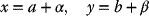
be a nearby point in the region. The equations of a straight line segment joining these two points may be expressed in the form
and, along this segment,
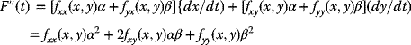
is a composite function of t having continuous derivatives of order n. Thus, F(t) may be represented by the Maclaurin formula:The successive derivatives of F(t) may be computed from Equation (2.7) and by the chain rule for differentiating composite functions:
If u = f(x, y), then
Thus,
where in the last step, one recalls Equation (2.6).
Similarly,
and
where Cn,r ≡ n!/[r! (n – r)!] are the binomial coefficients.
From Equation (2.6), it is seen that t = 0 corresponds to the point: x = a, y = b, so that
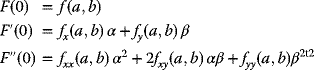
and so on.
Substituting these values in Equation (2.8) gives
where Rn = [F(n)(θt)/n!] tn, 0 < θ < 1.
Now, from Equation (2.6), αt = x − a and βt = y − b, so that Equation (2.11) takes the form

which is the Taylor formula (for two variables, in this case).
2.2.2.2 The Geometric Brownian Motion (GBM) Model and the Random Walk Model
Historically, the GBM had been developed in terms of the concept of the random walk, Wn(t), which has the following characteristics:
For a positive integer n, the binomial process Wn(t) may be defined by the following characteristic properties:
- Wn(t) = 0, at t = 0
- Wn(t) has layer spacing 1/n
- There exist up and down jumps, equal and of magnitude 1/√n
- Wn(t) has measure P, given by up and down probabilities ½ everywhere
Thus, if X1, X2, X3,…, Xi is a sequence of independent binomial random variables taking values +1 or −1 with equal probability, then the value of Wn at the ith step is
2.2.2.3 What Does a “Random Walk” Financial Theory Look Like?
The following chart is a simple example.
Random walk hypothesis test by increasing or decreasing the value of a fictitious stock based on the odd/even value of the decimals of π. The chart resembles a stock chart. (Figure 2.3)
Figure 2.3 An example of a random walk based on the odd/even value of the decimals of π = 3.14159. (Ordinates are arbitrary) (Available at https://en.wikipedia.org/wiki/Random_walk_hypothesis)
Remarks:
- A Brownian motion wanders randomly with zero mean, but a company stock usually grows at some rate (even if it just increases with normal inflation, etc.).
- Thus one may choose to add in a drift factor μ. For example, the random walk process may be described as
in which
- Wt is the log of the asset price at time t
- μ is a drift constant
- ∊t is a random disturbance term for which the exceptions
It had been demonstrated that the random walk hypothesis is inaccurate, there are trends in the stock market, and the stock market is somewhat predictable.
For progressing from a pure GBM to a modifiable deterministic–probabilistic model for the stock market, the following path may be followed:
- A deterministic model versus a probabilistic model
- A combined deterministic and probabilistic model
2.3 Building an Effective Financial Model from GBM via Probabilistic Calculus
The attractive characteristics of the GBM are quite powerful. They may be retained if some of its attractive features are retained in a more realistic environment, even if any such hybrid result is considerably complex. This may well be a worthwhile endeavor!
For any smooth, namely, differentiable, path, consider a small time segment, it is acceptable that this time segment consists of a continuous and differentiable function dft within this time slot dt such that
where μt is the slope or drift scaling function.
From this simple beginning, one may consider all other possible Newtonian functions. A likely possibility is one in which the drift μt may depend on the existing value of the function ft, namely,
2.3.1 A Probabilistic Model for the Stock Market
In a stock market that reflects a realistic probabilistic characteristic, the stock price Xt, at any time t, may be considered as one having both
- a Browning motion term σt dWt and
- a Newtonian characteristic term based upon dt: μt(Xt, t) dt,
so that the infinitesimal change of X may be represented by
in which
- the drift μt can depend on the time t,
- the drift μt can depend on the value of X and W, up to time t, and
- the noisiness or volatility, σt, of the process X can depend on the history of the process.
This approach, however, does provide a practical (though not universal) definition of a probabilistic process (sometimes known as a stochastic process).
2.3.2 Probabilistic Processes for the Stock Market Entities
A probabilistic process X is a continuous process such that

in which σ and μ are random processes such that ![]() is finite for all times t, with probability 1. The differential form of Equation (2.17) is
is finite for all times t, with probability 1. The differential form of Equation (2.17) is
2.3.3 Mathematical Modeling of Stock Prices
In modeling stock prices, it certainly should not escape ones attention that, in practice, a price can and may change at any instant, and not at some fixed times when a portfolio may be considered for rebalancing. Hence, these observations call for the requirements that
where both σt and μt depend on W, and Equation (2.18) may be written as
which is the probabilistic (or stochastic) differential equation ( PDE) for Xt.
As with any deterministic differential equation, a PDE
- need not have an explicit or implicit solution and
- if a solution should exist, it need not be unique.
Moreover, probabilistic differentials of systems whose volatility and drift depend not only on t and Xt, but also on other factors in the history of the system behavior.
2.3.4 A Simple Case
When σ and μ are both constants:
If X has constant volatility σ and drift μ, then the system PDE for X is
then (if X0 = 0) the corresponding solution is clearly
And, if the differential form of σ Wt may be assumed to be σ dWt, then it is seen that (Equation 2.20b) is the unique solution of (Equation 2.20a).
Nontrivial Cases: For a somewhat more complex case,
It seems that the solution to the Equation (2.21) is nontrivial.
2.4 A Continuous Financial Model Using Probabilistic Calculus: Stochastic Calculus, Ito Calculus
Deterministic Calculus
Probabilistic Calculus
For a continuous model representing the real-life market of financial entities such as stocks, bonds, derivatives, and so on, the following basic model characteristics should be included:
- The value of the entity can change at any time, and indeed, from moment to moment.
- The actual values may be expressed in arbitrarily small fractions in terms of a real number.
- The process changes continuously, and the value cannot make – abrupt – jumps. Thus, if the security values changes from 10 to 11, it must have passed through all the values in between, albeit quickly.
Historically, the motion of the stock price, variations with time, had been likened to one well-known physical process – that followed by a random movement of gas particles – namely, the geometric Brownian motion (GBM).
2.4.1 A Brief Observation of the Geometric Brownian Motion
Figure 2.4a shows two sample paths of GBM, with different parameters. The blue line has larger drift, the green line has larger variance.

Figure 2.4 (a) Geometric Brownian motion (See: Wikipedia).
A GBM may be considered as a continuous-time probabilistic motion in which the logarithm of the randomly varying quantity follows a Brownian motion (also known as a Wiener process) with drift. Thus, it is an important example of probabilistic processes satisfying a probabilistic differential equation. It is used in mathematical finance to model stock prices in the Black–Scholes model.
One may approach the solution of equations such as (2.20), in steps, now known as the Ito calculus, as follows:
2.4.2 Ito Calculus
Here one needs to establish the tools for solving a probabilistic (or stochastic) differential equation such as Equation (2.22)
to provide for steps similar tools developed for deterministic or Newtonian calculus: along the lines of integration by parts, the chain rule, the product rule, and so on.
2.4.2.1 The Ito Lemma
The Ito Lemma is named after its discoverer, the brilliant Japanese mathematician Prof. Dr. Kiyoshi Ito, who passed away on November 10, 2008, at the age of 93. His work created a field of mathematics that is a calculus of probabilistic, or stochastic, variables (http://www.sjsu.edu/faculty/watkins/ito.htm).
Changes in a variable, such as the price of a stock, involve two components:
- A deterministic component that is a function of time.
- A probabilistic, or stochastic, component that depends upon a random variable.
Let S be the stock price at time t, and let dS be the infinitesimal change in S over the infinitesimal interval of time dt. The change in the random variable z over this interval of time is dz. Hence, the change in stock price is given by
where a and b may be functions of S and t as well as other variables; that is,
The expected value of dz is zero, so the expected value of dS is equal to the deterministic component adt. Concomitantly, the random variable dz represents an accumulation of random contributions over the interval dt. Applying the central limit theorem, which implies that dz has a normal distribution and hence is completely characterized by its mean and standard deviation:
- The mean, or expected value, of dz is zero.
- The variance of a random variable that is the accumulation of independent effects over a given interval of time is proportional to the length of the interval: in this case dt. Hence, the standard deviation of dz is proportional to the square root of dt, namely, (dt)½.
All of this means that the random variable dz is equivalent to a random variable w(dt)½, where w is a standard normal variable with mean zero and standard deviation equal to unity.
Now consider another variable C, such as the price of a call option: it is a function of S and t, say C = f(S, t): because C is a function of the probabilistic variable S, it will have a probabilistic component S as well as a deterministic component. Thus, C will have a representation of the form
where the coefficients p and q may be functions of S, t, and possibly other variables; that is,
It remains to be determined how the functions p and q are related to the functions a and b in the equation
The answer may be found using the Ito Lemma:
Remark: The Ito Lemma is crucial in deriving differential equations for the value of derivative securities such as stock options.
A Proof of the Ito Lemma:
A derivation of the Ito Lemma is provided herein.
The Taylor series for f(S, t) gives the increment in C as

For example: The increment in stock price dS is given by
where w is a standard normal random variable and v is the scale of the variability of the random element; that is, its standard deviation. Substitution of adt +bvw(dt)½ for dS in Equation (2.27) yields
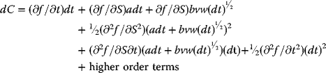
With the expansion of the squared term and the product term the result is
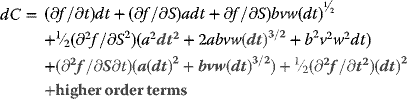
Taking into account the infinitesimal nature of dt so that dt to any power higher than unity vanishes, namely, all the terms in red in Equation (2.32) vanish, so that Equation (2.32) may be reduced to

Now, the expected value of w2 is unity, hence the expected value of dC is
This, (2.32), is the deterministic component of dC.
The probabilistic, or stochastic, component is the term that depends upon dz, which in (2.31) is represented as vw(dt)½. Therefore, the probabilistic, or stochastic, component is
In the foregoing derivation, it would seem that there is an additional stochastic term that arises from the random deviations of w2 from its expected value of 1; that is, the additional term
However, the variance of this additional term is proportional to (dt)2, whereas the variance of the stochastic term given in Equation (2.33) is proportional to (dt). Thus the stochastic term given in Equation (2.34) vanishes in comparison with the stochastic term given in Equation (2.33).
Remarks:
- The Ito Lemma Is Essential in the Derivation of the Black–Scholes Equation
An immediate question is whether Black–Scholes equation is an extension of Ito's Lemma for stable distributions of z other than the normal distribution. This question may be investigated in the study of stable distributions.
- Probabilistic (or Stochastic) Calculus and the Ito Lemma
Now, a probabilistic process St is a GBM if it satisfies the following probabilistic differential equation:
where Wt is the Wiener or Brownian motion, and μ the percentage drift and σ the percentage volatility are constants.
Here, μ is used to model deterministic behavior and σ is used to model a set of unpredictable events occurring during the motion.
- Solving the Probabilistic Differential Equation
For an arbitrary initial value S0 the above probabilistic differential Equation (2.37) has the analytic solution
(2.38)
This result may be obtained as follows:
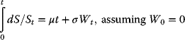
- First divide the probabilistic differential (Equation 2.37) by St in order to have the choice random variable on only one side.
- Next, write the equation in integral form (known as the Ito form):
(2.39)
- At this point, it might appear that dS/St may be related to ln St.
However, St is an Ito process, requiring the use of Ito Calculus.
Applying the Ito Lemma leads to
where dSt dSt is the quadratic variation of the SDE, which may be written as d[S]t or <S.>t. In this case, one has
- Substituting the value of dSt in Equation (2.41), and simplifying, one obtains
(2.42)

- Taking the exponential, and multiplying both sides by S0 gives the solution (2.40).
2.5 A Numerical Study of the Geometric Brownian Motion (GBM) Model and the Random Walk Model Using R
2.5.1 Modeling Real Financial Data
2.5.1.1 The Geometric Brownian Motion (GBM) Model and the Random Walk Model
Historically, the GBM had been developed in terms of the concept of the random walk, Wn(t), which has the following characteristics:
For a positive integer n, the binomial process Wn(t) may be defined by the following characteristic properties:
- Wn(t) = 0, at t = 0
- Wn(t) has layer spacing 1/n
- There exist up and down jumps, equal and of magnitude 1/√n
- Wn(t) has measure P, given by up and down probabilities ½ everywhere.
Thus, if X1, X2, X3,…, Xi is a sequence of independent binomial random variables taking values +1 or −1 with equal probability, then the value of Wn at the ith step is
What does a “Random Walk” look like?
The chart that follows is a simple example.
Random walk hypothesis test by increasing or decreasing the value of a fictitious stock based on the odd/even value of the decimals of π. The chart resembles a stock chart (Figure 2.5a).


Figure 2.5 (a) An example of a random walk based on the odd/even values of the decimals of π.
Notes:
- A Brownian motion wanders randomly with zero mean, but a company stock usually grows at some rate (even if it just increases with normal inflation).
- Thus one may choose to add in a drift factor. For example, the process with a constant noise factor σ may be represented by
(2.44)

- A Deterministic Model versus a Probabilistic Model
- A Combined Deterministic and Probabilistic Model
2.5.1.2 Other Models for Simulating Random Walk Systems Using R
The following are the two, among many, efficient models for simulating random walk systems that have been found to be useful in financial engineering and econometric data modeling:
- The Cox–Ingersoll–Ross (CIR) model
- The Chan–Karolyl– Longstaff–Sanders (CKLS) model
The CIR model is generally used to describe the evolution of interest rates. It is a type of “one-factor model” (aka a short rate model) as it models interest rate movements as driven by only one source of market risk. The model may be used in the valuation of interest rate derivatives. It was introduced in 1985 by J.C. Cox, J.E. Ingfersoll, and S.A. Ross. The CIR model assumes that the instantaneous interest rate follows the stochastic (probabilistic) differential equation. The CIR is an ergodic process, and possesses a stationary distribution.
The CKLS models belong to a class of parametric stochastic differential equations widely used in many finance applications, in particular to model interest rates or asset prices. This model nests a class of asset pricing models such as the CIR. This flexibility of the CKLS model spawns many empirical applications.
2.5.2 Some Typical Numerical Examples of Financial Data Using R
To demonstrate the GBM model as well as the random walk model, the R Program Sim.DiffProc, available from CRAN, is chosen. A typical worked example is selected, and the associated R program is run, outputting the associated numerical and graphical results:
| Package: | Sim.DiffProc |
| Type: | Package |
| Title: | Simulation of Diffusion Processes |
| Version: | 3.2 |
| Date: | February 9, 2016 |
| Author | A. C. Guidoum and K. Boukhetala |
| Maintainer | A. C. Guidoum <[email protected]> |
| Encoding | UTF-8 |
| Depends | R (>= 2.15.1) |
| Imports | scatterplot3d, rgl |
| Description | This R program provides the functions for simulation and modeling of stochastic differential equations (SDEs): the Ito type. This package contains many objects, the numerical methods to find the solutions to SDEs (1, 2, and 3 dimemsion/s), for simulating the corresponding flow trajectories, with satisfactory accuracy. Many theoretical problems on the SDEs have become the object of research, as statistical analysis and simulation of solution of SDE's, enabling workers in different domains to use these equations to modeling and to analyze practical problems, in financial and actuarial modeling and other areas of application. |
| License | GPL (>= 3) | file LICENCE |
| Classification | /MSC 37H10, 37M10, 60H05, 60H10, 60H35, 60J60, 68N15 |
| Needs Compilation | yes |
| Repository | CRAN |
| Date/Publication | 2016-02-09 09:46:41 |
R topics documented:
Sim.DiffProc-packagebconfintBMbridgesde1dbridgesde2dbridgesde3dfitsdefptsde1dfptsde2dfptsde3dHWVIratesplot2drsde1drsde2drsde3dsnssde1dsnssde2dsnssde3dst.int
The following numerical examples are selected, all being typical representations of the geometric Brownian motion (GBM) model and the random walk model:

Figure 2.6 Sim.DiffProc-3 (Ordinates are arbitrary)

Figure 2.7 Sim.DiffProc-4 (Ordinates are arbitrary)

Figure 2.8 Sim.DiffProc-5 (Ordinates are arbitrary)
Figure 2.9 Sim.DiffProc-6 (Ordinates are arbitrary)

Figure 2.10 Sim.DiffProc-7 (Ordinates are arbitrary)

Figure 2.11 Sim.DiffProc-8 (Ordinates are arbitrary)
Figure 2.12 Sim.DiffProc-9 (Ordinates are arbitrary)

Figure 2.13 Irates-1 (Ordinates are arbitrary) The CKLS model of short-term interest rates: interest rate for a maturity of 1 month.
Figure 2.14 Irates-2 the CKLS model of short-term interest rates: interest rate for a maturity of 1 month Irates-1 Comparing with the mean interest rate.
Figure 2.15 Irates-3 The CKLS model of short-term interest rates: interest rate for a maturity of 1 month Irates-1 Comparing with the mean interest rate – with legend.

Figure 2.16 Irates-4: Preparation for new data to follow (pattern only).

Figure 2.17 Irates-5-5: With axes coordinates added.

Figure 2.18 Irates-6: lines(rates,col=2,lwd=2) Mean interest rates added (red).
Figure 2.19 Irates-7: Line for mean path added (green).
Figure 2.20 Irates-8: Lower bound of 95% confidence level added (blue).
Figure 2.21 Irates-9: Upper bound of 95% confidence level added (blue) (Ordinates are arbitrary).
Figure 2.22 Irates-10: Legend added for real data, mean path, and upper and lower bounds of 95% confidence levels (Ordinates are arbitrary).
Review Questions and Exercises
- Define differential calculus.
- Define Ito calculus.
- What are the essential differences between these two concepts? Explain
-
- Why is the Ito calculus suitable for analyzing GBM (Geometric Brown motion)?
- What are the advantages of using Ito calculus in this application?
- What are the disadvantages? Any limitations?
- GBM: Let Y be a normal N(0, 1) function, then the process Xt = Y√t is continuous, and is marginally distributed as a normal N(0, t).
Is Xt a Brownian motion? Explain.
- GBM: Let Yt and
 be two independent Brownian motions, and λ is a constant such that −1 < λ < 1. Then the process
is continuous and has marginal distributions N(0, t).
Is the process Xt a GBM? Explain.
- The Black–Scholes formula for pricing European call options is
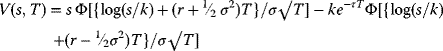
where
 , the probability that a normal distribution
N(0, 1) has values less than x, then one may calculate that V0 = V(s, T).
Consider the change of variable
and use it to establish the common form of the Black–Scholes formula, namely,
