5
Assets Allocation Using R
5.1 Risk Aversion and the Assets Allocation Process
The main objectives for asset allocation include the maximizing of returns, with/without periodic incomes derived from the returns. During these processes, the investor may freely use assets allocation to achieve such goals. Moreover, it certainly should not escape one's attention that the process of assets allocation is laden with the state of risk aversion on the part of the investors.
A growing body of research investigates whether investor risk aversion varies over time. Determining risk aversion is becoming increasingly important both in the United States and internationally for compliance and suitability purposes among financial advisors who are building portfolios for their clients. It appears that significant evidence has been established that risk aversion is time varying and that changes in risk aversion are primarily related to changes in investor expectations instead of historical market returns. Time-varying risk aversion carries important implications for the demand for risky assets if investors reduce demand for stocks when valuations are most attractive. It is noted that a statistically significant relation exists between time-varying risk aversion and net equity mutual fund flows, or a variable risk preference bias. It is found that net equity flows for more sophisticated investors, such as those who use index (versus active) mutual funds and purchase institutional equities.
Using a unique dataset with daily responses to a risk tolerance questionnaire from participants in a defined contribution plan, it is found that risk aversion is time-varying. It is also noted that investor expectations tend to be a better predictor of time-varying risk aversion than historical performance. So it appears that risk aversion is driven more by the unknown future than the known past! While investor expectations influence risk aversion over time, other investor attributes such as age, equity allocation, and salary appear to play an even greater role in shaping risk aversion. Time-varying risk aversion has important implications for the demand for risky assets since investors tend to shy away from risky assets when valuations are most attractive and when traditional portfolio theory would predict greater demand for equities to rebalance a portfolio. This effect is especially noteworthy given the increasing use of risk tolerance questionnaires (RTQs) by advisors when recommending an optimal client portfolio allocation. This is significant because the primary reason that individual investors underperform institutional investors is their tendency to sell equity mutual funds during a bear market!
Sophisticated investors, such as those who use index (versus active) mutual funds and buy institutional share classes (i.e., have more wealth and, therefore, more implied investing human capital), exhibit lower time-varying risk aversion. It is also noted that a consistent negative relation between time-varying risk aversion and net equity mutual fund flows may be established. Trail compensation, which provides the same incentive whether the client buys new funds to match their changing risk preferences, is associated with a lower variable risk preference bias.
5.2 Classical Assets Allocation Approaches
Asset allocation is the undertaking of an investment strategy in order to balance risk versus reward by adjusting the percentage of each asset in an investment portfolio according to the investor's risk tolerance, goals, and investment time frame.
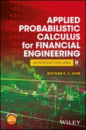
Figure 5.1 is a typical asset allocation pie chart.
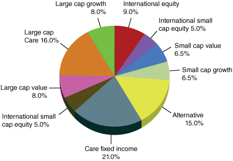
Figure 5.1 An asset investment pie chart – with a diverse portfolio.
It is not easy to measure the overall potential benefits from efficient financial planning: For a given portfolio, a specific investment decision may be analyzed in terms of two fundamental components, generally called alpha α and beta β:
- α is the luck/skill-based residual component associated with the various approaches of active financial management – such as security selection, tactical asset allocation, and so on
- β is the systematic risk exposures of the portfolio – normally achieved via asset allocation.
α and β are at the heart of traditional performance analysis. However, they are only two of many important financial planning decisions, such as savings and withdrawal strategies, which can have a substantial impact on the retirement outcome for an investor.
5.2.1 Going Beyond α and β
The notions of α and β (in particular α) have long challenged financial advisors and their clients:
- α allows a financial advisor to demonstrate (and potentially quantify) the excess returns generated, which can help justify fees.
- On the other hand, β (systematic risk exposures) helps to explain the risk factors of a portfolio to the market, that is, the asset allocation.
However, another concept gamma γ is designed to measure the value added achieved by an investor from making more sophisticated financial planning decisions. This value may be measured by calculating the certainty equivalent utility-adjusted retirement income across different scenarios. The Greek letter gamma, γ, is a widely used parameter in some areas of finance, such as in the trading of derivatives and in risk management.
5.2.2 γ Factors
The potential value, or gamma, γ, may be obtained from making five different “intelligent” financial planning decisions during retirement. A potential retiree has a number of risks, some of which are unique to retirement planning and are not serious concerns during accumulation. These five different factors are as follows:
- Asset Location and Withdrawal Sourcing: Tax-efficient investing for a retiree may be considered in terms of both “asset location” and intelligent withdrawal sequencing from accounts that differ in tax status. Asset location is defined as locating assets in the most tax-efficient account type. For example, it generally makes sense to place less tax-efficient assets (i.e., the majority of total return comes from dividends that are taxed as ordinary income), such as bonds, in retirement accounts (e.g., IRAs or 401(k)s) and more tax-efficient assets (i.e., the majority of total return comes from capital gains taxed at rates less than ordinary income), such as stocks, in taxable accounts. When thinking about withdrawal sequencing, it is prudent to withdraw monies from taxable accounts first and more tax-efficient accounts (e.g., IRAs or 401(k)s) later.
- Total Wealth Asset Allocation: Most techniques used for determining the asset allocation for a client are often relatively subjective and focus primarily on risk preference (i.e., an investor's aversion to risk) and ignore risk capacity (i.e., an investor's ability to assume risk). In practice, however, it is often believed that asset allocation should be based on a combination of risk preference and risk capacity, although primarily risk capacity. One determines an investor's risk capacity by evaluating the total wealth of the client, which is a combination of human capital (an investor's future potential savings) and financial capital. One may either use the market portfolio as the target aggregate asset allocation for each investor (as suggested by the Capital Asset Pricing Model) or build an investor-specific asset allocation that incorporates an investor's risk preferences. In both approaches, the financial assets are invested, subject to certain constraints, in order to achieve an optimal asset allocation that takes both human and financial capital into account.
- Annuity Allocation: Among retirees, one of the greatest fears is outliving one's savings! For example, a study by Allianz Life has shown that more retirees feared outliving their resources (61%) versus death (39%). Annuities allow a retiree to hedge against longevity risk and can, therefore, improve the overall efficiency of a retiree's portfolio. The contribution of an annuity within a total portfolio framework, (benefit, risk, and cost) should be considered before determining the appropriate amount and annuity type.
- Dynamic Withdrawal Strategy: Most retirement research has focused on static withdrawal strategies where the annual withdrawal during retirement is based on the initial account balance at retirement, increased annually for inflation. For example, a “5% withdrawal rate” would really mean a retiree may take a 5% withdrawal of the initial portfolio value and continue withdrawing that amount each year, adjusted for inflation. If the initial portfolio value was $2 million, and the withdrawal rate was 5%, the retiree would be expected to generate 5% of $2 million, or $100,000, in the first year. If inflation during the first year was 3%, the actual cash flow amount in the second year (in nominal terms) would be $103,000 (= $100,000 × 1.03). Using this approach the withdraw amount is based entirely on the initial income target, and is not updated based on market performance or expected investor longevity.
- Liability-Relative Optimization: Asset allocation methodologies commonly ignore the funding risks, like inflation and currency, associated with an investor's goals. By incorporating the liability into the portfolio optimization process it is possible to build portfolios that can better hedge the risks faced by a retiree. While these “liability-driven” portfolios may appear to be less efficient asset allocations when viewed from an asset-only perspective, one finds they are actually more efficient when it comes to achieving the sustainable retirement income.
On the other hand, each of these five gamma γ concepts may be thought of as actions and services provided by financial planners. One may take a practical function approach to quantify the benefit of different income-maximizing decisions. The goal of this approach is to provide some perspective, as well as quantify the potential benefits that can be realized by an investor (in particular a retiree) from using a gamma-optimized portfolio.
5.2.2.1 Measuring γ
One approach to measure the economic gain from making more intelligent financial planning decisions is to calculate the net present value of the additional income generated by the improved strategy, for example, to quantify the economic benefit that American investors can obtain from strategically timing the start of social security benefits (e.g., adjusting the initial claiming age). This approach does not require any explicit assumptions about subjective investor preferences.
5.2.2.2 How to Measure γ
For a single period, expected utility theory expects that an investor ranks alternative uncertain amounts of income by the expected utility of each. Letting I denote the random amount of income in the given period, then the expected utility of I is
where u(·) is an increasing concave utility function that reflects the risk tolerance of the investor.
Since values of u (·) are abstract undefined measures of “utility,” one may define the expected utility to the utility-adjusted certainty equivalent level of income:
which means that the investor is indifferent to the random amount of income I and the certain amount of income CE[I]. γ measures how much additional utility-adjusted income a strategy increases over and above the utility-adjusted income from a set of base-case decisions.
In the financial literature, several parametric forms of u(·) are commonly used. The most common one is the constant relative risk aversion (CRRA) utility function, which may be expressed as:
where θ is the risk tolerance parameter.
Owing to its analytical simplicity and its ability to represent a wide range of opinions toward risk with a single parameter, the CRRA utility function is used not only in single-period models, but also in multiperiod models.
Let It denote the random amount of income in period t, the expected utility of the sequence of incomes from periods 0 to T in these models is
where dt is the discount factor for period t. However, the parameter θ does have a role in the calculation of utility even if there is no uncertainty – because, in a multiperiod context, θ plays the following two roles:
- The investor's risk tolerance parameter
- The investor's elasticity of intertemporal substitution (EOIS) preference parameter.
It was pointed out by Epstein and Zin that there is no reason that the risk tolerance parameter and the EOIS parameter are equal. The reason for setting them equal is mathematical expediency. By recursively nesting the certainty equivalence function inside of the intertemporal utility function, Epstein and Zin formulated expected utility that makes these distinct parameters:
where
- Vt is the utility of the stream of income, starting at time t (measured in the same unit as income), and
- η is the investor's elasticity of intertemporal substitution preference parameter.
On the certainty equivalent operator, the t subscript denotes that it is conditional on what is known at time t.
The utility function generalizes the recursive expected utility maximization problem formulated by Lucas (1978), whereas gamma is derived from a measure of the utility of a given set of simulated income paths. Here, one may formulate a utility function with the same EOIS and risk parameters as the Epstein–Zin utility function that may be evaluated without recursion. This may be achieved by reversing the order of the nesting of intertemporal and risk components of utility. Thus, for each simulated income path, one may calculate its utility-equivalent constant income level based on the EOIS parameter, which is denoted as II. That is, for a given simulated income path, II is the constant amount of income with the same utility as the actual income path. This is given by

where
- It is the level of income in year t
- qt is the probability of surviving to at least year t
- r is the last year for which qt > 0
ρ is the investor's subjective discount rate (so that dt in (5.5) is qt(1 + ρ)−t Note that while (5.6) contains two preference parameters (ρ and η) that describe how the investor feels about having income to consume at different points in time, it does not show how the investor feels about risk. As was discussed already, one treats the elasticity of intertemporal substitution as a parameter distinct from the risk tolerance parameter. One may introduce the risk tolerance parameter next by treating the entire path as unknown and evaluating expected utility.
One may measure expected utility using the CRRA utility function with its risk tolerance parameter θ that we introduced in (5.3).
where
- M is the number of paths
- the subscript i denotes which of M paths is being referred to
pi is the probability of path i occurring which is set to 1/M.One may define Y as the constant value for II that yields this level of expected utility. This is the certainty equivalent of the stochastic utility-adjusted income II, and Y is given by
One may now define the gamma γ of a given strategy or a set of decisions as
As a base case, one may use the following parameter values:
Later, one may perform sensitivity analysis to explore the impact of how gamma γ is affected by the choice values for these parameter values.
5.2.3 The Mortality Model
Mortality may be modeled using the “Gompertz law of mortality”:
“The probability of a person dying increases at a relatively constant exponential rate as age increases.”
Here, one may use the formulation of Gompertz law for mortality – for which the Milevsky–Robinson form of this law is the probability of survival to age t ≤115 conditional on a life at age a, is given by
where
- m is the modal lifespan
- b is the dispersion coefficient.
One may use the Gompertz parameters that are fitted to the discrete, “Annuity 2000 Basic Table,” mortality table using the following procedure: the probability of having at least one member of a married couple surviving to age t is
Using this table, which contains the mortality rates per 1,000 persons (for males and females), ages 5–115, in Equation (5.12) – in which ![]() denotes the mortality rate for a person of the given age t and gender – one may compute the survival rates for persons of ages 65 to 115 for each gender, as follows:
denotes the mortality rate for a person of the given age t and gender – one may compute the survival rates for persons of ages 65 to 115 for each gender, as follows:
From this model, one may calculate the probability of a person, of a given gender, dying at age t > 65
For a given gender, the age which reaches its maximum value is the modal age for the given gender: m in (5.10). It has been shown that
| for male | m = 86 |
| for female | m = 90 |
For each gender, one may estimate the dispersion coefficient b in (5.10) by minimizing the sum of squared differences:
where qt is the survival probability given by the Gompertz model in (5.6). The SSD results are 10.48 for males and 8.63 for females.
For each gender, one may estimate the dispersion coefficient, b in (5.10), by minimizing the sum of squared differences, (5.14).
5.2.4 Sensitivity Analysis
To assess the impact of the asset allocation of the base case, one may recalculate Test 2 (say, bootstrapping by repeating each 10,000-trial Monte Carlo simulation 100 times) using different equity allocations.
One might note that for all equity allocations greater than the base case of 20%, the gamma estimate is almost within one standard error of the base case result. Hence, one may conclude that gamma varies little across base case asset allocations. To see the impact on gamma of varying the preference parameters for Test 2, one took the simulation from the initial bootstrap analysis that had the closest value to the average, which was 19.36%. Using this simulation, one varied the values of risk tolerance (θ), the subjective discount rate (ρ), and the elasticity of intertemporal substitution (η).
It has been found that varying θ had little impact on gamma.
5.2.4.1 The Elasticity of Intertemporal Substitution (EOIS)
To illustrate the role of the EOIS parameter, η, and its impact on gamma, consider a model in which a given amount of total wealth (financial assets plus human capital) is used to finance consumption over an infinite time horizon. Assume that the market offers a risk-free flat yield curve. If the single market interest rate equals the subjective discount factor (ρ), the optimal level of consumption is the same in every year regardless of the marginal rate of intertemporal substitution.
If the market interest rate is less than the subjective discount rate, the optimal consumption path is downward sloping:
- If the EOIS is high (η = 0.9), the optimal level of consumption starts high and the path is steeply sloped. However, if the EOIS is low (η = 0.1), the optimal consumption path is nearly flat.
This model of the sensitivity of gamma to the η parameter illustrates that gaging investors' willingness to reschedule income can be an important input to financial planning. While most financial planning questionnaires are designed to elicit information about an investor's investment horizon and risk tolerance, few seek to assess an investor's elasticity of intertemporal substitution.
5.3 Allocation with Time Varying Risk Aversion
5.3.1 Risk Aversion
In financial engineering, risk aversion is the behavior of humans (especially investors), when exposed to uncertainty, to try to reduce that uncertainty. For example, it is the reluctance of the investor to accept a bargain with an uncertain payoff rather than another bargain with a more certain, but possibly/usually lower, expected payoff. For example, a risk-averse investor may prefer to put the investment into a savings bank account with a low but guaranteed interest rate, rather than into a stock that may have much higher expected returns, but also involves a chance of losing value.
Such psychological characteristics are illustrated in Figure 5.2.

Figure 5.2 Utility function of a risk-seeking individual. Risk aversion (red) contrasted to risk neutrality (yellow) and risk loving (orange) in different settings.(a) A risk averse utility function is concave from below, while a risk loving utility function is convex from below.(b) In standard deviation-expected value space, risk averse indifference curves are upward sloped.(c) With fixed probabilities of two alternative states 1 and 2, risk averse indifference curves over pairs of state-contingent outcomes are convex.
5.3.1.1 Example of a Risk-Averse/Neutral/Loving Investor
Suppose an investor is given the choice between the following two scenarios:
- One with a guaranteed payoff
- One without
In the guaranteed scenario (1), the investor receives $100,000 zillion.
In the uncertain scenario (2), a coin is flipped to decide whether the person receives $200,000 (that is, 2 × $100,000) or nothing. The expected payoff for both scenarios is $100,000, meaning that an individual who was insensitive to risk would not care whether they took the guaranteed payment or the gamble.
However, individuals may have different risk attitudes.
An investor is said to be the following:
- Risk-averse (or risk-avoiding): If the investor would accept a certain payment (certainty equivalent) of less than $100,000 (e.g., $80,000), rather than taking the gamble and possibly receiving nothing.
- Risk-neutral: If the investor is indifferent between the bet and a certain $100,000 payment.
- Risk-seeking: If the investor would accept the bet even when the guaranteed payment is more than $100,000 (e.g., $120,000).
The average payoff of the gamble, called its expected value, is $100,000. The dollar amount that the individual would accept instead of the bet is called the certainty equivalent, and the difference between the expected value and the certainty equivalent is called the risk premium, that is,
For risk-averse individuals, the risk premium is positive, for risk-neutral persons it is zero, and for risk-loving individuals their risk premium becomes negative.
5.3.1.2 Expected Utility Theory
In expected utility theory, a person (including an investor) has a utility function u(x), where x represents the value that he might receive in money or goods (in the above example x could be 0 or 100).
Time does not come into this consideration, so inflation does not appear. (The utility function u(x) is defined only up to positive linear affine transformation – in other words, a constant offset could be adjusted (added) to the value of u(x) for all x, and/or u(x) could be multiplied by a positive constant factor, without affecting the conclusions).
An agent possesses risk aversion if and only if the utility function is concave. For instance u(0) could be 0, u(100) might be 10, u(60) might be 7, and for comparison u(50) might be 6.
The expected utility of the above bet (with a 50% chance of receiving 100 and a 50% chance of receiving 0) is
and if the person has the utility function with u(0) = 0, u(50) = 6, and u(100) = 10, then the expected utility of the bet equals 5, which is the same as the known utility of the amount 40. Hence, the certainty equivalent is 40.
The risk premium is ($50 − $40) = $10, or in proportional terms
or 25%, where $50 is the expected value of the risky bet
This risk premium means that the investor would be willing to sacrifice as much as $10 in expected value in order to achieve perfect certainty about how much money will be received. That is, the person would be indifferent between the bet and a guarantee of $40, and would prefer anything over $40 to the bet.
For a more wealthy investor, the risk of losing $100 would be less significant, and for such small amounts his utility function would be likely to be almost linear, for instance if u(0) = 0 and u(100) = 10, then u(40) might be 4.0001 and u(50) might be 5.0001.
5.3.1.3 Utility Functions
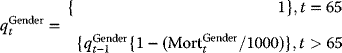
The utility function for perceived gains has two key properties: an upward slope and concavity.
- The upward slope implies that the investor feels that more is better: A larger amount received yields greater utility, and for risky bets the person would prefer a bet which is first-order stochastically dominant over an alternative bet (i.e., if the probability mass of the second bet is pushed to the right to form the first bet, then the first bet is preferred).
- The concavity of the utility function implies that the investor is risk averse: A sure amount would always be preferred over a risky bet having the same expected value; moreover, for risky bets the investor would prefer a bet that is a mean-preserving contraction of an alternative bet (that is, if some of the probability mass of the first bet is spread out without altering the mean to form the second bet, then the first bet is preferred) (Figures 5.3a, b, and c).
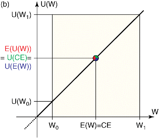
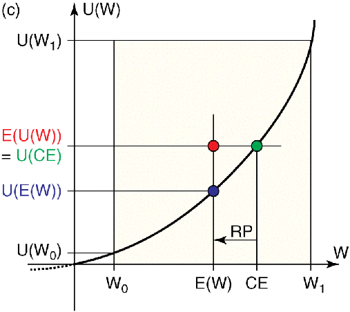
Figure 5.3 (a) Utility function of a risk-averse (risk-avoiding) investor. (b) Utility function of a risk-neutral investor. (c) Utility function of a risk-seeking individual. CE: certainty equivalent, E(U(W)): expected value of the utility (expected utility) of the uncertain payment, E(W): expected value of the uncertain payment, U(CE): utility of the certainty equivalent, U(E(W)): utility of the expected value of the uncertain payment, U(W0): utility of the minimal payment, U(W1): utility of the maximal payment, W0: minimal payment, W1: maximal payment, RP: risk premium.
A person is given the choice between two scenarios, one with a guaranteed payoff and one without. In the guaranteed scenario, the person receives $50. In the uncertain scenario, a coin is flipped to decide whether the person receives $100 or nothing. The expected payoff for both scenarios is $50, meaning that an individual who was insensitive to risk would not care whether they took the guaranteed payment or the gamble. However, individuals may have different risk attitudes.
5.3.2 Utility of Money
In expected utility theory, an investor has a utility function u(x), where x represents the value that an investor might receive in money or goods (in the above example x could be 0 or 100).
Time does not come into this calculation, so inflation does not appear. (The utility function u(x) is defined only up to positive linear affine transformation – namely, a constant offset could be added to the value of u(x) for all x, and/or u(x) could be multiplied by a positive constant factor, without affecting the conclusions).
An agent possesses risk aversion if and only if the utility function is concave. For instance u(0) could be 0, u(100) might be 20, u(40) might be 10, and for comparison u(50) might be 12.
The expected utility of the above bet (with a 50–50 chance of receiving 0 and a 50–50 chance of receiving 100) is
and if the person has the utility function with u(0) = 0, u(40) = 10, and u(100) = 20, then the expected utility of the bet equals
which is the same as the known utility of the amount 40: u(40) = 10.
Hence the certainty equivalent is 40.
The risk premium is ($50 − $40) = $10, or in proportional terms
or 25%, where $50 is the expected value of the risky bet
This risk premium means that the investor would be willing to sacrifice as much as $10 in expected value in order to achieve perfect certainty about how much money will be received. That is, the person would be indifferent between the bet and a guarantee of $40, and would prefer anything over $40 to the bet.
5.4 Variable Risk Preference Bias
It appears that there is a growing body of evidence of time-varying risk aversion.
Using a unique data set with daily responses to a risk tolerance questionnaire from participants in a defined contribution plan, one finds significant evidence that
- risk aversion is time-varying, and that
- changes in risk aversion are primarily related to changes in investor expectations instead of historical market returns.
Time-varying risk aversion has important implications for the demand for risky assets if investors reduce demand for stocks when valuations are most attractive.
- One may note a statistically significant relation between time-varying risk aversion and net equity mutual fund flows, or a variable risk preference bias.
- One may also find that net equity flows for more sophisticated investors, such as those who use index (versus active) mutual funds and purchase institutional share classes, exhibit lower time-varying risk aversion.
- One may also find a statistically significant negative relation between time-varying risk aversion and net equity mutual fund flows.
Hence, financial investment advisor compensation models focused on trail commissions may provide a valuable debiasing incentive that makes investors less susceptible to the variable risk preference bias.
5.4.1 Time-Varying Risk Aversion
Recent research in financial engineering provides significant evidences. S&P 500 index levels, from January 2000 through September 2010, showed the following:
- The average investor risk aversion is not constant over time.
- The maximum average monthly risk aversion score over the data series was 5.405, while the minimum average score was 4.525.
- The overall monthly average risk aversion score was 4.949.
- These changes represent a significant magnitude of variation because the potential scores are bounded by 3.000 and 9.000, where a score of 3.000 indicates a low level of risk aversion and a score of 9.000 indicates a high level of risk aversion.
5.4.1.1 The Rationale Behind Time-Varying Risk Aversion
While the average investor risk tolerance changes over time, there are a number of other investor and market characteristics that affect risk aversion. Two potential reasons of risk aversion are
- historical experiences (i.e., past returns) and
- future expectations of stock market performance.
The research has shown that there is a significant relation between risk aversion score decile and net equity mutual fund flows, CAPE Ratio, and future one-year returns. The negative relation between risk aversion and net equity flows suggests the following:
- Investors tend to favor equities when risk aversion is the lowest, which is also when markets have the least attractive valuations based on the CAPE Ratio and lowest future one-year returns.
- Investors appear to be less attracted to stock funds when valuations are most.
5.4.1.2 Risk Tolerance for Time-Varying Risk Aversion
Since risk aversion is time-varying, it is possible that the “run-of-the-mill” risk tolerance questionnaires (RTQs) may contribute to individual investor underperformance if the scores influence asset allocation selected by the plan providers. The more sophisticated investors may be less susceptible to risk preference bias.
One way to determine the relative investor sophistication is to look at the historical relation between net equity mutual fund flows for different types of mutual funds and risk aversion over time. The seasoned investor with constant risk preferences would rationally rebalance to equity mutual funds during a bear market. A biased investor may be less attracted to equity funds as valuations fall, increasing the portfolio share of safe assets when valuations of risky assets are most attractive. One may use three different methods to classify investors based on net equity mutual fund flows:
- Sort by whether funds are actively or passively managed. Passive mutual funds are assumed to be those classified as “index” funds by Morningstar, Inc., while all other mutual funds are considered actively managed funds. There is evidence that investors in passive funds are more sophisticated than investors in active funds that are most often sold through the broker channel.
- Classify mutual funds into four different fund groups: broker-sold, institutional, investor, or retirement.
- One may further decompose the broker-sold category by the form of compensation paid to the financial advisor. Differences in the method of compensation provided through share class structure may influence whether the advisor gains from debiasing a client who is tempted to shift the portfolio to safety during an equity market decline.
5.5 A Unified Approach for Time Varying Risk Aversion
Although traditional finance theory assumes that risk aversion is not time-varying, there is a growing body of empirical research that suggests that risk preferences change with market conditions. Using a unique dataset with daily responses to a risk tolerance questionnaire from participants in a defined contribution plan, one may find significant evidence that risk aversion is time-varying. It is also noted that investor expectations tend to be a better predictor of time-varying risk aversion than historical performance. Thus, it seems that risk aversion is driven more by the unknown future than the known past.
While investor expectations influence risk aversion over time, other investor attributes (such as age, equity allocation, and salary, etc.) appear to play an even greater role in shaping risk aversion. Time-varying risk aversion has important implications for the demand for risky assets since investors tend to avoid risky assets when valuations are most attractive and when traditional portfolio theory would predict greater demand for equities to rebalance a portfolio. This effect is especially noteworthy given the increasing use of the “traditional” RTQs by investment advisors when recommending an optimal client portfolio allocation. This is important because the primary reason that individual investors underperform institutional investors is their tendency to sell equity mutual funds during a bear market.
More sophisticated investors, such as those who use index (versus active) mutual funds and buy institutional share classes, exhibit lower time-varying risk aversion. It is also noted that a consistent negative relation between time-varying risk aversion and net equity mutual fund flows when sorted by fees. Trail compensation, which provides the same incentive whether the client buys new funds to match their changing risk preferences, is associated with a lower variable risk preference bias. Financial advisor compensation schemes that provide greater compensation for acceding to variable risk preference biases are associated with a failure to debias. This finding is consistent with research on perverse incentives from traditional commission.
5.6 Assets Allocation Worked Examples
5.6.1 Worked Example 1: Assets Allocation Using R
The Black–Litterman (B–L) Asset Allocation Model
Overview
Combining information from two sources to create an estimate of expected returns:
- Source 1: What does the current market tell us about the expected excess returns? Implied excess equilibrium returns?
- Source 2: What views does the investment manager have about particular stocks, sectors, asset classes, or country?
The B–L model combines these different sources to produce estimates of excess returns.
Combining predicted and implied returns
Basic Notation
- τ = A scalar (assume τ = 1).
- S = Variance–Covariance matrix for all assets under consideration
- Ω = Uncertainty surrounding your views.
- Π = Implied excess returns
- Q = Views on expected excess returns for some or all assets
- P = Link matrix identifying which assets you have views about
Understanding the Formula Splitting into two sections for better understanding
Consider the second section first:

We are combining implied excess returns with our own views on excess returns: A weighted average
What are the weights?
The investor about his/her views relative to the implied excess returns.
-How confident?
Ω will be large ⇒ Ω−1 will be small
Understanding the formula:
The first part of this formula:
- τ implies excess returns and our views add up to 1.
- Namely, the formula is just a weighted average!
Consider a worked example:
Consider 1 stock: AMZN (Amazon.com)
- The implied excess returns are 0.74% per month and the variance is 2.018%
- We predict excess returns of 2% per month. The uncertainty surrounding this view is reflected by a variance of 0.50%

- Assume τ = 1, P = 1
Substituting into the B–L formula:
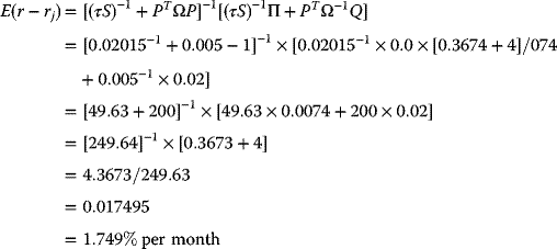
Does this estimate make sense?
Since we are confident about our views, now, try a more complicated example:
Incorporating Investor Views:
- Analysts tell you that AEP has found a way to store electricity. Based on this breakthrough, they expect AEP to outperform XOM by 1% per month.
- Given the current economic conditions, we think that INTC will outperform AMZN by 1.75% per month.
- Relative views are common in reality.
- Absolute views, such as AEP having returns of 2% per month, are much less common.
Views versus Implied Excess Returns:
- View (1): AEP outperforms XOM by 1% per month
- The difference in implied excess returns is −0.32% per month.
- One would expect that incorporating these views would lead to an increase in one's holdings of AEP and a decrease in XOM:0.0092.
- View (2): INTC will outperform AMZN by 1.75% per month.
- The difference in implied excess returns is 0.18% per month.
- We would expect that incorporating our view would increase our holdings of INTC and reduce our holdings of AMZN.
The views expressed above are relative views of assets.
Incorporating Our Views:
To link our views to implied excess returns, we need a link matrix, P.
Matrix P is constructed in the following way:
Each row represents a view, each column represents a company
| INTC | AEP | AMZN | MRK | XOM | |||
| View 1 | [ | 0 | 1 | 0 | 0 | −1 | ] |
| P = | [ | ] | |||||
| View 2 | [ | 1 | 0 | −1 | 0 | 0 | ] |
| [ | ] | ||||||
| View 3 | [ | 0.5 | 0 | 0.5 | −0.5 | −0.5 | ] |
The View Vector and Uncertainty
What do Q and Ω look like?
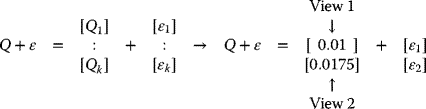
where

Calculating Ω
There is no best way to calculate Ω. It will depend on how confident you are of your predictions.
Black and Litterman recommend
We have assumed that τ = 1, and so we can ignore it!
The well-known classical Black–Litterman models for asset allocation may be represented by the following two schematic illustrations:
Figures 5.4a and 5.5a.

Figure 5.4a Classical Black–Litterman model I.

Figure 5.4b StockPortfolio-1.
5.6.2 Worked Example 2: Assets Allocation Using R, from CRAN
Harry Markowitz on Assets Allocation: R package PortfolioAnalytics
In the R domain
> install.packages("PortfolioAnalytics")> library(PortfolioAnalytics)> ls("package:PortfolioAnalytics")[1] "ac.ranking" "add.constraint"[3] "add.objective" "add.objective_v1"[5] "add.objective_v2" "add.sub.portfolio">> install.packages("stockPortfolio ")Installing package into ‘C:/Users/Bert/Documents/R/win-library/3.2'(as 'lib' is unspecified)--- Please select a CRAN mirror for use in this session ---
A CRAN mirror is selected.
>trying URL'https://stat.ethz.ch/CRAN/bin/windows/contrib/3.2/stockPortfolio_1.2.zip'Content type 'application/zip' length 115410 bytes (112 KB)downloaded 112 KBpackage 'stockPortfolio' successfully unpacked and MD5 sumscheckedThe downloaded binary packages are inC:UsersBertAppDataLocalTempRtmpeEU8Podownloaded_packages> library(stockPortfolio)> ls("package:stockPortfolio")[1] "adjustBeta" "getCorr" "getReturns" "optimalPort"[5] "portCloud" "portPossCurve" "portReturn" "stockModel"[9] "testPort"
>> #1 stockPortfolio-package> # Build and manage stock models and portfolios>> ===> two examples of downloading data <===> ## Not run: grEx1 <- getReturns(c('C','BAC'), start='2004-01-01', end='2008-12-31')> ## Not run: grEx2 <- getReturns(c('KEY', 'WFC', 'JPM', 'AMR','BIIB', 'AMGN'))> ===> build four models <===#> data(stock99)> data(stock94Info)> non <- stockModel(stock99, drop=25, model='none',+ industry=stock94Info$industry)> sim <- stockModel(stock99, model='SIM',+ industry=stock94Info$industry, index=25)> ccm <- stockModel(stock99, drop=25, model='CCM',+ industry=stock94Info$industry)> mgm <- stockModel(stock99, drop=25, model='MGM',+ industry=stock94Info$industry)> ===> build optimal portfolios <===#> opNon <- optimalPort(non)> opSim <- optimalPort(sim)> opCcm <- optimalPort(ccm)> opMgm <- optimalPort(mgm)> ===> test portfolios on 2004-9 <===#> data(stock04)> tpNon <- testPort(stock04, opNon)Warning message:In testPort(stock04, opNon) : Allocation X was standardized> tpSim <- testPort(stock04, opSim)Warning message:In testPort(stock04, opSim) : Allocation X was standardized> tpCcm <- testPort(stock04, opCcm)Warning message:In testPort(stock04, opCcm) : Allocation X was standardized> tpMgm <- testPort(stock04, opMgm)Warning message:In testPort(stock04, opMgm) : Allocation X was standardized>> ===> compare performances <===#> plot(tpNon)> # Figure 5.4b StockPortfolio-1
>> lines(tpSim, col=2, lty=2)> # Figure 5.5b StockPortfolio-2>> lines(tpCcm, col=3, lty=3)> # Figure 5.6 StockPortfolio-3>> lines(tpMgm, col=4, lty=4)
> # Figure 5.7 StockPortfolio-4>> legend('topleft', col=1:4, lty=1:4, legend=c('none', 'SIM',+ 'CCM', 'MGM'))> # Figure 5.8 StockPortfolio-5

Figure 5.5a Classical Black–Litterman model II.
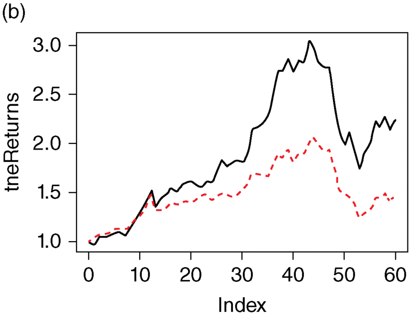
Figure 5.5b StockPortfolio-2.

Figure 5.6 StockPortfolio-3.
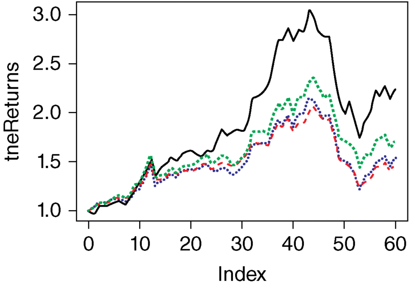
Figure 5.7 StockPortfolio-4.

Figure 5.8 StockPortfolio-5. SIM (Grupo Simec SAB de CV) – Computing and Technology, CCM – Medical Services, and MGM – MGM Resorts International.
5.6.3 Worked Example 3: The Black–Litterman Asset
Review Questions and Exercises
- At the heart of traditional performance analysis are two factors α and β.
Briefly describe these two factors, giving some common examples.
-
- Describe and contrast investors who are
- risk-averse
- risk-neutral, and
- risk-loving
- Suggest some useful approaches suitable for each one of these three types of investors.
- Describe and contrast investors who are
- Literature Survey:
A considerable amount of literature has been developed in the areas supporting the analytical approaches to assets allocation. Much of these materials are readily available in the Internet sources. A typical example is the following paper by Robert Merton (1973) available at conpapers.repec.org/article/ecmemetrp/default38.htm
- Study this online paper and
- Comment on the following issues:
“We use the structure imposed by Merton's (1973) ICAPM to obtain monthly estimates of the market-level risk-return relationship from the cross-section of equity returns. Our econometric approach sidesteps the specification of time-series models for the conditional risk premium and volatility of the market portfolio. We show that the risk-return relation is mostly positive but varies considerably over time. It co-varies positively with counter-cyclical state variables. The relationship between the risk premium and hedge-related risk also exhibits strong time-variation, which supports the empirical evidence that aggregate risk aversion varies over time. Finally, the ICAPM's two components of the risk premium show distinctly different cyclical properties. The volatility component exhibits a counter-cyclical pattern whereas the hedging component is less related to the business cycle and falls below zero for extended periods. This suggests the market serves an important hedging role for long-term investors.”
These issues are found in a paper by
Brandt, M. W. and Wang, L. P. (2010) Measuring the time-varying risk-return relation from the cross-section of equity returns.
- Do you agree, or disagree with the conclusions in this paper? And why?
- An exercise in financial modeling for assets allocation.
The GARCH Process and the CRAN Package tseries
The generalized autoregressive conditional heteroskedasticity process
The generalized autoregressive conditional heteroskedasticity (GARCH) process is an econometric term developed in 1982 by Robert F. Engle, an economist and the 2003 winner of the Nobel Memorial Prize for Economics, to describe an approach to estimate volatility in financial markets. There are several forms of GARCH modeling. The GARCH process is often preferred by financial modeling professionals because it provides a more real-world context than other forms when trying to predict the prices and rates of financial instruments.
The general process for a GARCH model involves three steps:
- The first is to estimate a best-fitting autoregressive model.
- The second is to compute autocorrelations of the error term.
- The third is to test for significance.
GARCH models are used by financial professionals in several areas, including trading, investing, hedging, and dealing. Two other widely used approaches to estimate and predict financial volatility are as follows:
- The classic historical volatility (VolSD) method
- The exponentially weighted moving average volatility (VolEWMA) method.
The GARCH Process
GARCH models help to describe financial markets in which volatility can change, becoming more volatile during periods of financial crises or world events and less volatile during periods of relatively calm and steady economic growth. On a plot of returns, for example, stock returns may look relatively uniform for the years leading up to a financial crisis such as the one in 2007. In the time period following the onset of a crisis, however, returns may swing wildly from negative to positive territory. Moreover, the increased volatility may be predictive of volatility going forward. Volatility may then return to levels resembling that of precrisis levels or be more uniform going forward. A simple regression model does not account for this variation in volatility exhibited in financial markets and is not representative of the "black swan" events that occur more than one would predict.
GARCH Models for Asset Returns
GARCH processes differ from homoskedastic models, which assume constant volatility and are used in basic ordinary least squares (OLS) analysis. OLS aims to minimize the deviations between data points and a regression line to fit those points. With asset returns, volatility seems to vary during certain periods of time and depends on past variance, making a homoskedastic model not optimal or suitable.
GARCH processes, being autoregressive, depend on past squared observations and past variances to model for current variance. They are widely used in finance owing to their effectiveness in modeling asset returns and inflation. A GARCH process aims to minimize errors in forecasting by accounting for errors in prior forecasting, enhancing the accuracy of ongoing predictions.
More on the GARCH Process: http://www.investopedia.com/terms/g/generalalizedautogregressiveconditionalheteroskedasticity.asp#ixzz4XwGOV3MI
And now consider a CRAN package based on GARCH:
Computational Finance
| Description | Time series analysis and computational finance. |
| Depends | R (>= 2.10.0) |
| Imports | graphics, stats, utils, quadprog, zoo |
| License | GPL-2 |
| NeedsCompilation | yes |
| Author | Adrian Trapletti [aut], |
| Kurt Hornik [aut, cre], | |
| Blake LeBaron [ctb] (BDS test code) | |
| Maintainer | Kurt Hornik <[email protected]> |
| Repository | CRAN |
| Date/Publication | 2017-01-17 12:33:40 |
| Description | Download historical financial data from a given data provider over the WWW. |
Usage
get.hist.quote(instrument = "^gdax", start, end,quote = c("Open", "High", "Low", "Close"),provider = c("yahoo", "oanda"),method = NULL,origin = "1899-12-30",compression = "d",retclass = c("zoo", "ts"),quiet = FALSE,drop = FALSE)
Arguments
| instrument | a character string giving the name of the quote symbol to download. See the webpage of the data provider for information about the available quote symbols. |
| start | an R object specifying the date of the start of the period to download. This must be in a form which is recognized by as.POSIXct, which includes R POSIX date/time objects, objects of class "date" (from package date) and "chron" and "dates" (from package chron), and character strings representing dates in ISO 8601 format. Defaults to 1992-01-02. |
| end | an R object specifying the end of the download period, see above. Defaults to yesterday. |
| quote | a character string or vector indicating whether to download opening, high, low, or closing quotes, or volume. For the default provider, this may be specified as "Open", "High", "Low", "Close", "AdjClose", and "Volume", respectively. For the provider "oanda", this argument is ignored. Abbreviations are allowed. |
| provider | a character string with the name of the data provider. Currently, "yahoo" and "oanda" are implemented. See http://quote.yahoo.com/and https://www.oanda.com/for more information. |
| method | tool to be used for downloading the data. See download.file for the available download methods and the default settings. |
| origin | an R object specifying the origin of the Julian dates, see above. Defaults to 1899-12-30 (Popular spreadsheet programs internally also use Julian dates with this origin). |
| compression | Governs the granularity of the retrieved data; "d" for daily, "w" for weekly or "m" for monthly. Defaults to "d". For the provider "oanda", this argument is ignored. |
| retclass | character specifying which class the return value should have: can be either "zoo" (with "Date" index), or "ts" (with numeric index corresponding to days since origin). |
| quiet | logical. Should status messages (if any) be suppressed? |
| Drop | logical. If TRUE the result is coerced to the lowest possible dimension. Default is FALSE. |
Value
A time series containing the data either as a "zoo" series (default) or as a "ts" series. The "zoo" series is created with zoo and has an index of class "Date". If a "ts" series is returned, the index is in physical time, that is, weekends, holidays, and missing days are filled with NAs if not available. The time scale is given in Julian dates (days since the origin).
Author(s)
A. Trapletti
See Also
zoo, ts, as.Date, as.POSIXct, download.file;http://quote.yahoo.com/, https://www.oanda.com/
- Portfolio optimization using the CRAN packages: PortfolioAnalytics and DEoptim
Here, one may consider two CRAN packages for portfolio optimization:
- PortfolioAnalytics enables one to obtain a numerical portfolio solution for a numerical solution for some given objectives and/or objective functions.
- DEoptim is then evoked to provide the numerical optimization.
These two CRAN packages are separately described, each followed by an illustrative worked example.
(1) Package “PortfolioAnalytics” April 19, 2015
| Type | Package |
| Title | Portfolio analysis, including numerical methods for optimization of portfolios |
| Version | 1.0.3636 |
| Date | 2015-04-18 |
| Maintainer | Brian G. Peterson <[email protected]> |
| Description | Portfolio optimization and analysis routines and graphics. |
| Depends | R (>= 2.14.0), zoo, xts (>= 0.8), foreach, PerformanceAnalytics (>= 1.1.0) |
| Suggests | quantmod, DEoptim(>= 2.2.1), iterators, fGarch, Rglpk, quadprog, ROI (>= 0.1.0), ROI.plugin.glpk (>= 0.0.2), ROI.plugin.quadprog (>= 0.0.2), ROI.plugin.symphony (>= 0.0.2), pso, GenSA, corpcor, testthat, nloptr (>= 1.0.0), MASS, robustbase |
| License | GPL |
| Copyright (c) | 2004-2015 |
| NeedsCompilation | yes |
| Authors | Brian G. Peterson [cre, aut, cph], Peter Carl [aut, cph], Kris Boudt [ctb, cph], Ross Bennett [ctb, cph], Hezky Varon [ctb], Guy Yollin [ctb], R. Douglas Martin [ctb] |
| Repository | CRAN |
| Date/Publication | 2015-04-19 07:38:57 |