
Chapter 4 explored collaborative filtering and using the KNN method. A few more important methods are covered in this chapter: matrix factorization (MF), singular value decomposition (SVD), and co-clustering. These methods (along with KNN) fall into the model-based collaborative filtering approach. The basic arithmetic method of calculating cosine similarity to find similar users falls into the memory-based approach. Each approach has pros and cons; depending on the use case, you must select the suitable approach.
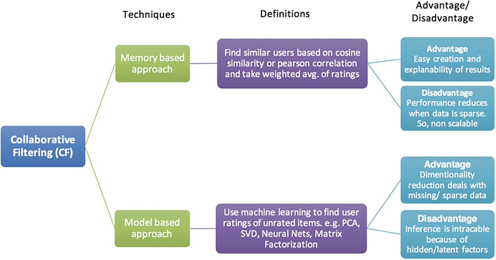
A framework exposes the classification of collaborative filtering. It classifies into 2 techniques: memory-based approach and model-based approach. The definitions, advantages, and disadvantages are exposed.
The two approaches of collaborative filtering explained
The memory-based approach is much easier to implement and explain, but its performance is often affected due to sparse data. But on the other hand, model-based approaches, like MF, handle the sparse data well, but it’s usually not intuitive or easy to explain and can be much more complex to implement. But the model-based approach performs better with large datasets and hence is quite scalable.
This chapter focuses on a few popular model-based approaches, such as implementing matrix factorization using the same data from Chapter 4, SVD, and co-clustering models.
Implementation
Matrix Factorization, Co-Clustering, and SVD
The following implementation is a continuation of Chapter 4 and uses the same dataset.
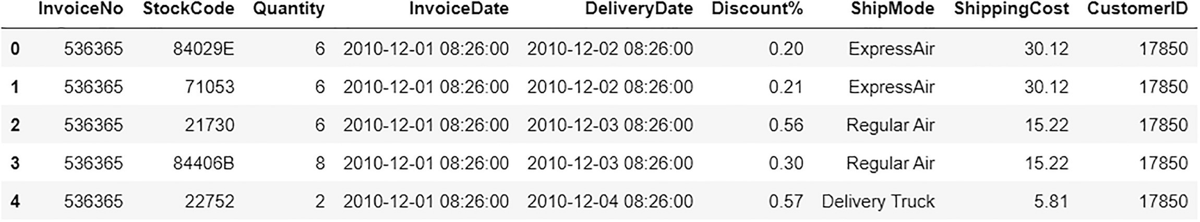
A data frame exposes the input data that include invoice number, stock code, quantity, invoice date, delivery date, discount percentage, ship mode, shipping cost, and customer I D.
Input data
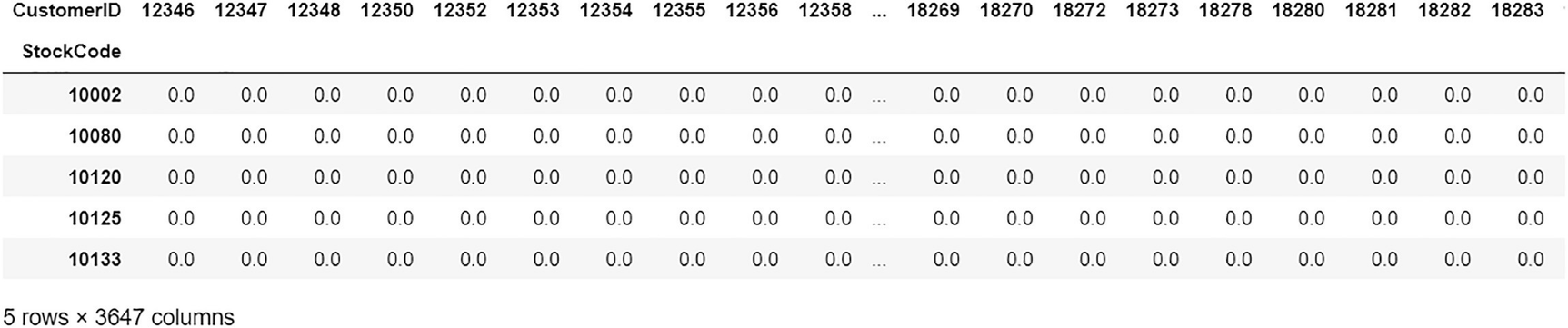
A data frame exposes the data of items purchased. The customer I D and stock code are represented.
Item purchase DataFrame/matrix
This chapter uses the Python package called surprise for modeling purposes. It has implementations of popular methods in collaborative filtering, like matrix factorization, SVD, co-clustering, and even KNN.
First, let’s format the data into the proper format required by the surprise package.
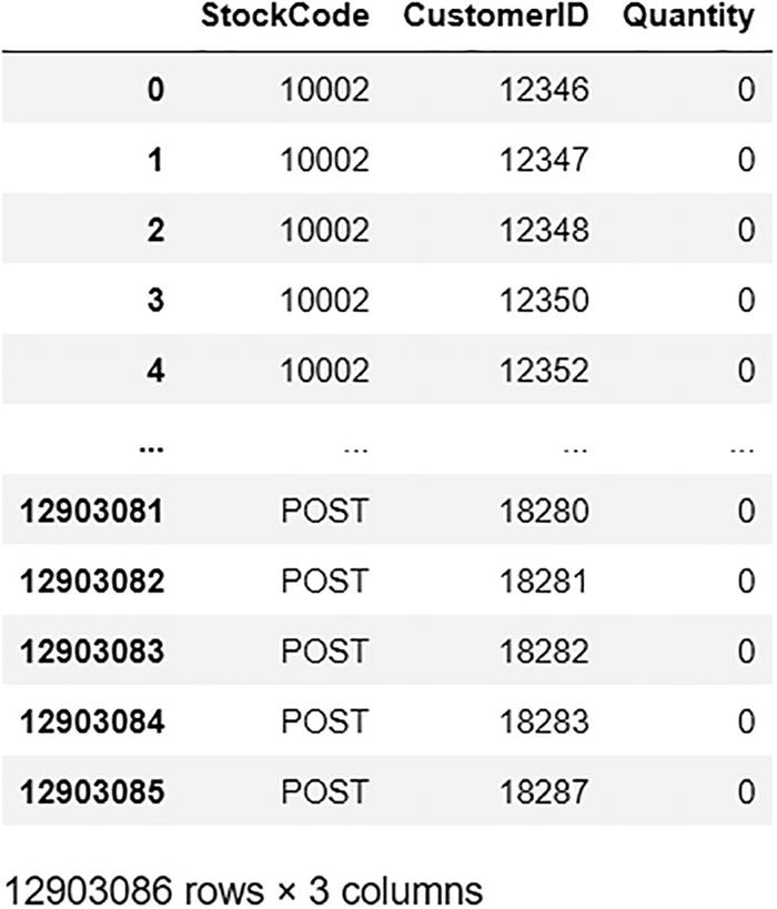
A data frame exposes the output of stacked item purchases. The stock code, customer I D, and quantity are represented. Every quantity is observed with 0.
Stacked item purchase DataFrame/matrix
As you can see, items_purchase_df has 3538 unique items (rows) and 3647 unique users (columns). The stacked DataFrame is 3538 × 3647 = 12,903,086 rows, which is too big to pass into any algorithm.
Let’s shortlist some customers and items based on the number of orders.
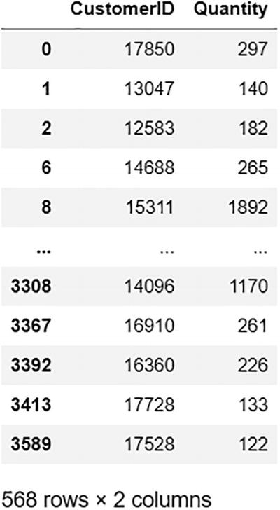
A data frame exposes the count of the customer. The customer I D and the quantity are represented. The model of the data frame: 568 rows and 2 columns.
Customer count DataFrame
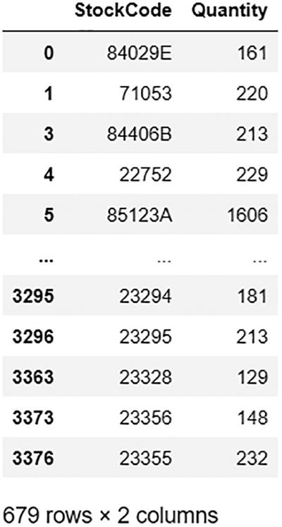
A data frame exposes the output of item count. The customer I D and the quantity are represented. The model of the data frame: 679 rows and 2 columns.
Item count DataFrame
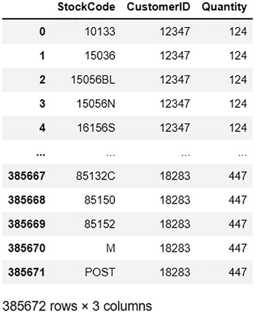
A data frame exposes the output of shortlisted data. The stock code, customer I D, and quantity are represented. The data frame model: 385672 rows and 3 columns.
The final shortlisted DataFrame
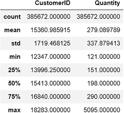
A data frame reports the shortlisted data. The customer I D, and quantity along with the mean, count, minimum, and maximum values are exposed.
Describes the shortlisted DataFrame
You can see from the output that the count has significantly reduced to 385,672 records, from 12,903,086. But this DataFrame is to be formatted further using built-in functions from the surprise package to be supported.
The range has been set as 0,5095 because the maximum quantity value is 5095.
The final formatted data is ready.
Implementing NMF
Let’s start by modeling the non-negative matrix factorization method.
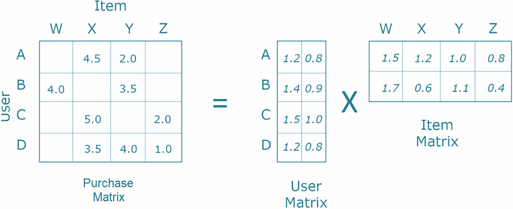
A representation of matrix factorization. The purchase matrix is equal to the user matrix multiplied by the item matrix. A, B, C, and D indicate the users. W, X, Y, and Z indicate the items.
Matrix factorization
The RMSE and MAE are moderately high for this model, so let’s try the other two and compare them at the end.
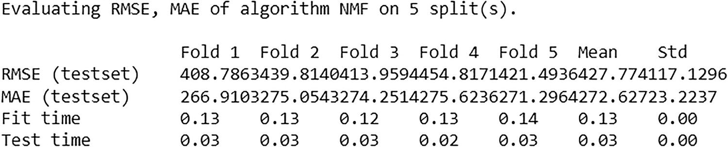
A representation exhibits the outcome of cross-validation for N M F. Evaluating R M S E, M A E, of algorithm N M F on 5 splits is exposed.
Cross-validation output for NMF
The cross-validation shows that the average RMSE is 427.774, and MAE is approximately 272.627, which is moderately high.
Implementing Co-Clustering
Co-clustering (also known as bi-clustering) is commonly used in collaborative filtering. It is a data-mining technique that simultaneously clusters the columns and rows of a DataFrame/matrix. It differs from normal clustering, where each object is checked for similarity with other objects based on a single entity/type of comparison. As in co-clustering, you check for co-grouping of two different entities/types of comparison for each object simultaneously as a pairwise interaction.
The RMSE and MAE are very low for this model. Until now, this has performed the best (better than NMF).
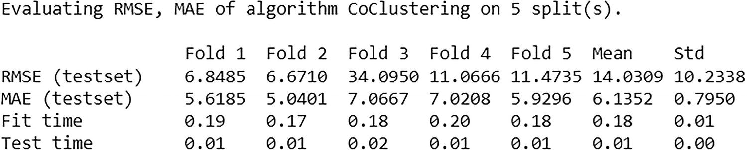
A representation exposes the output of cross-validation for co-clustering. Evaluating R M S E and M A E of algorithm co-clustering on 5 splits are depicted.
Cross-validation output for co-clustering
The cross-validation shows that the average RMSE is 14.031, and MAE is approximately 6.135, which is quite low.
Implementing SVD
Singular value decomposition is a linear algebra concept generally used as a dimensionality reduction method. It is also a type of matrix factorization. It works similarly in collaborative filtering, where a matrix with rows and columns as users and items is reduced further into latent feature matrixes. An error equation is minimized to get to the prediction.
The RMSE and MAE are significantly high for this model. Until now, this has performed the worst (worse than NMF and co-clustering).
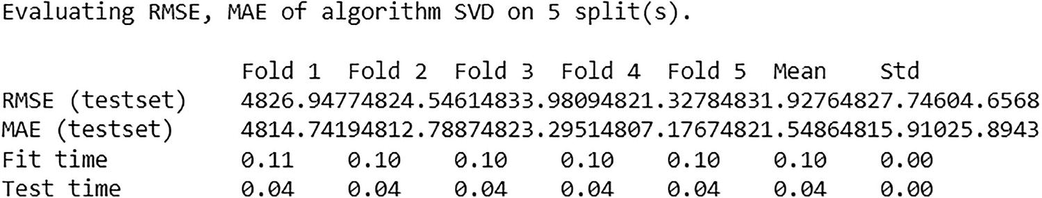
A representation exposes the output of cross-validation for S V D. Evaluating R M S E and M A E of algorithm S V D on 5 splits are depicted.
Cross-validation output for SVD
The cross-validation shows that the average RMSE is 4831.928 and MAE is approximately 4821.549, which is very high.
Getting the Recommendations
The co-clustering model has performed better than the NMF and the SVD models. But let’s validate the model further once more before using the predictions.
The predicted value given by the model is 133.01, while the actual was 78. It is close to the actual and validated the model performance even further.
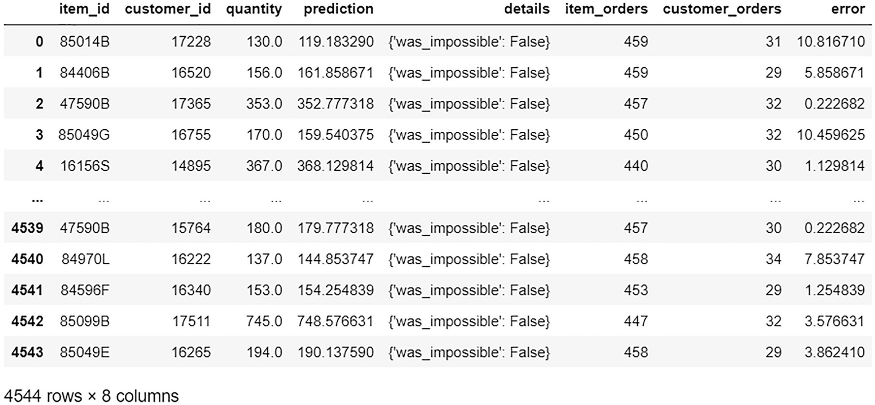
A data frame exposes the prediction data. The item id, customer id, quantity, prediction, details, item orders, customer orders, and error are represented.
Prediction DataFrame

A data frame exposes the best predictions data. The item id, customer id, quantity, prediction, details, item orders, customer orders, and error are represented.
Best predictions
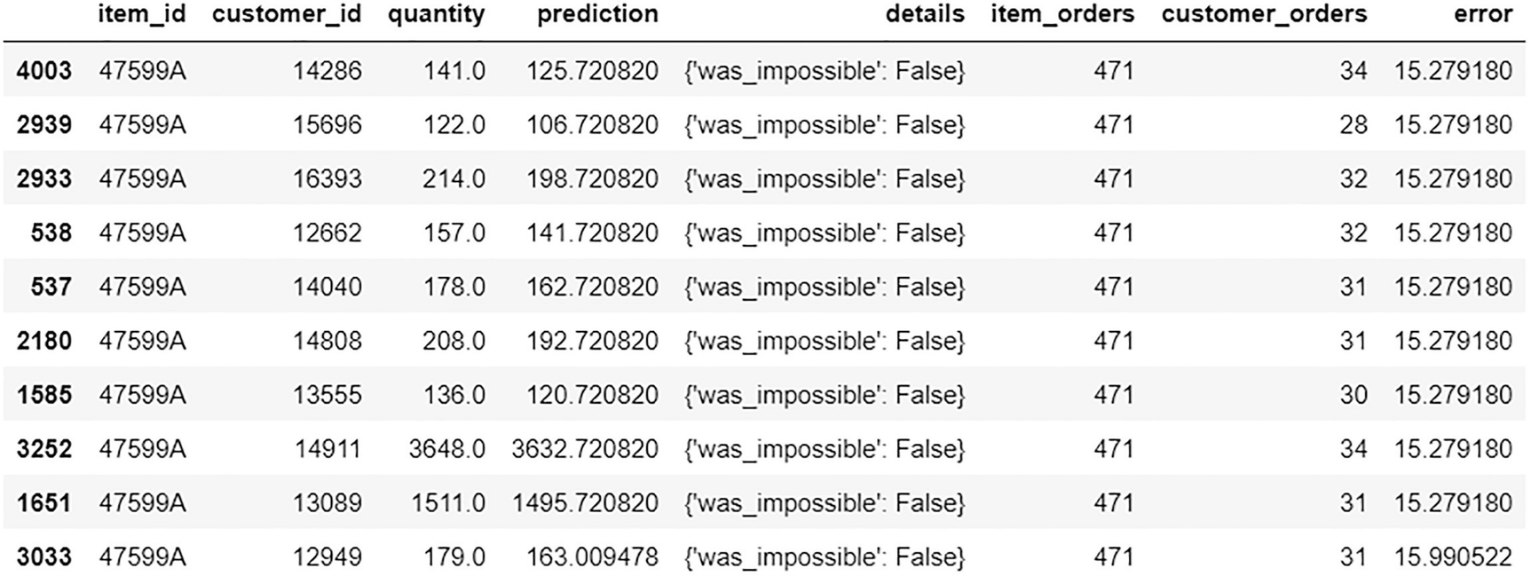
A data frame exposes the data of worst predictions. The item id, customer id, quantity, prediction, details, item orders, customer orders, and error are represented.
Worst predictions
You can now use the predictions data to get to the recommendations. First, find the customers that have bought the same items as a given user, and then from the other items they have bought, to fetch the top items and recommend them.
The recommended list of items for user 12347 is achieved.
Summary
This chapter continued the discussion of collaborative filtering-based recommendation engines. Popular methods like matrix factorization, SVD, and co-clustering were explored with a focus on implementing all three models. For the given data, the co-clustering method performed the best, but you need to try all the different methods available to see which best fits your data and use case in building a recommendation system.