
Chapter 2. Introducing core API concepts
This chapter covers
- Basics of a map in a web application
- Using different types of map data
- Performing queries
- Working with a FeatureLayer
The ArcGIS API for JavaScript is a well-stocked JavaScript library you can use to build mapping applications. In later chapters you’ll use advanced features of the API, but in this chapter I’ll discuss core features and their uses. We’ll begin our introduction to the core functions of the API with a bit of explanation about how things work so you can be better prepared when something doesn’t work as expected.
A mapping application requires you to fit together many small pieces, but the ArcGIS API for JavaScript brings all these pieces together for you, which simplifies the process. The ArcGIS API for JavaScript uses a modular approach to building web mapping applications; it loads only the necessary pieces (modules) to perform various tasks. An application that features an onscreen interactive map that you can zoom in on and pan around is remarkably simple to create. Additional functionality, such as providing user feedback or building intelligence into the application, takes more work.
To better prepare you for troubleshooting when something doesn’t work the way you expect, my approach in this chapter is to provide more in-depth explanations about how the core API functions work. I’ll cover the options that are available when you make a map, as well as the kind of data you’ll typically work with. I’ll also show you how to query your data to help you use the map to answer questions and display the results on your map. Then I’ll finish by covering the advantages of a FeatureLayer and how you can use it in your web mapping applications.
This isn’t a reference book, so I won’t cover every method and property in the ArcGIS API for JavaScript. One resource you’ll become intimately familiar with while using the API is the documentation, which you can find at https://developers.arcgis.com/en/javascript/. The API reference pages can save you time when you’re stuck on how to work with a certain module.
Esri, the company that supplies the ArcGIS API for JavaScript, also provides a collection of samples on its website that do a good job of introducing users to the basics of the API and some tools. I highly recommend these samples and reference pages, which can be found at http://esriurl.com/js, as required reading along with this book.
Now for the moment you’ve been waiting for: you’re going to dive right in and make a bare-bones mapping application. Get ready for it!
2.1. From data to map
A map is a way to visualize data. It could be basic data, such as locations of streets, or more detailed data, such as the location of census tracts. This section covers the following:
- Creating a simple map with ArcGIS API for JavaScript
- Understanding in detail the pieces that make up the map
- Reviewing common map options
Tip
Before jumping in, review appendix A to make sure you have the recommended software installed to run the samples.
First, create an HTML file using your text editor of choice, name it ch2_1.html, and enter the code shown in listing 2.1, saving it in a directory where you can view it from a local web server. Remember that to view applications built with ArcGIS API for JavaScript, the HTML files must use a local web server of your choice. Again, refer to appendix A for more information.
Listing 2.1. A simple ArcGIS JavaScript mapping application
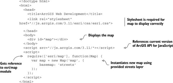
This is the minimum code you need to build a map using the ArcGIS API for JavaScript:
- A reference to the current version of the ArcGIS API for JavaScript.
- A container element, the most common of which is a div element in your HTML. A div is a block-level HTML element used for organizing your web page and can be used only within the <body> element of the page. The div element that contains the map must have a unique ID, which is associated with one element on your web page. In this case, the ID is map. You could name it Bob as long as you reference the ID correctly, but map is a convenient name for this example.
- A reference to the Esri Cascading Style Sheets (CSS) file, which defines how elements look on the page; the CSS is provided with the API to make sure the map displays correctly.
With these pieces in place, a few lines of JavaScript code are all you need to reference the esri/map module and instantiate a new instance of a map.
Definition
I use the term module to refer to individual JavaScript components that are defined in the ArcGIS API for JavaScript.
To create the map, you pass the id of the div element as the first argument to the Map constructor. This element is used to draw the map on the screen. Let’s take a look at this map in a browser.
2.1.1. Parts of a basic map
To view the results of the code in listing 2.1, run a local web server of your choice and view the HTML file in a web browser using one of the server options provided in appendix A—Visual Studio, XAMPP (Apache, MySQL, PHP), or Python:
Tip
See appendix A for viable web server options.
- Visual Studio— Right-click the HTML file and select View in Browser.
- XAMPP— Browse to http://localhost/agswebdev/ch2/ch2_1.html in your browser of choice.
- Python— From the command-line tool, navigate to the folder in which you’re saving this sample, run the command python -m SimpleHTTPServer, and navigate to http://localhost:8000/ch2_1.html in your browser.
No matter which tools you choose, you should see something similar to figure 2.1.
Figure 2.1. Your first mapping application
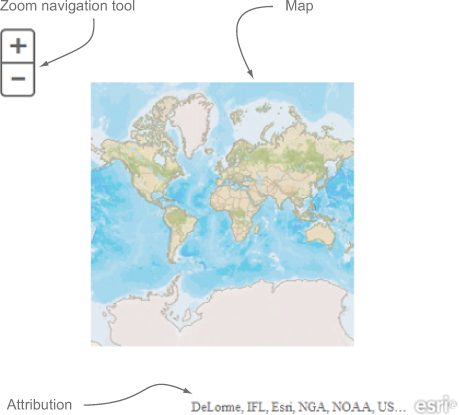
Now that’s amazing! A few lines of code and some HTML on your part, and you have a map that you can pan around and zoom in on. That’s quite the time-saver for you. Granted, this application doesn’t do much, but what do you expect from a couple of lines of code? Let’s review what you get with this basic sample. As expected, figure 2.1 is a map. Along with the map, you’re provided, by default, the attribution information in the lower-right corner. You’ll learn how to disable this attribution information at a later time, but it’s a good idea to display it so others know the source of the map information. You also have access to a navigation tool to zoom in and out of the map.
Navigating the map
I’ll talk about where this map data came from and how to change it in section 2.1.2, but first I want to point out how to navigate the map. Table 2.1 summarizes the various navigation techniques.
Table 2.1. Standard map navigation techniques
|
Technique |
Description |
|---|---|
| Left mouse-click and drag | Allows you to pan around the map |
| Mouse wheel | Zooms in and out of the map |
| Zoom navigation tool | API-provided zoom tool |
| Shift-Left mouse click and drag | Zoom shortcut |
Intuitively, you can use your mouse to left-click inside the map and pan it around. You may notice that when you pan left or right, the map keeps going. This is referred to as wrap-around, and it allows you to pan the map with a globe-like effect. It’s a neat feature if you ever need to work with the map at or near global scale.
To zoom in and out of the map, you can use the mouse wheel. The API also provides a built-in zoom navigation tool located, by default, in the upper-left area of the map. As advertised, clicking the plus (+) button zooms in; clicking the minus (−) button zooms out. One of the quickest zoom shortcuts, though, is to press the Shift key while clicking and holding the left mouse button as you move the mouse cursor over the map. You’ll notice a rectangular gray box with a red outline that represents where you’ll zoom to. You can see this preview box in figure 2.2.
Figure 2.2. Zooming with the Shift-Left mouse click shortcut displays the extent coordinates.
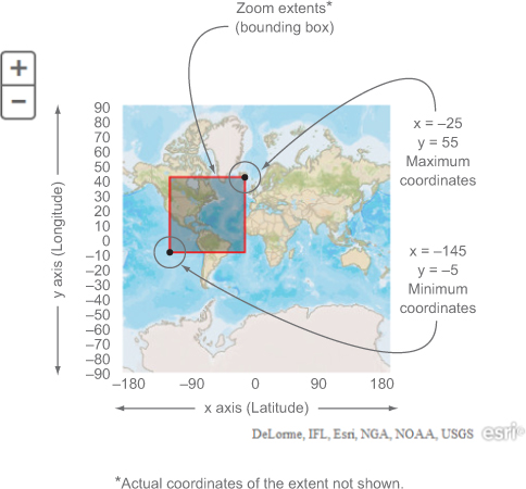
When using the Shift-Left mouse-click shortcut to zoom to a location on the map, you’re defining an extent, which the map uses to zoom in on. An extent in a mapping application is composed of a pair of x/y minimum coordinates and a pair of x/y maximum coordinates. An extent can also be referred to as a bounding box, because it’s a box that defines boundaries on a map. The lower-left coordinates of the bounding box define the minimum coordinates of an extent, and the upper-right coordinates define its maximum coordinates, as shown in figure 2.2.
When discussing map extents, it helps to cover coordinates as well.
Understanding map coordinates
Coordinates vary based on the spatial reference of the map, which I’ll discuss when I explain how to use map options, but they typically appear as shown in figure 2.2. The x axis, referred to as the longitude, runs horizontally on the globe, west to east, while the y axis, referred to as the latitude, runs vertically along the globe, north to south. Latitude at 0° and longitude at 0° is the intersection of the equator and the prime meridian. Traversing upward along the latitude yields positive coordinates, but downward yields negative coordinates. The same concept applies to the longitude: if you go west along the longitude, you get negative coordinates, and east produces positive coordinates.
Most people commonly say “x and y” to refer to latitude and longitude, but, as you can see in figure 2.2, “x and y” refers to longitude and latitude.
Don’t fret if the terminology becomes confusing. Discerning x and y and latitude and longitude can at times trip up seasoned professionals, even me.
Now let’s take another look at the JavaScript in listing 2.1 and review commonly used options that you can pass in as parameters when instantiating a new instance of a map.
2.1.2. Specifying common map options
When you created an instance of your new map, you passed it a couple of arguments:
- The id of the element on the page that contains the map
- A JavaScript object with a single value of basemap: 'streets'
The JavaScript object in the second argument contains optional parameters for creating the map. These options control the way the map is displayed when it first starts up, what type of map the user sees when it starts, where you want the map to start from, and more. When it comes to the basemap, common options, in addition to streets, include satellite, hybrid, and gray. As the parameter name suggests, this is a shortcut method to add a basemap to your application. What basemap option you choose is completely dependent on your intentions:
- streets—Provides visible information at the street level; you can see street names, and highways are easily identifiable.
- satellite and hybrid—Provides aerial images; you can see cars on freeways, the tops of buildings, and so on.
- gray—Makes the focus of the map other data, which displays on top of the map.
You don’t need to define all the options available for the map, but you should be aware of a handful of common options as you build your application. Table 2.2 lists several of the options that you can use in the parameters to construct a new map in the ArcGIS API for JavaScript. I won’t cover all the options available to pass to a map, but I’ll discuss the few that are probably used most often, such as basemap, center, and zoom.
Tip
I encourage you to review the documentation at https://developers.arcgis.com/javascript/jsapi/map.html#map1 for a full listing and explanation of all the optional parameters.
Table 2.2. Common map options
|
Option |
Description |
|---|---|
| autoResize | When set to false, the map doesn’t resize when you resize the browser. I’ve yet to find a need to set this value to false, but you never know. |
| basemap | Specifies the type of basemap the map uses by default. The options are hybrid, satellite, topo, gray, oceans, and national-geographic. |
| center | The longitude and latitude coordinates to center the map when it first starts. |
| LOD (Levels of Detail) | You can specify custom LODs for your map. A level of detail is a combination of the following:
|
| logo | When set to true, displays the Esri logo on your map. |
| nav | When set to true, displays pan arrow buttons along the edges of the map to pan in the direction of the arrow. The usefulness of this option depends on the application’s design. |
| scale | Sets the initial scale of the map when it first starts up. To focus on particular areas of the map, combine with the center option. |
| slider | When set to false, the map doesn’t display navigation tools. Other options are available to define the orientation and position of the slider navigation tools. |
| zoom | Sets the initial zoom level of the map when it first starts up. The zoom level is equal to the level value specified in an LOD. |
The next commonly used option after basemap is the center option. This is a convenient way to center your map on a specified location when the application first loads. It’s typically used in conjunction with the zoom option to also set the default zoom level of the map.
When working with the center option, note that the center coordinates you provide are in longitude and latitude, respectively, even though that may not be the spatial reference of your map. Spatial reference, in simplest terms, is the way a 3D globe of the earth is represented on a 2D map. Latitude and longitude are the most common representations of this transformation. The following code specifies the basemap, center, and zoom options for the map:
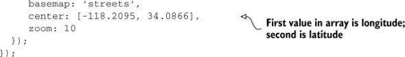
The map that results from these parameters is shown in figure 2.3.
Figure 2.3. Result of providing additional parameters for a new map
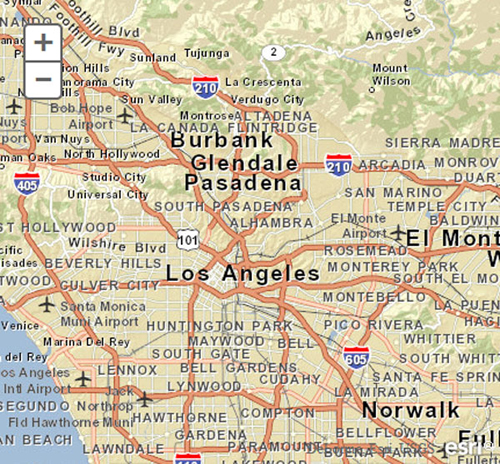
In figure 2.3, the map centers itself at the specified location and zooms in to the tenth available zoom level. A zoom level of 1 is the full global view of the map in this case; the tenth level, in addition to the coordinates you provided, zooms the map approximately to the Los Angeles County area.
So far, you’ve digested quite a bit of information about what comprises a map from the basic application you created. Now let’s dig deeper into adding layers and what layers to add.
2.2. Understanding layers and accessing data
Different types of data require different types of mapping layers to represent them. This section covers the following:
- Layer types and how they are used
- Details on vector layers
- How to use the QueryTask to display data
What you’ve seen so far by creating an instance of a map with the basemap option is an example of using a tiled service. This web mapping service aligns smaller tiled images to display a proper-looking map. This service is one type of layer you can use in your applications. A layer is a representation of geographic data displayed in your map. A simple depiction of the way layers are displayed in a map is shown in figure 2.4.
Figure 2.4. Depiction of map layers

The ArcGIS API for JavaScript provides various layer modules, some designed for specific purposes, such as KML (Keyhole Markup Language), XML-based markup (popular with Google Maps), and WMS (Web Map Services), but at the end of the day, the only difference among these services is whether the data they provide is raster- or vector-based. Raster data can be in either PNG or JPG formats; vector uses SVG (Scalable Vector Graphics), VML (Vector Markup Language), or canvas.
Note
Technically, canvas is raster-based, so it doesn’t draw vector graphics, but instead draws bitmap data. When used to render map graphics in the browser, it would be difficult to tell the difference.
2.2.1. Layer types for raster-based data
If the map you see in the web browser is a raster-based image file, it was either created ahead of time on the server or generated on an as-needed basis.
Raster data that was created ahead of time is referred to as cached data, because it’s already prepared and delivered by the server in small chunks called tiles. Data that doesn’t change often, such as streets, parcels, and aerial imagery, is cached ahead of time on the server and updated only as needed.
Raster data that’s generated on an as-needed basis is called dynamic, because the image files are created on the fly. Data that does change often is provided as dynamic data so that users always have the latest version of the data visible to them.
When to use cached or dynamic data is a decision beyond the scope of this book, but it’s still important to note what kind of map service you’re working with.
Cached data is served as an instance of an ArcGISTiledMapServiceLayer inside the ArcGIS API for JavaScript. That’s quite the mouthful, but at least it’s descriptive. To see a sample of what these tiles look like, let’s return to your bare-bones application and use the browser debugging tools in Google Chrome:
1. Press Ctrl-Shift-I (or CMD-Shift-I in Mac OS X) and then click the Network tab to see a list of all network activity in the browser.
2. Scroll the results until you see a listing of files from services.arcgisonline.com.
3. Click the image icon. You can now see a preview of an image file that was downloaded from the server.
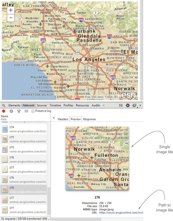
This is only one of a few image files that were downloaded, and when tiled together, they display the base data in your map, as shown in figure 2.5.
Figure 2.5. Network tools showing downloaded map images
Note
You’ll become more familiar with the Chrome DevTools as you work more with the ArcGIS API for JavaScript, especially in chapters 4 and 5. The DevTools let you view the raw HTML of the page to inspect individual HTML elements, monitor network traffic in the browser, and view what the JavaScript code is doing in real time. To learn more about Chrome DevTools, visit Code School at http://discover-devtools.codeschool.com.
Map tiles are typically 256 x 256 pixel images and are organized on the server in a specific structure:
http://<service-url>/tile/<level>/<row>/<column>
This tiling scheme is determined by the resolution of the data and the number of rows and columns that are zero-based. This means that the origin tile is located at row 0, column 0, and then you traverse right to get the next columns and down to the next rows.
Note
You can get more details about the ArcGIS Server map cache tiling scheme in the following blog posts from Esri: http://blogs.esri.com/esri/arcgis/2007/11/07/deconstructing-the-map-cache-tiling-scheme-part-i/ and http://blogs.esri.com/esri/arcgis/2008/01/31/deconstructing-the-map-cache-tiling-scheme-part-ii-working-with-map-caches-programmatically/.
The current extent of the map displayed in the browser determines which tiles are downloaded. The ArcGIS API for JavaScript sends the map’s current extent to the server, and the server determines which map tiles are needed to display the map correctly in the browser. Because individual map tiles are small, they’re cached by the browser. If you pan the map to a new location and then pan back to the previous location, these tiles don’t need to be downloaded from the server again, and because the browser caches these tiles, they load quickly.
The difference between tiled and dynamic raster data is that dynamic raster data isn’t served in tiles. The ArcGIS API for JavaScript sends a request for the current extent of the map displayed to ArcGIS Server, and ArcGIS Server returns a single image of the map that matches that extent. These dynamic images are served as an instance of the ArcGISDynamicMapServiceLayer in the API. This method isn’t as efficient, but it still serves a purpose in developing mapping applications. One such purpose is to easily display sets of data that change on a regular basis, so it wouldn’t be efficient to cache all this data ahead of time. I won’t use this layer type in this book, but it’s something you should be aware of.
HTML5 is the latest revision of the HTML standard. Most modern browsers support it—or at least support most HTML5 features. I’ll cover some of the capabilities of HTML5 in chapter 4, but when it comes to drawing graphics on a map in the ArcGIS API for JavaScript, a couple of HTML5 features are important to note. The first is SVG (Scalable Vector Graphics), which is part of HTML5 but is also a specification of its own. The HTML5 canvas element is used to draw graphics, but it doesn’t draw vector graphics. Instead, canvas draws in bitmap data, which is based on pixels.
2.2.2. Layer types for vector-based data
Vector data as it’s used in a web map is a graphical representation of geographic data in the browser. Instead of displaying images of your mapping data, vector data is displayed as graphics using x and y coordinates. Most modern browsers can display vector data using SVG, which is a standard method of displaying scalable graphics on the web. Older versions of Internet Explorer use VML, which is no longer supported in Internet Explorer 10 and above. Graphics also can be drawn using the canvas element in HTML5. VML is similar to SVG, but SVG is the current web standard for displaying vector graphics in the browser.
Browser compatibility issues plague web map development as much as any other form of web development. Luckily, the ArcGIS API for JavaScript is designed to handle these types of browser compatibility problems and use the correct vector markup as needed.
You may notice when running the code samples at home and viewing the console window in the debugging tools of your favorite browser that the following error pops up in the console:
XMLHttpRequest cannot load
http://services.arcgisonline.com/ArcGIS/rest/info?f=json. Origin
http://localhost is not allowed by Access-Control-Allow-Origin.
This error can be safely ignored in your browser. This error means that the web services are coming from a web server that isn’t CORS-enabled. CORS means cross-origin resource sharing. I won’t cover CORS in detail, but in a nutshell, it’s a browser protocol that allows servers to make requests to each other from different domains. It prevents the browser from executing JavaScript on mydomain.com from yourdomain.com, unless yourdomain.com allows it. Techniques are available to work around this from the source server, but for now, if you see this error, remember that it can be safely ignored.
The core layer that displays vector data in the ArcGIS JavaScript API is the GraphicsLayer, which is a container for various locations on the map. Locations are represented by points, lines, or polygons. Let’s look at an example to see how this works.
2.2.3. Getting to know the GraphicsLayer
Suppose you want to display a Graphic on the map at the location where the mouse was clicked. You first identify the location on the map where the mouse was clicked, and then create a Graphic to display on the map. The Graphic is a single geographic item that represents something on the map—in this case, a single coordinate on the map.
Listing 2.2 shows how to use the map.on() method to add the Graphic to the map at the location where the user clicked.
Note
The code for this section is available in the chapter2 folder of the source code included with the book. See chapter2/2.2.html and chapter2/2.2.js.
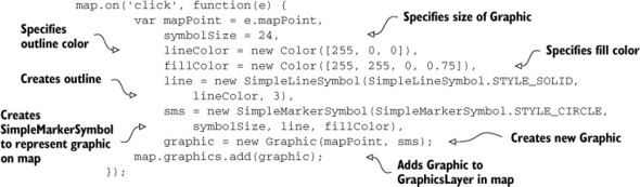
Listing 2.2. Adding a Graphic to the map
Let’s take a closer look at the map.on() method.
Identifying mouse-click location
You add map.on() after the code that defines the map variable and creates the map:
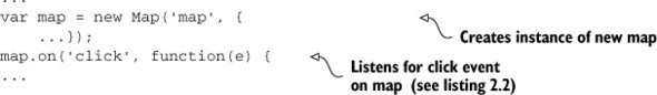
The map instance has the ability to listen for various events, such as when the mouse is clicked on the map. The map.on () method executes a function when the designated event happens. In this case, you’re waiting for a click event. As shown in listing 2.2, when a mouse-click event occurs, the ArcGIS API for JavaScript attaches a mapPoint to the event, and the mapPoint represents the location on the map that was clicked.
Creating the graphic
You designate a size in pixels for your Graphic, and specify what the Graphic looks like using other modules from the ArcGIS API for JavaScript. For example, you use the dojo/_base/Color module, which uses RGB (Red, Green, Blue) values in an array to assign a color. The fourth value in the RGB array is the transparency level for the color. You don’t want the outline to have any transparency, so omit it from the array. You want the fill color to have a 75% transparency, so set that to a value of 0.75.
When you have the outline ready using an instance of the SimpleLineSymbol, you then create a SimpleMarkerSymbol using the SimpleLineSymbol and the Color instance you created. Next, create a new Graphic using the MapPoint geometry and the SimpleMarkerSymbol. Geometry can be a point, a line, or a polygon, which are vector geometries, and in listing 2.2 you’re using a point.
The fully functional Graphic doesn’t do much until you add it to the GraphicsLayer. The map instance has a default GraphicsLayer in the map.graphics property. This property is provided so developers can easily add graphics to the map without concerning themselves with adding the GraphicsLayer manually. The resulting Graphic is shown in figure 2.6.
Figure 2.6. Adding Graphic features to the map

No matter what type of Graphic you plan on adding to a map, complete the following steps:
1. Capture geometry (a point, a line, or a polygon).
2. Define symbology (the way it looks on the map).
3. Create a new Graphic.
4. Add the Graphic to the map.
These steps may seem involved at first, but, technically, what you’ve done in this example is a prototype for a data-collection application, which is the type of application you’ll create later in the book.
In previous versions of the ArcGIS API for JavaScript, the GraphicsLayer was the only way to add graphics to the map. Typical workflow involved running a query on a map service (I’ll cover this section 2.2.4) and adding the results to a GraphicsLayer. You can still follow this workflow to display a Graphic for the user’s current location or the result of an address search, for example. Typically, you use a GraphicsLayer to display dynamic or temporary data.
At one point in the development of the ArcGIS JavaScript API, I was provided with a more robust method of working with existing data using the FeatureLayer, which I’ll cover in greater depth in section 2.3.
2.2.4. Creating graphics with the QueryTask
So far I’ve covered how to add graphics to the map by clicking locations on the map. This approach is useful in many workflows, but how would you add graphics to a map you’re not manually drawing? For example, an external map service may provide maps of river networks, point sources of emissions, or areas in danger of seasonal fires. In this scenario, you can add Graphic items to the map with the QueryTask module, which queries data in a map service. This allows you to ask the map data questions, and then you can do something with the results you’re given—for example, display the answers on a map.
QueryTask uses a Query object to define the criteria to perform this task. The Query object can have a where statement, which describes criteria for the query, such as NAME = Bob, or it can define a geometry to perform the query, as well as many other options. A query is a way of extracting data from a map service based on a defined set of criteria, such as these examples:
- Find all states that begin with “New.”
- Find all the major highways in a particular city.
To demonstrate using QueryTask, let’s embed several queries in a drop-down menu.
Creating the drop-down menu
Let’s expand on what you’ve done so far and include a drop-down menu in the HTML page (before the div element that contains the map). The following code uses a select element with option elements inside it to provide the drop-down menu:
<body>
<select id="population" name="population">
  <option value="" selected="selected">Select Population</option>
  <option value="2500">2,500</option>
  <option value="5000">5,000</option>
  <option value="7500">7,500</option>
</select>
<div id="map"></div>
</body>
When a drop-down item is selected, you use the QueryTask to retrieve the locations of census tracts that correspond to the selected population number (greater than 5,000 people, for example). So now you’re adding census tract data to the map.
Definition
According to the U.S. Census Bureau, census tracts are “small, relatively permanent statistical subdivisions of a county.”[1]
1 “American Community Survey,” U.S. Census Bureau, www.census.gov/acs/www/data_documentation/custom_tabulation_request_form/geo_def.php.
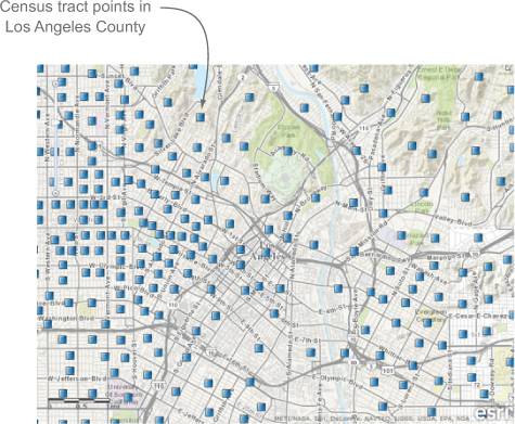
To make the census data easier to work with on the map, you’ll work with a point layer that represents the centers of each census tract in Los Angeles County. This particular layer includes labor statistics that show the population and percentage of people working in each census tract. You can see a sample of what this data looks like in figure 2.7. This is similar to what the data will look like in your application.
Figure 2.7. Census tracts in Los Angeles County represented as points
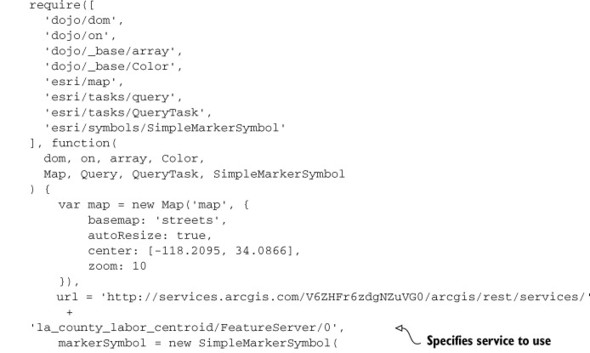
Displaying the drop-down menu results on a map
You’ll need the following modules to use the drop-down menu to filter your data:
require([
  'dojo/dom',
  'dojo/_base/array',
  'dojo/_base/Color',
  'esri/map',
  'esri/tasks/query',
  'esri/tasks/QueryTask',
  'esri/symbols/SimpleMarkerSymbol'
  ], function(
  query, array, Color,
  Map, Query, QueryTask, SimpleMarkerSymbol
) {
...
I’ve already discussed the QueryTask and the Query modules. The SimpleMarker-Symbol module defines the way the census tract points, commonly referred to as markers, appear on the map. The SimpleMarkerSymbol also needs the dojo/_base/Color module to define the color of the census tract points. For simplicity, load a helper module called dojo/_base/array, which has many utility functions for working with arrays. Table 2.3 summarizes the modules.
Table 2.3. Dojo and Esri modules needed for the drop-down filter
|
Module name |
Description |
|---|---|
| dojo/_base/array | Helper module to work with arrays |
| dojo/_base/Color | Assigns colors to Graphic |
| dojo/dom | Helper module to search elements in HTML |
| esri/map | Creates an instance of a map |
| esri/tasks/query | Defines parameters to perform searches |
| esri/symbols/SimpleMarkerSymbol | Defines how a Graphic looks on the map |
| esri/tasks/QueryTask | Queries a map service |
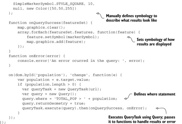
With these modules loaded, you can add this functionality to your application as shown in listing 2.3. You’ll complete the following steps:
- Instantiate your map and create a SimpleMarkerSymbol to define the appearance of the results of your QueryTask.
- Create two functions. One is used for the successful completion of a query, and the other is used, in the event of an error, to display the error message in the debug console of the browser.
- When a population number is selected from the drop-down menu, create a new QueryTask pointing to the URL of a map service, which in this case is a service that contains the census tracts as points.
- Create a new Query and define a where statement that searches for census tracts with a population greater than the population currently selected.
- Using the Query, set the returnGeometry option to true, which makes sure that the x and y coordinates of the census tract are returned with the results.
- Use the QueryTask to run an execute command (using the Query you defined) and pass along your success and error-handling functions.
When the QueryTask completes, the result you get is referred to as a FeatureSet, which is a collection of geographic data. It could contain a single point or 1,000 points; it’s only a container for this collection of data. A FeatureSet has a few properties, including the following:
- geometryType— In this case, it’s a point, but it could be a polygon or line in other situations.
- features— Contains Graphic features that represent the results of your Query.
The graphics don’t have a symbology assigned to them when you first get them, so it’s up to you to define it, which is why you made the SimpleMarkerSymbol previously in the application. You can use the array module you loaded to loop over the features, set the symbol of each Graphic to the defined symbology, and then add the Graphic to the map’s default GraphicsLayer, as shown in the following listing.
Note
The source code for this section is available in the chapter2 folder in the files chapter2/2.3.html and chapter2/2.3.js.
Listing 2.3. Add graphics with a QueryTask
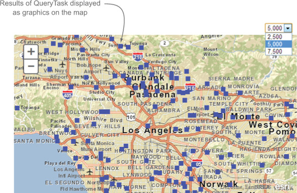
The result of this application can be seen in figure 2.8.
Figure 2.8. Displaying results of a QueryTask as graphics on the map
This small sample covers quite a bit of ground. You’re building queries to retrieve data from a map service, you’re defining the way those results are going to look, and you’re using Dojo utility modules to accomplish it all. This represents a pattern you’ll see often in developing your web mapping applications:
- Perform a query
- Handle query results
- Display results on a map
The QueryTask is a commonly used tool in your ArcGIS API for JavaScript toolbox. Before I cover the next powerful tool, the FeatureLayer, review table 2.4, which summarizes the key terms I covered in this section.
Table 2.4. Key raster, vector, and GraphicsLayer terms
|
Term |
Description |
|---|---|
| FeatureSet | A collection of features returned as a result from performing a query on a map service |
| Graphic | Used to represent vector geometries on the map |
| GraphicsLayer | Layer in the map that contains various Graphic items to display data on the map |
| Map tiles | 256 x 256 image tiles used to represent static map data |
| QueryTask | Module provided in the JavaScript API to perform queries on map services |
| Raster data | Nonvector data represented as an image in the browser |
| Symbology | How a Graphic is displayed on the map, such as by color, size, and opacity |
| Vector data | Geometries such as points, lines, or polygons displayed on the map |
The FeatureLayer in the ArcGIS API for JavaScript is a combination of a GraphicsLayer and a QueryTask.
2.3. Working with the FeatureLayer
The FeatureLayer was added to the API to provide a more robust method of working with vector data. It provides various methods to display vector data on the map in an efficient manner. You’d use a GraphicsLayer to display fire hydrants on a street, but you’d use a FeatureLayer to add new fire hydrants to the map.
The FeatureLayer is a robust module in the API because it acts as a GraphicsLayer for a layer in a map service and also provides editing capabilities, which I’ll cover in chapters 4 and 5. Because it also includes a built-in QueryTask, it can be used to select items from itself.
For now, let’s discuss how the FeatureLayer can display data from a single layer in a map service or a feature service. I’ll cover a feature service, which is a service that allows you to edit data, more extensively in chapter 4. This section covers many things, so here’s a brief overview:
- I’ll cover some of the reasons you would use a FeatureLayer and what advantages it provides to you as a developer.
- Then I’ll discuss how to create a FeatureLayer and the various options that are available to you.
- I’ll also cover what modes are available for a FeatureLayer, as well as how to create a DefinitionExpression.
- I’ll wrap up the discussion of the FeatureLayer by looking at how to perform a spatial query in which you select items in the FeatureLayer using a geometry that you define.
2.3.1. Advantages of a FeatureLayer
When you first start working with a FeatureLayer, you may wonder why you shouldn’t use the GraphicsLayer to display data on the map. A FeatureLayer is a combination of a GraphicsLayer and a QueryTask, so what makes it so special? The FeatureLayer has optimizations built into it that make displaying large datasets faster and more efficient than trying to manage it on your own with a GraphicsLayer.
Performing generalizations
A FeatureLayer is designed to request only the data that matters. Browser real estate is measured in pixels. The resolution of a map can be measured by specifying that “one pixel equals [a certain distance on the map].” Depending on the zoom level, this distance could be 100 miles or 100 feet. The FeatureLayer sends this information to the map server. The server then determines whether more than one vertex of a line or polygon is displayed in a pixel. If so, it returns a single vertex instead of the dozen or so vertices that might be there. This process is called generalization. The browser would be unable to draw the Graphic features at any finer detail anyway, so for larger data-sets, this makes quite a difference in the download size of the data returned from the server. It can make the difference between returning a 2-megabyte file and a 200-kilobyte file, which you’d definitely notice (see figure 2.9).
Figure 2.9. How a FeatureLayer might be generalized to optimize the data
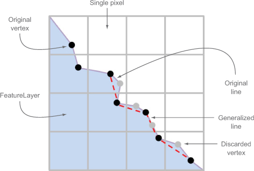
In figure 2.9 you can see that if a single pixel contains multiple vertices, the server returns only one vertex per pixel.
The generalization setting in a FeatureLayer is automatic, but you can disable it or set it manually:
To disable generalization—Set the autoGeneralization option to false in the constructor for a FeatureLayer.
To manually set generalization—Specify an offset using setMaxAllowableOffset with the FeatureLayer.
I haven’t run across a case in which I’ve needed to do this; however, if you’re working on a large dataset that still loads slowly with the default options, you can rest easy knowing that these options can be changed.
Using vector tiles
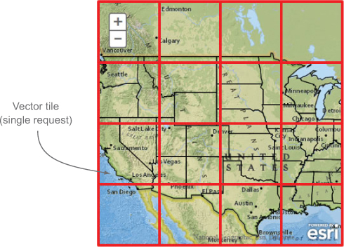
Another great feature you get with FeatureLayers is the use of vector tiling. I discussed image map tiles previously (see section 2.2), and vector tiles work in a similar manner. By default, when data is requested to be used in a FeatureLayer, it’s requested in chunks. These chunks are defined by a virtual grid of the current map extents. So instead of making a single request for all the data currently in the map extents, it makes multiple requests for smaller sections of the map to display all the features. You can see an example of how this might look in figure 2.10.
Figure 2.10. How vector tiles might be requested for a map
Vector tiling is the default behavior of a FeatureLayer and is described as “on-demand” mode. A few modes are available for a FeatureLayer, and I’ll discuss those in section 2.3.3, but with the on-demand mode, the data is requested only as needed.
Another benefit of vector tiling is that the data is cached in the browser, so when panning the map around, if the web application requests a vector tile from the server that was previously provided, the server tells the application to get the data from the cache. This optimization allows the FeatureLayer to take advantage of the browser cache to increase performance of the web application.
Now that I’ve talked about the advantages of a FeatureLayer, let’s move on to creating a map with it.
2.3.2. Creating a FeatureLayer
To add a FeatureLayer to the map, create a new instance of a FeatureLayer with a source URL and add it to the map:
var featureLayer = new FeatureLayer(
  'http://services.arcgis.com/' +
  'V6ZHFr6zdgNZuVG0/arcgis/rest/services' +
  '/la_county_labor_centroid/FeatureServer/0'
);
map.addLayer(featureLayer);
With a couple of lines of code, you can load this entire layer of graphics into your map, as shown in figure 2.11.
Figure 2.11. Graphics displayed in a map using a FeatureLayer

What you see in figure 2.11 are numerous points displayed as Graphic features on the map. By default, the FeatureLayer renders items on the map as they were designed when the source data was defined; it uses the same symbols used in the desktop software that created the data. In this case, instead of being an SVG element on the map, it’s displaying an image for each point on the map internally, using a SimplePictureMarkerSymbol from the ArcGIS API for JavaScript. The SimplePictureMarkerSymbol allows you to use an image instead of an SVG graphic to represent a location on the map.
If you use a debugging tool like the tools built into Google Chrome and inspect the map element, you’ll see that the GraphicsLayer is composed of thousands of images using Base64-encoded image data (see figure 2.12). I’ll cover Base64-encoded image data in the next chapter.
Figure 2.12. Inspecting HTML to see how FeatureLayer provides data

As you can see from the number of features shown in figure 2.12, this is a large amount of data for the map to display. Too much data can significantly impact the performance of your application. In this case, even though this image is fairly small, the browser still uses up memory to draw it on the screen.
2.3.3. Optimizing application performance
To manage your application’s performance, you can set different modes for the FeatureLayer:
- MODE_SNAPSHOT— Retrieves all data from the service and displays it on the map. My suggestion is to use this one sparingly as it can heavily impact map performance. This mode is best suited for a service that provides minimal data, such as a jurisdictional boundary.
- MODE_ONDEMAND— Retrieves only data from the service that’s in the current extent of the map.
- MODE_SELECTION— Retrieves only data from the service when the data is selected using a query.
I won’t cover MODE_SNAPSHOT, as it downloads all the data, and you have quick access to it. This could impact the performance of your application if it tries to download a large amount of data. It’s best used for smaller bits of data and also prevents the application from retrieving data from the server unnecessarily.
Using a DefinitionExpression
By default, the FeatureLayer uses MODE_ONDEMAND. In the case of this example, this retrieves almost all the data in the feature service, which is why it may not perform well. To make working with large amounts of data in the FeatureLayer more manageable, you’ll define a DefinitionExpression—a set of criteria you can define on the FeatureLayer to limit the data that’s retrieved.
This particular feature service includes population information for census tracts, so you may want to display only locations with a population greater than 5,000 people. You can do this by setting the DefinitionExpression on the FeatureLayer:
featureLayer.setDefinitionExpression('TOTAL_POP > 5000'),
When you do this, you can see in figure 2.13 that the map displays markedly less data.
Figure 2.13. FeatureLayer with DefinitionExpression of 'TOTAL_POP > 5000' applied
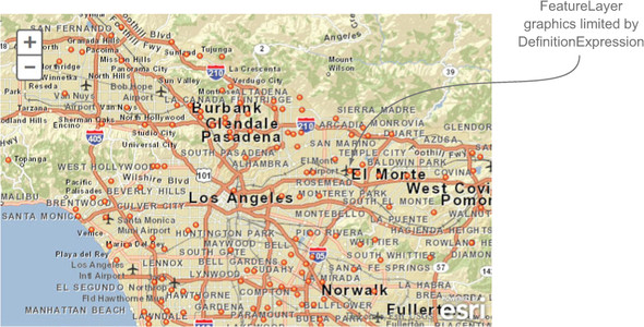
The FeatureLayer is still in on-demand mode, but now it limits the amount of data requested by the criteria you set in the DefinitionExpression. This combination can greatly improve performance of your application.
Now you’re starting to do something more interesting with your data. By providing a DefinitionExpression, you’re asking the data questions and displaying the response. Let’s make this application even more interactive.
Using a dynamic DefinitionExpression
Let’s add a menu that allows users to filter the data by a specific population range. To create the menu, add a select HTML element with options to your page (found in the chapter 2 folder in the 2.4.html file) as you did with the GraphicsLayer previously:
<body>
    <select id="population" name="population">
      <option value="2500" selected="selected">2,500</option>
      <option value="5000">5,000</option>
      <option value="7500">7,500</option>
    </select>
    <div id="map"></div>
  </body>
Now that you’ve modified your HTML page, let’s look at the JavaScript (the 2.4.js file of the source code) that makes everything work, as shown in the following listing.
Listing 2.4. JavaScript for simple filter application
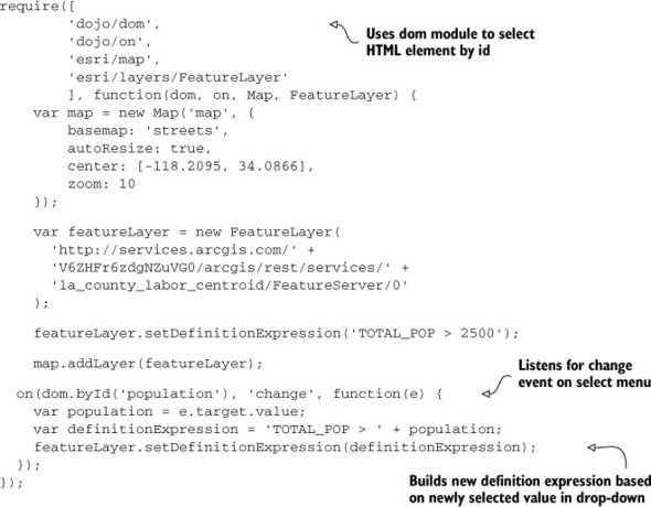
You’re now interacting with the map to update the data displayed on the map. This example is starting to look more like a functioning application. The newly updated application is shown in figure 2.14.
Figure 2.14. Interactive map application using a DefinitionExpression
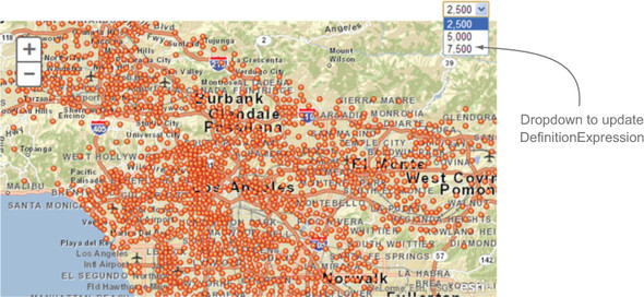
Working with the DefinitionExpression in a FeatureLayer is an elegant yet powerful way to interact with your data. Previously I mentioned that a FeatureLayer is a combination of a GraphicsLayer and query functionality. It’s that built-in query functionality that allows you to interact with the FeatureLayer by selecting features, which I’ll cover next.
2.3.4. Selecting items in the FeatureLayer
Another method of using the FeatureLayer is to use it in MODE_SELECTION. In MODE_SELECTION, you don’t set a DefinitionExpression because the data that’s retrieved from the server is retrieved using the FeatureLayer.selectFeatures() method. This works similarly to the DefinitionExpression, in which you define a set of criteria to filter your data, but you gain more flexibility. One of the main benefits of using MODE_SELECTION is that you can filter the data by a spatial geometry, such as a polygon.
In MODE_SELECTION, the FeatureLayer doesn’t display any data when it first loads. It’s up to you to define the criteria to do the selection. In this example we’ll draw a polygon on the map and use that polygon to select items in the FeatureLayer. The HTML page looks similar to the previous example except that you click a button on the page to activate a drawing tool and begin drawing on the map:
...
<body>
     <input name="drawPolygon" type="button" id="drawPolygon" value="Draw"/>
     <div id="map"></div>
</body>
...
Your JavaScript (see listing 2.5) introduces a new module in the ArcGIS API for JavaScript, the Draw toolbar, which allows you to draw graphics on your map. The result of a completed drawing is an event that contains the geometry that was drawn on the map. The geometry could be a point, line, or polygon, but the key is that you use this geometry to perform a spatial query on your FeatureLayer. A spatial query is a way to filter data by spatial means, such as a polygon.
Listing 2.5. JavaScript to perform a FeatureLayer selection


The result of this code is shown in figure 2.15.
Figure 2.15. Drawing a polygon (at left) to select features in a FeatureLayer (at right)
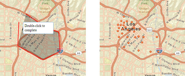
As shown in figure 2.15, when you query a FeatureLayer using the geometry from the DrawToolbar, it displays only the features that are inside that geometry, which gives this example a lot of power.
Table 2.5 summarizes the FeatureLayer-related terms that I covered in this section.
Table 2.5. Key FeatureLayer terms
|
Term |
Description |
|---|---|
| DefinitionExpression | A set of criteria you can set on a layer to limit the data shown on the map |
| FeatureLayer | Optimized layer that works with vector data on the map |
| Generalization | A method of optimizing vector data to reduce the amount of data needed to display on the map |
| Modes | Various modes that you can set on a FeatureLayer to determine how it’s used in the map |
| Vector tiles | An optimized method of requesting vector data as a virtual grid and taking advantage of the browser cache |
The ability to filter features in a map based on geometry is one of the most common use cases in developing mapping applications. Imagine that a researcher wants to restrict an analysis to a particular area or that an engineer wants to extract only manholes in a particular service area. Filtering spatial data is a cornerstone of GIS analysis and a feature that proves useful in a web application.
2.4. Summary
- The ArcGIS API for JavaScript is an extensive collection of modules that provide a full suite of tools to build powerful mapping applications. It would be impossible to cover every module in depth without this book becoming a reference manual, but the goal here is to provide information on how to get the pieces to fit together. The topics covered in this chapter provide a solid foundation in understanding how a map is displayed in the browser and the types of data that can be used.
- I covered tiled services and vector graphics in the map, but you could display numerous other types of data, such as a WMSLayer (Web Map Services), a KMLLayer (XML-based format popular with Google Maps), or a WebTiledLayer (generic layer to load nonArcGIS Server tiles), which I didn’t cover.
- You learned how to use a GraphicsLayer to display data on a map and how to use a FeatureLayer to not only display your data but also perform queries on that data.
In chapter 3 you’ll become more familiar with how to interact with the ArcGIS Server through the ArcGIS Server REST API.