7

Deep Learning with Neural Networks

Learning Objectives

By the end of this chapter, you will be able to:

• Perform basic TensorFlow operations to solve various expressions
• Describe how aritifical neural networks work
• Train and test neural networks with TensorFlow
• Implement deep learning neural network models with TensorFlow

In this chapter, we'll detect a written digit using the TensorFlow library.

Introduction

In this chapter, we will learn about another supervised learning technique. However, this time, instead of using a simple mathematical model such as classification or regression, we will use a completely different model: neural networks. Although we will use Neural Networks for supervised learning, note that Neural Networks can also model unsupervised learning techniques. The significance of this model increased in the last century, because in the past, the computation power required to use this model for supervised learning was not enough. Therefore, neural networks have emerged in practice in the last century.

TensorFlow for Python

TensorFlow is one of the most important machine learning and open source libraries maintained by Google. The TensorFlow API is available in many languages, including Python, JavaScript, Java, and C. As TensorFlow supports supervised learning, we will use TensorFlow for building a graph model, and then use this model for prediction.

TensorFlow works with tensors. Some examples for tensors are:

• Scalar values such as a floating point number.
• A vector of arbitrary length.
• A regular matrix, containing p times q values, where p and q are finite integers.
• A p x q x r generalized matrix-like structure, where p, q, r are finite integers. Imagine this construct as a rectangular object in three dimensional space with sides p, q, and r. The numbers in this data structure can be visualized in three dimensions.
• Observing the above four data structures, more complex, n-dimensional data structures can also be valid examples for tensors.

We will stick to scalar, vector, and regular matrix tensors in this chapter. Within the scope of this chapter, think of tensors as scalar values, or arrays, or arrays of arrays.

TensorFlow is used to create artificial neural networks because it models its inputs, outputs, internal nodes, and directed edges between these nodes. TensorFlow also comes with mathematical functions to transform signals. These mathematical functions will also come handy when modeling when a neuron inside a neural network gets activated.

Note

Tensors are array-like objects. Flow symbolizes the manipulation of tensor data. So, essentially, TensorFlow is an array data manipulation library.

The main use case for TensorFlow is artificial neural networks, as this field requires operation on big arrays and matrices. TensorFlow comes with many deep learning-related functions, and so it is an optimal environment for neural networks. TensorFlow is used for voice recognition, voice search, and it is also the brain behind translate.google.com. Later in this chapter, we will use TensorFlow to recognize written characters.

Installing TensorFlow in the Anaconda Navigator

Let's open the Anaconda Prompt and install TensorFlow using pip:

pip install tensorflow

Installation will take a few minutes because the package itself is quite big. If you prefer using your video card GPU instead of your CPU, you can also use tensorflow-gpu. Make sure that you only use the GPU version if you have a good enough graphics card for it.

Once you are done with the installation, you can import TensorFlow in IPython:

import tensorflow as tf

First, we will use TensorFlow to build a graph. The execution of this model is separated. This separation is important because execution is resource intensive and may therefore run on a server specialized in solving computation heavy problems.

TensorFlow Operations

TensorFlow provides many operations to manipulate data. A few examples of these operations are as follows:

• Arithmetic operations: add and multiply
• Exponential operations: exp and log
• Relational operations: greater, less, and equal
• Array operations: concat, slice, and split
• Matrix operations: matrix_inverse, matrix_determinant, and matmul
• Neural network-related operations: sigmoid, ReLU, and softmax

Exercise 22: Using Basic Operations and TensorFlow constants

Use arithmetic operations in Tensorflow to solve the expression: 2 * 3 + 4

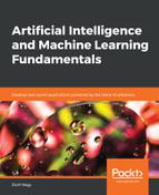
These operations can be used to build a graph. To understand more about TensorFlow constants and basic arithmetic operators, let's consider a simple expression 2 * 3 + 4 the graph for this expression would be as follows:

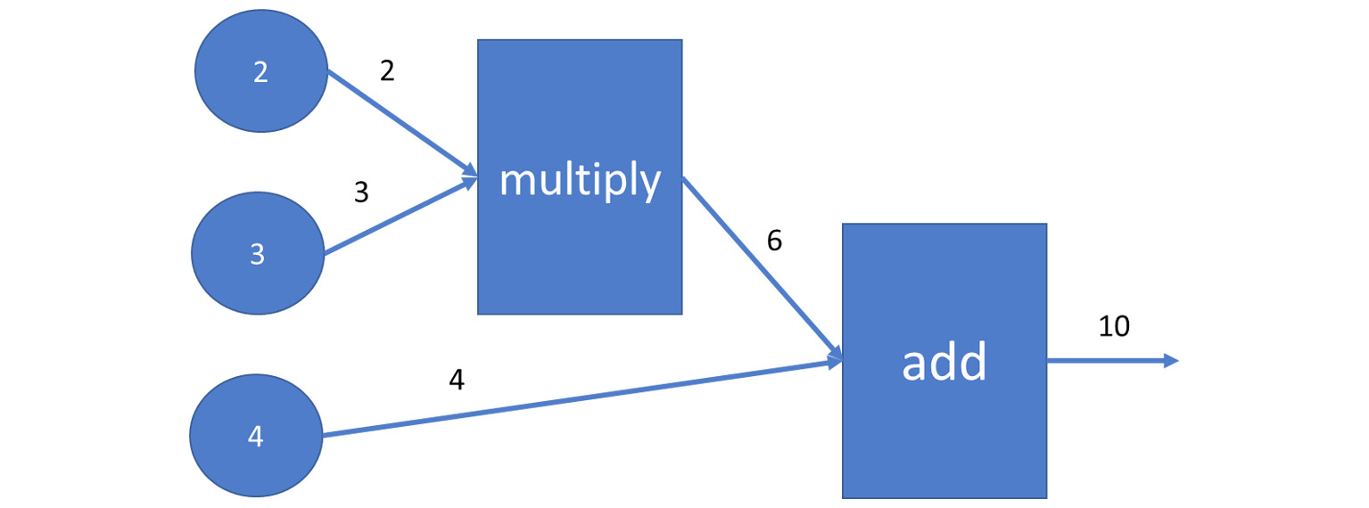
Figure 7.1: Graph of the expression 2*3+4

1. Model this graph in TensorFlow by using the following code:

   import tensorflow as tf

   input1 = tf.constant(2.0, tf.float32, name='input1')

   input2 = tf.constant(3.0, tf.float32, name='input2')

   input3 = tf.constant(4.0, tf.float32, name='input3')

   product12 = tf.multiply(input1, input2)

   sum = tf.add(product12, input3)

2. Once the graph is built, to perform calculations, we have to open a TensorFlow session and execute our nodes:

   with tf.Session() as session:

       print(session.run(product12))

       print(session.run(sum))

   The intermediate and final results are printed to the console:

   6.0

   10.0

Placeholders and Variables

Now that you can build expressions with TensorFlow, let's take things a step further and build placeholders and variables.

Placeholders are substituted with a constant value when the execution of a session starts. Placeholders are essentially parameters that are substituted before solving an expression. Variables are values that might change during the execution of a session.

Let's create a parametrized expression with TensorFlow:

import tensorflow as tf

input1 = tf.constant(2.0, tf.float32, name='input1')

input2 = tf.placeholder(tf.float32, name='p')

input3 = tf.Variable(0.0, tf.float32, name='x')

product12 = tf.multiply(input1, input2)

sum = tf.add(product12, input3)

with tf.Session() as session:

    initializer = tf.global_variables_initializer()

    session.run(initializer)

    print(session.run(sum, feed_dict={input2: 3.0}))

The output is 6.0.

The tf.global_variables_initializer() call initialized the variable in input3 to its default value, zero, after it was executed in session.run.

The sum was calculated inside another session.run statement by using the feed dictionary, thus using the constant 3.0 in place of the input2 parameter.

Note that in this specific example, the variable x is initialized to zero. The value of x does not change during the execution of the TensorFlow session. Later, when we will use TensorFlow to describe neural networks, we will define an optimization target, and the session will optimize the values of the variables to meet this target.

Global Variables Initializer

As TensorFlow often makes use of matrix operations, it makes sense to learn how to initialize a matrix of random variables to a value that's randomly generated according to a normal distribution centered at zero.

Not only matrices, but all global variables are initialized inside the session by calling tf.global_variables_initializer():

randomMatrix = tf.Variable(tf.random_normal([3, 4]))

with tf.Session() as session:

    initializer = tf.global_variables_initializer()

    print( session.run(initializer))

    print( session.run(randomMatrix))

    

None

[[-0.41974232 1.8810892 -1.4549098 -0.73987174]

[ 2.1072254 1.7968426 -0.38310152 0.98115194]

[-0.550108 -0.41858754 1.3511614 1.2387075 ]]

As you can see, the initialization of a tf.Variable takes one argument: the value of tf.random_normal([3,4]).

Introduction to Neural Networks

Neural networks are the newest branch of AI. Neural networks are inspired by how the human brain works. Originally, they were invented in the 1940s by Warren McCulloch and Walter Pitts. The neural network was a mathematical model that was used for describing how the human brain can solve problems.

We will use the phrase artificial neural network when talking about the mathematical model and use biological neural network when talking about the human brain. Artificial neural networks are supervised learning algorithms.

The way a neural network learns is more complex compared to other classification or regression models. The neural network model has a lot of internal variables, and the relationship between the input and output variables may go through multiple internal layers. Neural networks have higher accuracy as compared to other supervised learning algorithms.

Note

Mastering neural networks with TensorFlow is a complex process. The purpose of this section is to provide you with an introductory resource to get started.

In this chapter, the main example we are going to use is the recognition of digits from an image. We are considering this image since it is small, and we have around 70,000 images available. The processing power required to process these images, is similar to that of a regular computer.

Artificial neural network works similar to human brain works. Dendroid in a human brain is connected to the nucleus and the nucleus is connected to the axon. Here, the dendroid acts as the inputs, nucleus is where the calculations occurs (weighted sum and the activation function) and the axon acts similar to the output.

Then, we determine which neuron fires by passing the weighted sum to an activation function. If this function determines that a neuron has to fire, the signal appears in the output. This signal can be the input of other neurons in the network:

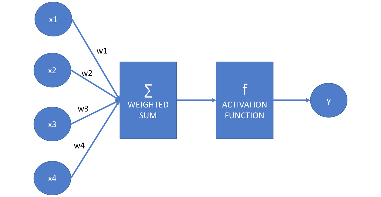
Figure 7.2: Diagram showing how the artificial neural network works

Suppose f is the activation function, x1, x2, x3, and x4 are the inputs, and their sum is weighted with the weights w1, w2, w3, and w4:

y = f(x1*w1 + x2*w2 + x3*w3 + x4*w4)

Assuming vector x is (x1, x2, x3, x4) and vector w is (w1, w2, w3, w4), we can write this equation as the scalar or dot product of these two vectors:

y = f(x ⋅ w)

The construct we have defined is one neuron:

Let's hide the details of this neuron so that it becomes easier to construct a neural network:

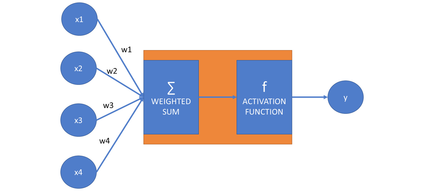
Figure 7.4: Diagram that represents the hidden layer of a neuron

We can create multiple boxes and multiple output variables that may get activated as a result of reading the weighted average of inputs.

Although in the following diagram there are arrows leading from all inputs to all boxes, bear in mind that the weights on the arrows might be zero. We still display these arrows in the diagram:

Figure 7.5: Diagram representing a neural network

The boxes describing the relationship between the inputs and the outputs are referred to as a hidden layer. A neural network with one hidden layer is called a regular neural network.

When connecting inputs and outputs, we may have multiple hidden layers. A neural network with multiple layers is called a deep neural network:

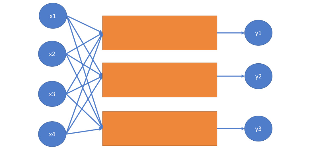
Figure 7.6: A diagram representing a deep neural network

The term deep learning comes from the presence of multiple layers. When creating an artificial neural network, we can specify the number of hidden layers.

Biases

Let's see the model of a neuron in a neural network again:

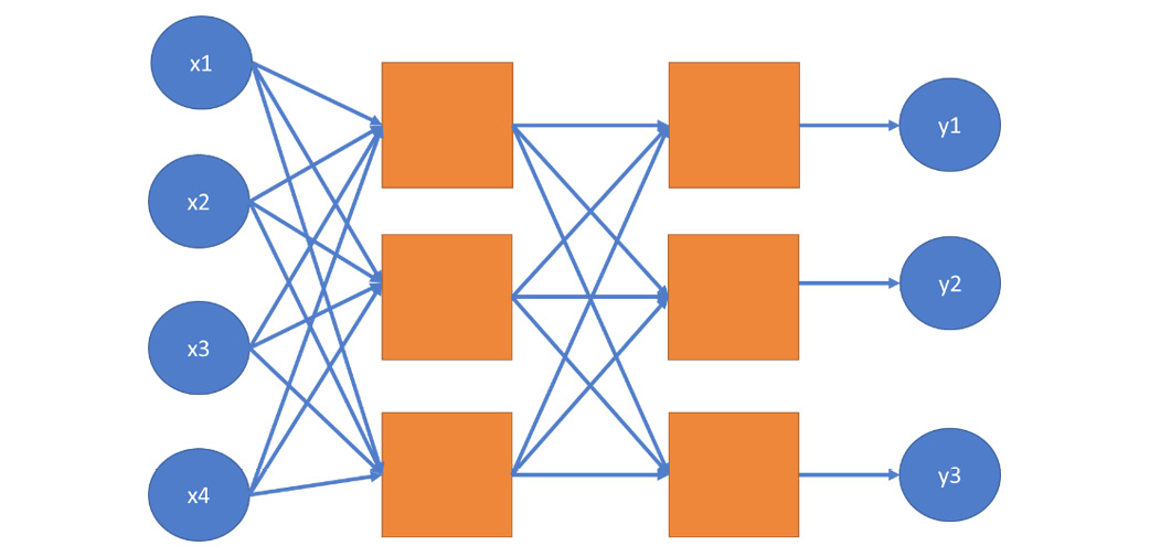
Figure 7.7: Diagram of neuron in neural network

We learned that the equation of this neuron is as follows:

y = f(x1*w1 + x2*w2 + x3*w3 + x4*w4)

The problem with this equation is that there is no constant factor that depends on the inputs x1, x2, x3, and x4. This implies that each neuron in a neural network, without bias, always produces this value whenever for each weight-input pair, their product is zero.

Therefore, we add bias to the equation:

y = f(x1*w1 + x2*w2 + x3*w3 + x4*w4 + b)

y = f(x ⋅ w + b)

The first equation is the verbose form, describing the role of each coordinate, weight coefficient, and bias. The second equation is the vector form, where x = (x1, x2, x3, x4) and w = (w1, w2, w3, w4). The dot operator between the vectors symbolizes the dot or scalar product of the two vectors. The two equations are equivalent. We will use the second form in practice because it is easier to define a vector of variables using TensorFlow than to define each variable one by one.

Similarly, for w1, w2, w3, and w4, the bias b is a variable, meaning that its value can change during the learning process.

With this constant factor built into each neuron, the neural network model becomes more flexible from the purpose of fitting a specific training dataset better.

Note

It may happen that the product p = x1*w1 + x2*w2 + x3*w3 + x4*w4 is negative due to the presence of a few negative weights. We may still want to give the model the flexibility to fire a neuron with values above a given negative number. Therefore, adding a constant bias b = 5, for instance, can ensure that the neuron fires for values between -5 and 0 as well.

Use Cases for Artificial Neural Networks

Artificial neural networks have their place among supervised learning techniques. They can model both classification and regression problems. A classifier neural network seeks a relationship between features and labels. The features are the input variables, while each class the classifier can choose as a return value is a separate output. In the case of regression, the input variables are the features, while there is one single output: the predicted value. While traditional classification and regression techniques have their use cases in artificial intelligence, artificial neural networks are generally better at finding complex relationships between the inputs and the outputs.

Activation Functions

Different activation functions are used in neural networks. Without these functions, the neural network would be a linear model that could be easily described using matrix multiplication.

Activation functions of the neural network provide non-linearity. The most common activation functions are sigmoid and tanh (the hyperbolic tangent function).

The formula of sigmoid is as follows:

import numpy as np

def sigmoid(x):

    return 1 / (1 + np.e ** (-x))

Let's plot this function using pyplot:

import matplotlib.pylab as plt

x = np.arange(-10, 10, 0.1)

plt.plot(x, sigmoid(x))

plt.show()

The output is as follows:

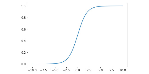
Figure 7.8: Graph displaying the sigmoid curve

There are a few problems with the sigmoid function.

First, it may disproportionally amplify or dampen weights.

Second, sigmoid(0) is not zero. This makes the learning process harder.

The formula of the hyperbolic tangent is as follows:

def tanh(x):

    return 2 / (1 + np.e ** (-2*x)) - 1

We can also plot this function like so:

x = np.arange(-10, 10, 0.1)

plt.plot(x, tanh(x))

plt.show()

The output is as follows:

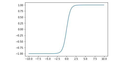
Figure 7.9: Graph after plotting hyperbolic tangent

Both functions add a little non-linearity to the values emitted by a neuron. The sigmoid function looks a bit smoother, while the tanh function gives slightly more edgy results.

Another activation function has become popular lately: ReLU. ReLU stands for Rectified Linear Unit:

def relu(x):

    return 0 if x < 0 else x

Making the neural network model non-linear makes it easier for the model to approximate non-linear functions. Without these non-linear functions, regardless of the number of layers of the network, we would only be able to approximate linear problems:

def reluArr(arr):

   return [relu(x) for x in arr]

x = np.arange(-10, 10, 0.1)

plt.plot(x, reluArr(x))

plt.show()

The output is as follows:

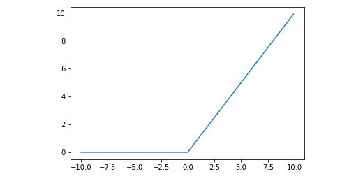
Figure 7.10: Graph displaying the ReLU function

The ReLU activation function behaves surprisingly well from the perspective of quickly converging to the final values of the weights and biases of the neural network.

We will use one more function in this chapter: softmax.

The softmax function shrinks the values of a list between 0 and 1 so that the sum of the elements of the list becomes 1. The definition of the softmax function is as follows:

def softmax(list):

    return np.exp(list) / np.sum(np.exp(list))

Here is an example:

softmax([1,2,1])

The output is as follows:

array([0.21194156, 0.57611688, 0.21194156])

The softmax function can be used whenever we filter a list, not a single value. Each element of the list will be transformed.

Let's experiment with different activator functions. Observe how these functions dampen the weighted inputs by solving the following exercise.

Exercise 23: Activation Functions

Consider the following neural network:

y = f( 2 * x1 + 0.5 * x2 + 1.5 * x3 - 3 ).

Assuming x1 is 1 and x2 is 2, calculate the value of y for the following x values: -1, 0, 1, 2, when:

• f is the sigmoid function
• f is the tanh function
• f is the ReLU function

Perform the following steps:

1. Substitute the known coefficients:

   def get_y( f, x3 ):

       return f(2*1+0.5*2+1.5*x3)

2. Use the following three activator functions:

   import numpy as np

   def sigmoid(x):

       return 1 / (1 + np.e ** (-x))

   def tanh(x):

       return 2 / (1 + np.e ** (-2*x)) - 1

   def relu(x):

       return 0 if x < 0 else x

3. Calculate the sigmoid values, using the following commands:

   get_y( sigmoid, -2 )

   The output is 0.5

   get_y(sigmoid, -1)

   The output is 0.8175744761936437

   get_y(sigmoid, 0)

   The output is 0.9525741268224331

   get_y(sigmoid, 1)

   The output is 0.9890130573694068

   get_y(sigmoid, 2)

   The output is 0.9975273768433653

4. As you can see, the changes are dampened quickly as the sum of the expression inside the sigmoid function increases. We expect the tanh function to have an even bigger dampening effect:

   get_y(tanh, -2)

   The output is 0.0

   get_y(tanh, -1)

   The output is 0.9051482536448663

   get_y(tanh, 0)

   The output is 0.9950547536867307

   get_y(tanh, 1)

   The output is 0.9997532108480274

   get_y(tanh, 2)

   The output is 0.9999877116507956

5. Based on the characteristics of the tanh function, the output approaches the 1 asymptote faster than the sigmoid function. For x3 = -2, we calculate f(0). While sigmoid(0) is 0.5, tanh(0) is 0. As opposed to the other two functions, the ReLu function does not dampen positive values:

   get_y(relu,-2)

   The output is 0.0

   get_y(relu,-1)

   The output is 1.5

   get_y(relu,0)

   The output is 3.0

   get_y(relu,1)

   The output is 4.5

   get_y(relu,2)

   The output is 6.0

   Another advantage of the ReLU function is that its calculation is the easiest out of all of the activator functions.

Forward and Backward Propagation

As artificial neural networks provide a supervised-learning technique, we have to train our model using training data. Training the network is the process of finding the weights belonging to each variable-input pair. The process of weight optimization consists of the repeated execution of two steps: forward propagation and backward propagation.

The names forward and backward propagation imply how these techniques work. We start by initializing the weights on the arrows of the neural network. Then, we apply forward propagation, followed by backward propagation.

Forward propagation calculates output values based on input values. Backward propagation adjusts the weights and biases based on the margin of error measured between the label values created by the model and the actual label values in the training data. The rate of adjustment of the weights depend on the learning rate of the neural network. The higher the learning rate, the more the weights and biases are adjusted during the backward propagation. The momentum of the neural network determines how past results influence the upcoming values of weights and biases.

Configuring a Neural Network

The following parameters are commonly used to create a neural network:

• Number of hidden layers
• Number of nodes per hidden layer
• Activation function
• Learning rate
• Momentum
• Number of iterations for forward and backward propagation
• Tolerance for error

There are a few rules of thumb that can be used to determine the number of nodes per hidden layer. If your hidden layer contains more nodes than the size of your input, you risk overfitting the model. Often, a node count somewhere between the number of inputs and the number of outputs is reasonable.

Importing the TensorFlow Digit Dataset

Recognition of hand-written digits seems to be a simple task at first glance. However, this task is a simple classification problem with ten possible label values. TensorFlow provides an example dataset for the recognition of digits.

Note

You can read about this dataset on TensorFlow's website here: https://www.tensorflow.org/tutorials/.

We will use keras to load the dataset. You can install it in the Anaconda Prompt by using the following command:

pip install keras

Remember, we will perform supervised learning on these datasets, so we will need training and testing data:

import tensorflow.keras.datasets.mnist as mnist

(features_train, label_train),(features_test, label_test) =

mnist.load_ data()

The features are arrays containing the pixel values of a 28x28 image. The labels are one-digit integers between 0 and 9. Let's see the features and the label of the fifth element. We will use the same image library that we used in the previous section:

from PIL import Image

Image.fromarray(features_train[5])

Fig 7.11: Image for training

label_train[5]

2

In the activity at the end of this chapter, your task will be to create a neural network to classify these handwritten digits based on their values.

Modeling Features and Labels

We will go through the example of modeling features and labels for recognizing written numbers in the TensorFlow digit dataset.

We have a 28x28 pixel image as our input. The value of each image is either black or white. The feature set therefore consists of a vector of 28 * 28 = 784 pixels.

The images are grayscale and consist of images with colors ranging from 0 to 255. To process them, we need to scale the data. By dividing the training and testing features by 255.0, we ensure that our features are scaled between 0 and 1:

features_train = features_train / 255.0

features_test = features_test / 255.0

Notice that we could have a 28x28 square matrix to describe the features, but we would rather flatten the matrix and simply use a vector. This is because the neural network model normally handles one-dimensional data.

Regarding the modeling of labels, many people think that it makes the most sense to model this problem with just one label: an integer value ranging from 0 to 9. This approach is problematic, because small errors in the calculation may result in completely different digits. We can imagine that a 5 is similar to a 6, so the adjacent values work really well here. However, in the case of 1 and 7, a small error may make the neural network realize a 1 as a 2, or a 7 as a 6. This is highly confusing, and it may take a lot more time to train the neural network to make less errors with adjacent values.

More importantly, when our neural network classifier comes back with a result of 4.2, we may have as much trouble interpreting the answer as the hero in The Hitchhiker's Guide to the Galaxy. 4.2 is most likely a 4. But if not, maybe it is a 5, or a 3, or a 6. This is not how digit detection works.

Therefore, it makes more sense to model this task using a vector of ten labels. When using TensorFlow for classification, it makes perfect sense to create one label for each possible class, with values ranging between 0 and 1. These numbers describe probabilities that the read digit is classified as a member of the class the label represents.

For instance, the value [0, 0.1, 0, 0, 0.9, 0, 0, 0, 0, 0] indicates that our digit has a 90% of being a 4, and a 10% chance of it being a 2.

In case of classification problems, we always use one output value per class.

Let's continue with the weights and biases. To connect 28*28 = 784 features and 10 labels, we need a 784 x 10 matrix of weights that has 784 rows and 10 columns.

Therefore, the equation becomes y = f( x ⋅ W + b ), where x is a vector in a 784-dimensional space, W is a 784 x 10 matrix, and b is a vector of biases in ten dimensions. The y vector also contains ten coordinates. The f function is defined on vectors with ten coordinates, and it is applied on each coordinate.

Note

To transform a two-dimensional 28x28 matrix of data points to a one-dimensional vector of 28x28 elements, we need to flatten the matrix. As opposed to many other languages and libraries, Python does not have a flatten method.

Since flattening is an easy task, let's construct a flatten method:

def flatten(matrix):

    return [elem for row in matrix for elem in row]

flatten([[1,2],[3,4]])

The output is as follows:

 [1, 2, 3, 4]

Let's flatten the features from a 28*28 matrix to a vector of a 784-dimensional space:

features_train_vector = [

    flatten(image) for image in features_train

]

features_test_vector = [

    flatten(image) for image in features_test

]

To transfer the labels to a vector form, we need to perform normalization:

import numpy as np

label_train_vector = np.zeros((label_train.size, 10))

for i, label in enumerate(label_train_vector):

    label[label_train[i]] = 1

label_test_vector = np.zeros((label_test.size, 10))

for i, label in enumerate(label_test_vector):

    label[label_test[i]] = 1

TensorFlow Modeling for Multiple Labels

We will now model the following equation in TensorFlow: y = f( x ⋅ W + b )

After importing TensorFlow, we will define the features, labels, and weights:

import tensorflow as tf

f = tf.nn.sigmoid

x = tf.placeholder(tf.float32, [None, 28 * 28])

W = tf.Variable(tf.random_normal([784, 10]))

b = tf.Variable(tf.random_normal([10]))

We can simply write the equation y = f( x ⋅ W + b ) if we know how to perform dot product multiplication using TensorFlow.

If we treat x as a 1x84 matrix, we can multiply it with the 784x10 W matrix using the tf.matmul function.

Therefore, our equation becomes the following: y = f( tf.add( tf.matmul( x, W ), b ) )

You might have noticed that x contains placeholders, while W and b are variables. This is because the values of x are given. We just need to substitute them in the equation. The task of TensorFlow is to optimize the values of W and b so that we maximize the probability that we read the right digits.

Let's express the calculation of y in a function form:

def classify(x):

    return f(tf.add(tf.matmul(x, W), b))

Note

This is the place where we can define the activator function. In the activity at the end of this chapter, you are better off using the softmax activator function. This implies that you will have to replace sigmoid with softmax in the code: f = tf.nn.softmax

Optimizing the Variables

Placeholders symbolize the input. The task of TensorFlow is to optimize the variables.

To perform optimization, we need to use a cost function: cross-entropy. Cross-entropy has the following properties:

• Its value is zero if the predicted output matches the real output
• Its value is strictly positive afterward

Our task is to minimize cross-entropy:

y = classify(x)

y_true = tf.placeholder(tf.float32, [None, 10])

cross_entropy = tf.nn.sigmoid_cross_entropy_with_logits(

    logits=y,

    labels=y_true

)

Although the function computing y is called classify, we do not perform the actual classification here. Remember, we are using placeholders in the place of x, and the actual values are substituted while running the TensorFlow session.

The sigmoid_cross_entropy_with_logits function takes two arguments to compare their values. The first argument is the label value, while the second argument is the result of the prediction.

To calculate the cost, we have to call the reduce_mean method of TensorFlow:

cost = tf.reduce_mean(cross_entropy)

Minimization of the cost goes through an optimizer. We will use the GradientDescentOptimizer with a learning rate. The learning rate is a parameter of the Neural Network that influences how fast the model adjusts:

optimizer = tf.train.GradientDescentOptimizer(learning_rate = 0.5).minimize(cost)

Optimization is not performed at this stage, as we are not running TensorFlow yet. We will perform optimization in the main loop.

If you are using a different activator function such as softmax, you will have to replace it in the source code. Instead of the following statement:

cross_entropy = tf.nn.sigmoid_cross_entropy_with_logits(

    logits=y,

    labels=y_true

)

Use the following:

cross_entropy = tf.nn.softmax_cross_entropy_with_logits_v2(

    logits=y,

    labels=y_true

)

Note

The _v2 suffix in the method name. This is because the original tf.nn.softmax_cross_entropy_with_logits method is deprecated.

Training the TensorFlow Model

We need to create a TensorFlow session and run the model:

session = tf.Session()

First, we initialize the variables using tf.global_variables_initializer():

session.run(tf.global_variables_initializer())

Then comes the optimization loop. We will determine the number of iterations and a batch size. In each iteration, we will randomly select a number of feature-label pairs equal to the batch size.

For demonstration purposes, instead of creating random batches, we will simply feed the upcoming hundred images each time a new iteration is started.

As we have 60,000 images in total, we could have up to 300 iterations and 200 images per iteration. In reality, we will only run a few iterations, which means that we will only use a fraction of the available training data:

iterations = 300

batch_size = 200

for i in range(iterations):

    min = i * batch_size

    max = (i+1) * batch_size

    dictionary = {

        x: features_train_vector[min:max],

        y_true: label_train_vector[min:max]

    }

    session.run(optimizer, feed_dict=dictionary)

    print('iteration: ', i)

Using the Model for Prediction

We can now use the trained model to perform prediction. The syntax is straightforward: we feed the test features to the dictionary of the session, and request the classify(x) value:

session.run(classify(x), feed_dict={

    x: features_test_vector[:10]

} )

Testing the Model

Now that our model has been trained and we can use it for prediction, it is time to test its performance:

label_predicted = session.run(classify(x), feed_dict={

    x: features_test_vector

})

We have to transfer the labelsPredicted values back to integers ranging from 0 to 9 by taking the index of the largest value from each result. We will use a NumPy function to perform this transformation.

The argmax function returns the index of its list or array argument that has the maximum value. The following is an example of this:

np.argmax([0.1, 0.3, 0.5, 0.2, 0, 0, 0, 0.2, 0, 0 ])

The output is 2.

Here is the second example with argmax functions

np.argmax([1, 0, 1])

The output is 0.

Let's perform the transformation:

label_predicted = [

    np.argmax(label) for label in label_predicted

]

We can use the metrics that we learned about in the previous chapters using scikit-learn. Let's calculate the confusion matrix first:

from sklearn.metrics import confusion_matrix, accuracy_score, precision_score, recall_score, f1_score

confusion_matrix(label_test, label_predicted)

accuracy_score(label_test, label_predicted)

precision_score( label_test, label_predicted, average='weighted' )

recall_score( label_test, label_predicted, average='weighted' )

f1_score( label_test, label_predicted, average='weighted' )

Randomizing the Sample Size

Recall the training function of the neural network:

iterations = 300

batch_size = 200

for i in range(iterations):

    min = i * batch_size

    max = (i+1) * batch_size

    dictionary = {

        x: features_train_vector[min:max],

        y_true: label_train_vector[min:max]

    }

    session.run(optimizer, feed_dict=dictionary)

The problem is that out of 60,000 numbers, we can only take 5 iterations. If we want to go beyond this threshold, we would run the risk of repeating these input sequences.

We can maximize the effectiveness of using the training data by randomly selecting the values out of the training data.

We can use the random.sample method for this purpose:

iterations = 6000

batch_size = 100

sample_size = len(features_train_vector)

for _ in range(iterations):

    indices = random.sample(range(sample_size), batchSize)

    batch_features = [

        features_train_vector[i] for i in indices

    ]

    batch_labels = [

        label_train_vector[i] for i in indices

    ]

    min = i * batch_size

    max = (i+1) * batch_size

    dictionary = {

        x: batch_features,

        y_true: batch_labels

    }

    session.run(optimizer, feed_dict=dictionary)

Note

The random sample method randomly selects a given number of elements out of a list. For instance, in Hungary, the main national lottery works based on selecting 5 numbers out of a pool of 90. We can simulate a lottery round using the following expression:

import random

random.sample(range(1,91), 5)

The output is as follows:

[63, 58, 25, 41, 60]

Activity 14: Written Digit Detection

In this section, we will discuss how to provide more security for cryptocurrency traders via the detection of hand-written digits. We will be using assuming that you are a software developer at a new cryptocurrency trader platform. The latest security measure you are implementing requires the recognition of hand-written digits. Use the MNIST library to train a neural network to recognize digits. You can read more about this dataset at https://www.tensorflow.org/tutorials/.

Improve the accuracy of the model as much as possible by performing the following steps:

1. Load the dataset and format the input.
2. Set up the TensorFlow graph. Instead of the sigmoid function, we will now use the ReLU function.
3. Train the model.
4. Test the model and calculate the accuracy score.
5. By re-running the code segment that's responsible for training the dataset, we can improve its accuracy. Run the code 50 times.
6. Print the confusion matrix.

At the end of the fiftieth run, the confusion matrix has improved.

Not a bad result. More than 8 out of 10 digits were accurately recognized.

Note

The solution for this activity can be found on page 298.

As you can see, neural networks do not improve linearly. It may appear that training the network brings little to no incremental improvement in accuracy for a while. Yet, after a certain threshold, a breakthrough happens, and the accuracy greatly increases.

This behavior is analogous with studying for humans. You might also have trouble with neural networks right now. However, after getting deeply immersed in the material and trying a few exercises out, you will reach breakthrough after breakthrough, and your progress will speed up.

Deep Learning

In this topic, we will increase the number of layers of the neural network. You may remember that we can add hidden layers to our graph. We will target improving the accuracy of our model by experimenting with hidden layers.

Adding Layers

Recall the diagram of neural networks with two hidden layers:

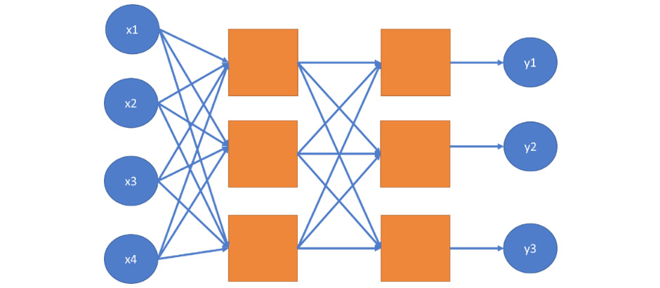
Figure 7.12: Diagram showing two hidden layers in a neural network

We can add a second layer to the equation by duplicating the weights and biases and making sure that the dimensions of the TensorFlow variables match. Note that in the first model, we transformed 784 features into 10 labels.

In this model, we will transform 784 features into a specified number of outputs. We will then take these outputs and transform them into 10 labels.

Determining the node count of the added hidden layer is not exactly science. We will use a count of 200 in this example, as it is somewhere between the feature and label dimensions.

As we have two layers, we will define two matrices (W1, W2) and vectors (b1, b2) for the weights and biases, respectively.

First, we reduce the 784 input dots using W1 and b1, and create 200 variable values. We feed these values as the input of the second layer and use W2 and b2 to create 10 label values:

x = tf.placeholder(tf.float32, [None, 28 * 28 ])

f = tf.nn.softmax

W1 = tf.Variable(tf.random_normal([784, 200]))

b1 = tf.Variable(tf.random_normal([200]))

layer1_out = f(tf.add( tf.matmul(x, W1), b1))

W2 = tf.Variable(tf.random_normal([200, 10]))

b2 = tf.Variable(tf.random_normal([10]))

y = f(tf.add(tf.matmul(layer1_out, W2), b2))

We can increase the number of layers if needed in this way. The output of layer n must be the input of layer n+1. The rest of the code remains as it is.

Convolutional Neural Networks

Convolutional Neural Networks (CNNs) are artificial neural networks that are optimized for pattern recognition. CNNs are based on convolutional layers that are among the hidden layers of the deep neural network. A convolutional layer consists of neurons that transform their inputs using a convolution operation.

When using a convolution layer, we detect patterns in the image with an m*n matrix, where m and n are less than the width and the height of the image, respectively. When performing the convolution operation, we slide this m*n matrix over the image, matching every possibility. We calculate the scalar product of the m*n convolution filter and the pixel values of the 3x3 segment of the image our convolution filter is currently on. The convolution operation creates a new image from the original one, where the important aspects of our image are highlighted, and the less-important ones are blurred.

The convolution operation summarizes information on the window it is looking at. Therefore, it is an ideal operator for recognizing shapes in an image. Shapes can be anywhere on the image, and the convolution operator recognizes similar image information regardless of its exact position and orientation. Convolutional neural networks are outside the scope of this book, because it is a more advanced topic.

Activity 15: Written Digit Detection with Deep Learning

In this section, we will discuss how deep learning improves the performance of your model. We will be assuming that your boss is not satisfied with the results you presented in Activity 14 and has asked you to consider adding two hidden layers to your original model to determine whether new layers improve the accuracy of the model. To ensure that you are able to complete this activity correctly, you will need to be knowledgeable of deep learning:

1. Execute the steps from the previous activity and measure the accuracy of the model.
2. Change the neural network by adding new layers. We will combine the ReLU and softmax activator functions.
3. Retrain the model.
4. Evaluate the model. Find the accuracy score.
5. Run the code 50 times.
6. Print the confusion matrix.

This deep neural network behaves even more chaotically than the single layer one. It took 600 iterations of 200 samples to get from an accuracy of 0.572 to 0.5723. Not long after this iteration, we jumped from 0.6076 to 0.6834 in the same number of iterations.

Due to the flexibility of the deep neural network, we expect to reach an accuracy ceiling later than in the case of the simple model. Due to the complexity of a deep neural network, it is also more likely that it gets stuck at a local maximum for a long time.

Note

The solution for this activity can be found on page 302.

Summary

In this book, we have learned about the fundamentals of AI and applications of AI in chapter on principles of AI, then we wrote a Python code to model a Tic-Tac-Toe game.

In the chapter AI with Search Techniques and Games, we solved the Tic-Tac-Toe game with game AI tools and search techniques. We learned about the search algorithms of Breadth First Search and Depth First Search. The A* algorithm helped students model a pathfinding problem. The chapter was concluded with modeling multiplayer games.

In the next couple of chapters, we learned about supervised learning using regression and classification. These chapters included data preprocessing, train-test splitting, and models that were used in several real-life scenarios. Linear regression, polynomial regression, and Support Vector Machines all came in handy when it came to predicting stock data. Classification was performed using the k-nearest neighbor and Support Vector classifiers. Several activities helped students apply the basics of classification an interesting real-life use case: credit scoring.

In Chapter 5, Using Trees for Predictive Analysis, we were introduced to decision trees, random forests, and extremely randomized trees. This chapter introduced different means to evaluating the utility of models. We learned how to calculate the accuracy, precision, recall, and F1 Score of models. We also learned how to create the confusion matrix of a model. The models of this chapter were put into practice through the evaluation of car data.

Unsupervised learning was introduced in Chapter 6, Clustering, along with the k-means and mean shift clustering algorithms. One interesting aspect of these algorithms is that the labels are not given in advance, but they are detected during the clustering process.

This book was concluded with Chapter 7, Deep Learning with Neural Networks, where neural networks and deep learning using TensorFlow was presented. We used these techniques on a real-life example: the detection of written digits.