5

Using Trees for Predictive Analysis

Learning Objectives

By the end of this chapter, you will be able to:

• Understand the metrics used for evaluating the utility of a data model
• Classify datapoints based on decision trees
• Classify datapoints based on the random forest algorithm

In this chapter, we will learn about two types of supervised learning algorithm in detail. The first algorithm will help us to classify data points using decision trees, while the other algorithm will help us classify using random forests.

Introduction to Decision Trees

In decision trees, we have input and corresponding output in the training data. A decision tree, like any tree, has leaves, branches, and nodes. Leaves are the end nodes like a yes or no. Nodes are where a decision is taken. A decision tree consists of rules that we use to formulate a decision on the prediction of a data point.

Every node of the decision tree represents a feature and every edge coming out of an internal node represents a possible value or a possible interval of values of the tree. Each leaf of the tree represents a label value of the tree.

As we learned in the previous chapters, data points have features and labels. A task of a decision tree is to predict the label value based on fixed rules. The rules come from observing patterns on the training data.

Let's consider an example of determining the label values

Suppose the following training dataset is given. Formulate rules that help you determine the label value:

Figure 5.1: Dataset to formulate the rules

In this example, we predict the label value based on four features. To set up a decision tree, we have to make observations on the available data. Based on the data that's available to us, we can conclude the following:

• All house loans are determined as credit-worthy.
• Studies loans are credit-worthy as long as the debtor is employed. If the debtor is not employed, he/she is not creditworthy.
• Loans are credit-worthy above 75,000/year income.
• At or below 75,000/year, car loans are credit-worthy whenever the debtor is not employed.

Depending on the order of how we take these rules into consideration, we can build a tree and describe one possible way of credit scoring. For instance, the following tree maps the preceding four rules:

Figure 5.2: Decision Tree for the loan type

We first determine the loan type. House loans are automatically credit-worthy according to the first rule. Studies loans are described by the second rule, resulting in a subtree containing another decision on employment. As we have covered both house and studies loans, there are only car loans left. The third rule describes an income decision, while the fourth rule describes a decision on employment.

Whenever we have to score a new debtor to determine if he/she is credit-worthy, we have to go through the decision tree from top to bottom and observe the true or false value at the bottom.

Obviously, a model based on seven data points is highly inaccurate, because we can generalize rules that simply do not match reality. Therefore, rules are often determined based on large amounts of data.

This is not the only way that we can create a decision tree. We can build decision trees based on other sequences of rules, too. Let's extract some other rules from the Dataset in Figure 5.1.

Observation 1: Notice that individual salaries that are strictly greater than 75,000 are all credit-worthy. This means that we can classify four out of seven data points with one decision.

Rule 1: Income > 75,000 => CreditWorthy is true.

Rule 1 classifies four out of seven data points; we need more rules for the remaining three data points.

Observation 2: Out of the remaining three data points, two are not employed. One is employed and is not credit worthy. With a vague generalization, we can claim the following rule:

Rule 2: Assuming Income <= 75,000, the following holds: Employed == true => CreditWorthy is false.

The first two rules classify five data points. Only two data points are left. We know that their income is less than or equal to 75,000 and that none of them are employed. There are some differences between them, though:

• The credit-worthy person makes 75,000, while the non-credit-worthy person makes 25,000.
• The credit-worthy person took a car loan, while the non-credit-worthy person took a studies loan.
• The credit-worthy person took a loan of 30,000, while the non-credit-worthy person took a loan of 15,000

Any of these differences can be extracted into a rule. For discrete ranges, such as car, studies, and house, the rule is a simple membership check. In the case of continuous ranges such as salary and loan amount, we need to determine a range to branch off.

Let's suppose that we chose the loan amount as a basis for our third rule.

Rule 3:

Assuming Income <= 75,000 and Employed == false,

If LoanAmount <= AMOUNT

Then CreditWorthy is false

Else CreditWorthy is true

The first line describes the path that leads to this decision. The second line formulates the condition, and the last two lines describe the result.

Notice that there is a constant AMOUNT in the rule. What should AMOUNT be equal to?

The answer is, any number is fine in the range 15,000 <= AMOUNT < 30,000. We are free to select any number. In this example, we chose the bottom end of the range:

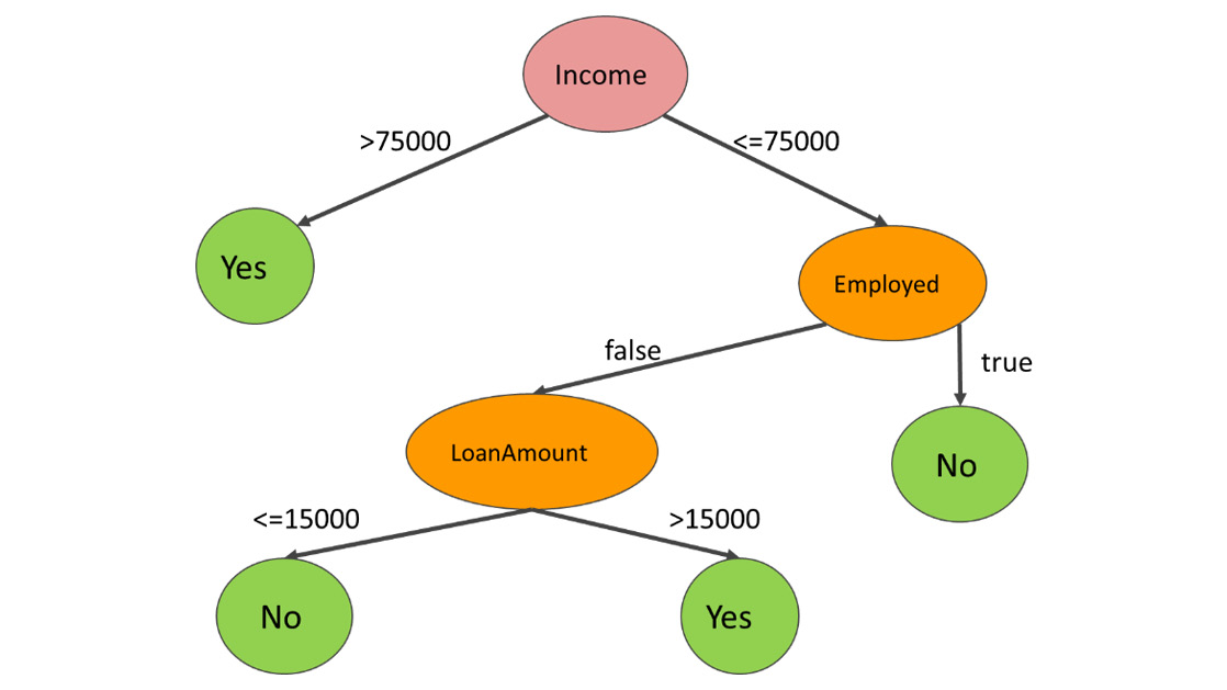
Figure 5.3: Decision Tree for Income

The second decision tree is less complex. At the same time, we cannot overlook the fact that the model says, "higher loan amounts are more likely to be repaid than lower loan amounts." It is also hard to overlook the fact that employed people with a lower income never pay back their loans. Unfortunately, there is not enough training data available, which makes it likely that we end up with false conclusions.

Overfitting is a frequent problem in decision trees when making a decision based on a few data points. This decision is rarely representative.

Since we can build decision trees in any possible order, it makes sense to define the desired way of algorithmically constructing a decision tree. Therefore, we will now explore a good measure for optimally ordering the features in the decision process.

Entropy

In information theory, entropy measures how randomly distributed the possible values of an attribute are. The higher the degree of randomness, the higher the entropy of the attribute.

Entropy is the highest possibility of an event. If we know beforehand what the outcome will be then the event has no randomness. So, entropy is zero.

When measuring the entropy of a system to be classified, we measure the entropy of the label.

Entropy is defined as follows:

• [v1, v2, ..., vn] are the possible values of an attribute
• [p1, p2, ..., pn] is the probability of these values occurring for that attribute assuming the values are equally distributed
• p1 + p2 + ... + pn = 1
  

Figure 5.4: Entropy Formula

The symbol of entropy is H in information theory. Not because entropy has anything to do with the h sound, but because H is the symbol for the upper-case Greek letter eta. Eta is, the symbol of entropy.

Note

We use entropy to order the nodes in the decision tree because the lower the entropy, the less randomly its values are distributed. The less randomness there is in the distribution, the more likely it is that the value of the label can be determined.

To calculate the entropy of a distribution in Python, we have to use the NumPy library:

import numpy as np

distribution = list(range(1,4))

minus_distribution = [-x for x in distribution]

log_distribution = [x for x in map(np.log2,distribution)]

entropy_value = np.dot(minus_distribution, log_distribution)

The distribution is given as a NumPy array or a regular list. On line 2, you have to insert your own distribution in place of [p1, p2, …, pn].

We need to create a vector of the negated values of the distribution in line 3.

On line 4, we must take the base 2 logarithm of each value in the distribution list

Finally, we calculate the sum with the scalar product, also known as the dot product of the two vectors.

Let's define the preceding calculation in the form of a function:

def entropy(distribution):

    minus_distribution = [-x for x in distribution]

    log_distribution = [x for x in map(np.log2, distribution)]

    return np.dot(minus_distribution, log_distribution)

Note

You first learned about the dot product in Chapter 3, Regression. The dot product of two vectors is calculated by multiplying the ith coordinate of the first vector by the ith coordinate of the second vector, for each i. Once we have all of the products, we sum the values:

np.dot([1, 2, 3], [4, 5, 6]) # 1*4 + 2*5 + 3*6 = 32

Exercise 15: Calculating the Entropy

Calculate the entropy of the features in the dataset in Figure 5.1.

We will calculate entropy for all features.

1. We have four features: Employed, Income, LoanType, and LoanAmount. For simplicity, we will treat the values in Income and LoanAmount as discrete values for now.
2. The following is the distribution of values for Employed:

   true 4/7 times

   false 3/7 times

3. Let's use the entropy function to calculate the entropy of the Employed column:

   H_employed = entropy([4/7, 3/7])

   The output is 0.9852.

4. The following is the distribution of values for Income:

   25,000 1/7 times

   75,000 2/7 times

   80,000 1/7 times

   100,000 2/7 times

   125,000 1/7 times

5. Let's use the entropy function to calculate the entropy of the Income column:

   H_income = entropy([1/7, 2/7, 1/7, 2/7, 1/7])

   The output is 2.2359.

6. The following is the distribution of values for LoanType:

   car 3/7 times

   studies 2/7 times

   house 2/7 times

7. Let's use the entropy function to calculate the entropy of the LoanType column:

   H_loanType = entropy([3/7, 2/7, 2/7])

   The output is 1.5567.

8. The following is the distribution of values for LoanAmount:

   15,000 1/7 times

   25,000 1/7 times

   30,000 3/7 times

   125,000 1/7 times

   150,000 1/7 times

9. Let's use the entropy function to calculate the entropy of the LoanAmount column:

   H_LoanAmount = entropy([1/7, 1/7, 3/7, 1/7, 1/7])

   The output is 2.1281.

10. As you can see, the closer the distribution is to the uniform distribution, the higher the entropy.
11. In this exercise, we were cheating a bit, because these are not the entropies that we will be using to construct the tree. In both trees, we had conditions like "greater than 75,000". We will therefore calculate the entropies belonging to the decision points we used in our original trees as well.
12. The following is the distribution of values for Income>75000

    true 4/7 times

    false 3/7 times

13. Let's use the entropy function to calculate the entropy of the Income>75,000 column:

    H_incomeMoreThan75K = entropy([4/7, 3/7])

    The output is 0.9852.

14. The following is the distribution of values for LoanAmount>15000

    true 6/7 times

    false 1/7 times

15. Let's use the entropy function to calculate the entropy of the LoanAmount

    >15,000 column:

    H_loanMoreThan15K = entropy([6/7, 1/7])

    The output is 0.5917.

Intuitively, the distribution [1] is the most deterministic distribution. This is because we know for a fact that there is 100% chance that the value of a feature stays fixed.

H([1]) = 1 * np.log2( 1 ) # 1*0 =0

We can conclude that the entropy of a distribution is strictly non-negative.

Information Gain

When we partition the data points in a dataset according to the values of an attribute, we reduce the entropy of the system.

To describe information gain, we can calculate the distribution of the labels. Initially, we have five credit-worthy and two not credit-worthy individuals in our dataset. The entropy belonging to the initial distribution is as follows:

H_label = entropy([5/7, 2/7])

0.863120568566631

Let's see what happens if we partition the dataset based on whether the loan amount is greater than 15,000 or not.

• In group 1, we get one data point belonging to the 15,000 loan amount. This data point is not credit-worthy.
• In group 2, we have 5 credit-worthy and 1 non-credit-worthy individuals.

The entropy of the labels in each group is as follows:

H_group1 = entropy([1]) #0

H_group2 = entropy([5/6, 1/6]) #0.65

To calculate the information gain, let's calculate the weighted average of the group entropies:

H_group1 * 1/7 + H_group2 * 6/7 #0.55

Information_gain = 0.8631 – 0.5572 #0.30

When creating the decision tree, on each node, our job is to partition the dataset using a rule that maximizes the information gain.

We could also use Gini Impurity instead of entropy-based information gain to construct the best rules for splitting decision trees.

Gini Impurity

Instead of entropy, there is another widely used metric that can be used to measure the randomness of a distribution: Gini Impurity.

Gini Impurity is defined as follows:

Fig 5.5: Gini Impurity

For two variables, the Gini Impurity is:

Fig 5.6: Gini Impurity for two variables

Entropy may be a bit slower to calculate because of the usage of the logarithm. Gini Impurity, on the other hand, is less precise when it comes to measuring randomness.

Note

Is information gain with entropy or Gini Impurity better for creating a decision tree?

Some people prefer Gini Impurity, because you don't have to calculate with logarithms. Computation-wise, none of the solutions are particularly complex, and so both of them can be used. When it comes to performance, the following study concluded that there are often just minimal differences between the two metrics: https://www.unine.ch/files/live/sites/imi/files/shared/documents/papers/Gini_index_fulltext.pdf.

We have learned that we can optimize a decision tree based on information gain or Gini Impurity. Unfortunately, these metrics are only available for discrete values. What if the label is defined on a continuous interval such as a price range or salary range?

We have to use other metrics. You can technically understand the idea behind creating a decision tree based on a continuous label, which was about regression. The metric we can reuse from this chapter is the mean squared error. Instead of Gini Impurity or information gain, we have to minimize the mean squared error to optimize the decision tree. As this is a beginner's book, we will omit this metric.

Exit Condition

We can continuously split the data points according to rule values until each leaf of the decision tree has an entropy of zero. The question is whether this end state is desirable.

Often, this state is not desirable, because we risk overfitting the model. When our rules for the model are too specific and too nitpicky, and the sample size on which the decision was made is too small, we risk making a false conclusion, thus recognizing a pattern in the dataset that simply does not exist in real life.

For instance, if we spin a roulette wheel three times and we get 12, 25, 12, concluding that every odd spin result in the value 12 is not a sensible strategy. By assuming that every odd spin equals 12, we find a rule that is exclusively due to random noise.

Therefore, posing a restriction on the minimum size of the dataset that we can still split is an exit condition that works well in practice. For instance, if you stop splitting as soon as you have a dataset that's lower than 50, 100, 200, or 500 in size, you avoid drawing conclusions on random noise, and so you minimize the risk of overfitting the model.

Another popular exit condition is a maximum restriction on the depth of the tree. Once we reach a fixed tree depth, we classify the data points in the leaves.

Building Decision Tree Classifiers using scikit-learn

We have already learned how to load data from a .csv file, how to apply preprocessing on the data, and how to split data into a training and testing dataset. If you need to refresh yourself on this knowledge, go back to previous chapters, where you go through this process in the context of regression and classification.

We will now assume that a set of training features, training labels, testing features, and testing labels are given as a return value of the scikit-learn train-test-split call.

Notice that, in older versions of scikit-learn, you have to import cross_validation instead of model selection:

features_train, features_test, label_train, label_test =

    model_selection.train_test_split(

        features,

        label,

        test_size=0.1

    )

We will not focus on how we got these data points, because the process is exactly the same as in the case of regression and classification.

It's time to import and use the decision tree classifier of scikit-learn:

from sklearn.tree import DecisionTreeClassifier

decision_tree = DecisionTreeClassifier(max_depth=6)

decision_tree.fit( features_train, label_train )

We set one optional parameter in the DecisionTreeClassifier, that is, max_depth, to limit the depth of the decision tree. You can read the official documentation for a full list of parameters: http://scikit-learn.org/stable/modules/generated/sklearn.tree.DecisionTreeClassifier.html. Some of the more important parameters are as follows:

• criterion: Gini stands for Gini Impurity, while entropy stands for information gain.
• max_depth: This is the maximum depth of the tree.
• min_samples_split: This is the minimum number of samples needed to split an internal node.

You can also experiment with all of the other parameters enumerated in the documentation. We will omit them in this topic.

Once the model has been built, we can use the decision tree classifier to predict data:

decision_tree.predict(features_test)

You will build a decision tree classifier in the activity at the end of this topic.

Evaluating the Performance of Classifiers

After splitting training and testing data, the decision tree model has a score method to evaluate how well testing data is classified by the model. We already learned how to use the score method in Chapters 3 and 4:

decision_tree.score(features_test, label_test)

The return value of the score method is a number that's less than or equal to 1. The closer we get to 1, the better our model is.

We will now learn another way to evaluate the model. Feel free to use this method on the models you constructed in the previous chapter as well.

Suppose we have one test feature and one test label:

# testLabel denotes the test label

predicted_label = decision_tree.predict(testFeature)

Suppose we are investigating a label value, positiveValue.

We will use the following definitions to define some metrics that help you evaluate how good your classifier is:

• Definition (True Positive): positiveValue == predictedLabel == testLabel
• Definition (True Negative): positiveValue != predictedLabel == testLabel
• Definition (False Positive): positiveValue == predictedLabel != testLabel
• Definition (False Negative): positiveValue != predictedLabel != testLabel

A false positive is a prediction that is equal to the positive value, but the actual label in the test data is not equal to this positive value. For instance, in a tech interview, a false positive is an incompetent software developer who got hired because he acted in a convincing manner, hiding his complete lack of competence.

Don't confuse a false positive with a false negative. Using the tech interview example, a false negative is a software developer who was competent enough to do the job, but he did not get hired.

Using the preceding four definitions, we can define three metrics that describe how well our model predicts reality. The symbol #( X ) denotes the number of values in X. Using technical terms, #( X ) denotes the cardinality of X:

Definition (Precision):

#( True Positives ) / (#( True Positives ) + #( False Positives ))

Definition (Recall):

#( True Positives ) / (#( True Positives ) + #( False Negatives ))

Precision centers around values that our classifier found to be positive. Some of these results are true positive, while others are false positive. A high precision means that the number of false positive results are very low compared to true positive results. This means that a precise classifier rarely makes a mistake when finding a positive result.

Recall that centers around values are positive among the test data. Some of these results are found by the classifier. These are the true positive values. Those positive values that are not found by the classifier are false negatives. A classifier with a high recall value finds most of the positive values.

Exercise 16: Precision and Recall

Find the precision and the recall value of the following two classifiers:

# Classifier 1

TestLabels1 = [True, True, False, True, True]

PredictedLabels1 = [True, False, False, False, False]

# Classifier 2

TestLabels2 = [True, True, False, True, True]

PredictedLabels = [True, True, True, True, True]

1. According to the formula let's calculate the number of true positives, false positives, and false negatives for classifier 1:

   TruePositives1 = 1 # both the predicted and test labels are true

   FalsePositives1 = 0 # predicted label is true, test label is false

   FalseNegatives1 = 3 # predicted label is false, test label is true

   Precision1 = TruePositives1 / (TruePositives1 + FalsePositives1)

   Precision1 # 1/1 = 1

   Recall1 = TruePositives1 / (TruePositives1 + FalseNegatives1)

   Recall1 #1/4 = 0.25

2. The first classifier has excellent precision, but bad recall. Let's calculate the same for the second classifier.

   TruePositives2 = 4

   FalsePositives2 = 1

   FalseNegatives2 = 0

   Precision2 = TruePositives2 / (TruePositives2 + FalsePositives2) Precision2 #4/5 = 0.8

   Recall2 = TruePositives2 / (TruePositives2 + FalseNegatives2)

   Recall2 # 4/4 = 1

3. The second classifier has excellent recall, but its precision is not perfect.
4. The F1 score is the harmonic mean of precision and recall. Its value ranges between 0 and 1. The advantage of the F1 score is that it considers both false positives and false negatives.

Exercise 17: Calculating the F1 Score

Calculate the F1 Score of the two classifiers from the previous exercise:

1. The formula for calculating the F1 Score is as follows:

   2*Precision*Recall / (Precision + Recall)

2. The first classifier has the following F1 Score:

   2 * 1 * 0.25 / (1 + 0.25) # 0.4

3. The second classifier has the following F1 Score:

   2 * 0.8 * 1 / (0.8 + 1) # 0.888888888888889

Now that we know what precision, recall, and F1 score mean, let's use a scikit-learn utility to calculate and print these values:

from sklearn.metrics import classification_report

print(

    classification_report(

        label_test,

        decision_tree.predict(features_test)

    )

)

The output will be as follows:

             precision    recall f1-score support

          0     0.97     0.97     0.97        36

          1     1.00     1.00     1.00         5

          2     1.00     0.99     1.00     127

          3     0.83     1.00     0.91         5

avg / total     0.99     0.99     0.99     173

In this example, there are four possible label values, denoted by 0, 1, 2, and 3. In each row, you get a precision, recall, and F1 score value belonging to each possible label value. You can also see in the support column how many of these label values exist in the dataset. The last row contains an aggregated precision, recall, and f1-score.

If you used label encoding to encode string labels to numbers, you may want to perform an inverse transformation to find out which row belongs to which label. In the following example, Class is the name of the label, and labelEncoders['Class'] is the label encoder belonging to the Class label:

labelEncoders['Class'].inverse_transform([0, 1, 2, 3])

array(['acc', 'good', 'unacc', 'vgood'])

If you prefer calculating the precision, recall, and F1 Score on its own, you can use individual calls. Note that in the next example, we will call each score function twice: once with average=None, and once with average='weighted'.

When the average is specified as None, we get the score value belonging to each possible label value. You can see the same values rounded in the table if you compare the results to the first four values of the corresponding column.

When the average is specified as weighted, you get the cell value belonging to the column of the score name and the avg/total row:

from sklearn.metrics import recall_score, precision_score, f1_score

label_predicted = decision_tree.predict(features_test)

Calculating the precision score with no average can be done like so:

precision_score(label_test, label_predicted, average=None)

The output is as follows:

 array([0.97222222, 1.        , 1.        , 0.83333333])

Calculating the precision score with a weighted average can be done like so:

precision_score(label_test, label_predicted, average='weighted')

The output is 0.989402697495183.

Calculating the recall score with no average can be done like so:

recall_score(label_test, label_predicted, average=None)

The output is as follows:

 array([0.97222222, 1.        , 0.99212598, 1.        ])

Calculating the recall score with a weighted average can be done like so:

recall_score(label_test, label_predicted, average='weighted')

The output is 0.9884393063583815.

Calculating the f1_score with no average can be done like so:

f1_score(label_test, label_predicted, average=None)

The output is as follows:

 array([0.97222222, 1.        , 0.99604743, 0.90909091])

Calculating the f1_score with a weighted average can be done like so:

f1_score(label_test, label_predicted, average='weighted')

The output is 0.988690625785373.

There is one more score worth investigating: the accuracy score. Suppose #( Dataset ) denotes the length of the total dataset, or in other words, the sum of true positives, true negatives, false positives, and false negatives.

Accuracy is defined as follows:

Definition (Accuracy): #( True Positives ) + #( True Negatives ) / #( Dataset )

Accuracy is a metric that's used for determining how many times the classifier gives us the correct answer. This is the first metric we used to evaluate the score of a classifier. Whenever we called the score method of a classifier model, we calculated its accuracy:

from sklearn.metrics import accuracy_score

accuracy_score(label_test, label_predicted )

The output is 0.9884393063583815.

Calculating the decision tree score can be done like so:

decisionTree.score(features_test, label_test)

The output is 0.9884393063583815.

Confusion Matrix

We will conclude this topic with one data structure that helps you evaluate the performance of a classification model: the confusion matrix.

A confusion matrix is a square matrix, where the number of rows and columns equals the number of distinct label values. In the columns of the matrix, we place each test label value. In the rows of the matrix, we place each predicted label value.

For each data point, we add one to the corresponding cells of the confusion matrix based on the predicted and actual label value.

Exercise 18: Confusion Matrix

Construct the confusion matrix of the following two distributions:

# Classifier 1

TestLabels1 = [True, True, False, True, True]

PredictedLabels1 = [True, False, False, False, False]

# Classifier 2

TestLabels2 = [True, True, False, True, True]

PredictedLabels = [True, True, True, True, True]

1. We will start with the first classifier. The columns determine the place of the test labels, while the rows determine the place of the predicted labels. The first entry is TestLabels1[0] and PredictedLabels1[0]. The values are true and true, and so we add 1 to the top-left column.
2. The second values are TestLabels1[1] = True and PredictedLabels1[1] = False. These values determine the bottom-left cell of the 2x2 matrix.
3. After finishing the placement of all five label pairs, we get the following confusion matrix:

          True False

   True     1     0

   False     3     1

4. After finishing the placement of all five label pairs, we get the following confusion matrix:

          True False

   True     4     1

   False     0     0

5. In a 2x2 matrix, we have the following distribution:

                   True            False

   True    TruePositives FalsePositives

   False FalseNegatives TrueNegatives    

6. The confusion matrix can be used to calculate precision, recall, accuracy, and f1_score metrics. The calculation is straightforward and is implied by the definitions of the metrics.
7. The confusion matrix can be calculated by scikit-learn:

   from sklearn.metrics import confusion_matrix

   confusion_matrix(label_test, label_predicted)

   array([[ 25, 0, 11, 0],

        [ 5, 0, 0, 0],

        [ 0, 0, 127, 0],

          [ 5, 0, 0, 0]])

8. Note that this is not the same example as the one we used in the previous section. Therefore, if you use the values inside the confusion matrix, you will get different precision, recall, and f1_score values.
9. You can also use pandas to create the confusion matrix:

   import pandas

   pandas.crosstab(label_test, label_predicted)

   col_0 0    2

   row_0        

   0     25 11

   1     5    0

   2     0 127

   3     5    0

Let's verify these values by calculating the accuracy score of the model:

• We have 127 + 25 = 152 data points that were classified correctly.
• The total number of data points is 152 + 11 + 5 + 5 = 173.
• 152/173 is 0.8786127167630058.

Let's calculate the accuracy score by using the scikit-learn utility we used before:

from sklearn.metrics import accuracy_score

accuracy_score(label_test, label_predicted)

The output is as follows:

0.8786127167630058

We got the same value. All of the metrics can be derived from the confusion matrix.

Activity 10: Car Data Classification

In this section, we will discuss how to build a reliable decision tree model that's capable of aiding your company in finding cars that clients are likely to buy. We will be assuming that you are employed by a car rental agency who's focusing on building a lasting relationship with its clients. Your task is to build a decision tree model that classifies cars into one of four categories: unacceptable, acceptable, good, and very good.

The dataset for this activity can be accessed here: https://archive.ics.uci.edu/ml/datasets/Car+Evaluation. Click the Data Folder link to download the dataset. Then, click the Dataset Description link to access the description of the attributes.

Let's evaluate the utility of your decision tree model:

1. Download the car data file from here: https://archive.ics.uci.edu/ml/machine-learning-databases/car/car.data. Add a header line to the front of the CSV file so that you can reference it in Python easily. We simply call the label Class. We named the six features after their descriptions in https://archive.ics.uci.edu/ml/machine-learning-databases/car/car.names.
2. Load the dataset into Python and check if it has loaded properly.

   It's time to separate the training and testing data with the cross-validation (in newer versions, this is model-selection) feature of scikit-learn. We will use 10% test data.

   Note that the train_test_split method will be available in the model_selection module, and not in the cross_validation module, starting from scikit-learn 0.20. In previous versions, model_selection already contains the train_test_split method.

   Build the decision tree classifier.

3. Check the score of our model based on the test data.
4. Create a deeper evaluation of the model based on the classification_report feature.

   Note

   The solution to this activity is available at page 282.

Random Forest Classifier

If you think about the name Random forest classifier, it makes sense to conclude the following:

• A forest consists of multiple trees.
• These trees can be used for classification.
• Since the only tree we have used so far for classification is a decision tree, it makes sense that the random forest is a forest of decision trees.
• The random nature of the trees means that our decision trees are constructed in a randomized manner.
• As a consequence, we will base our decision tree construction on information gain or Gini Impurity.

Once you understand these basic concepts, you essentially know what a Random forest classifier is all about. The more trees you have in the forest, the more accurate prediction is going to be. When performing prediction, each tree performs classification. We collect the results, and the class that gets the most votes wins.

Random forests can be used for regression as well as for classification. When using random forests for regression, instead of counting the most votes for a class, we take the average of the arithmetic mean (average) of the prediction results and return it. Random forests are not as ideal for regression as they are for classification, though, because the models used to predict values are often out of control, and often return a wide range of values. The average of these values is often not too meaningful. Managing the noise in a regression exercise is harder than in classification.

Random forests are often better than one simple decision tree because they provide redundancy. They treat outlier values better and have a lower probability of overfitting the model. Decision trees seem to behave great as long as you are using them on data that you used when creating the model. Once you use them to predict new data, random forests lose their edge. Random forests are widely used for classification problems, whether it be customer segmentation for banks or e-commerce, classifying images, or medicine. If you own an Xbox with Kinect, your Kinect device contains a random forest classifier to detect your body parts.

Random Forest Classification and regression are ensemble algorithms. The idea behind ensemble learning is that we take an aggregated view over a decision of multiple agents that potentially have different weaknesses. Due to the aggregated vote, these weaknesses cancel out, and the majority vote likely represents the correct result.

Constructing a Random Forest

One way to construct the trees of a random forest is to limit the number of features used in the classification task. Suppose you have a feature set, F. The length of the feature set is #(F). The number of features in the feature set is dim(F), where dim stands for dimension.

Suppose we limit the training data to a different subset of size s < #(F), and each random forest receives a different training data set of size s. Suppose we specify that we will use k < dim(F) features out of the possible features to construct a tree in the random forest. The selection of k features is chosen at random.

We construct each decision tree completely. Once we get a new data point to classify, we execute each tree in the random forest to perform the prediction. Once the prediction results are in, we count the votes, and the most voted class is going to be the class of the data point predicted by the random forest.

In random forest terminology, we describe the performance benefits of random forests with one word: bagging. Bagging is a technique that consists of bootstrapping and using aggregated decision making. Bootstrapping is responsible for creating a dataset that contains a subset of the entries of the original dataset. The size of the original dataset and the bootstrapped dataset is still the same because we are allowed to select the same data points multiple times in the bootstrapped dataset.

Out of bag data points are ones that don't end up in some bootstrapped datasets. To measure the out of bag error of a random forest classifier, we have to run all out of bag data points on trees of the random forest classifier that were built without considering the out of bag data points. The margin of error is the ratio between correctly classified out of bag data points and all out of bag data points.

Random Forest Classification Using scikit-learn

Our starting point is the result of the train-test splitting:

from sklearn import model_selection

features_train, features_test, label_train, label_test =

    model_selection.train_test_split(

        features,

        label,

        test_size=0.1

    )

The random forest classifier can be implemented as follows:

from sklearn.ensemble import RandomForestClassifier

random_forest_classifier = RandomForestClassifier(

    n_estimators=100,

    max_depth=6

)

randomForestClassifier.fit(features_train, label_train)

labels_predicted = random_forest_classifier.predict(features_test)

The interface of scikit-learn makes it easy to handle the random forest classifier. Throughout the last three chapters, we have already gotten used to this way of calling a classifier or a regression model for prediction.

Parameterization of the random forest classifier

As usual, consult the documentation for the full list of parameters. You can find the documentation here: http://scikit-learn.org/stable/modules/generated/sklearn.ensemble.RandomForestClassifier.html#sklearn.ensemble.RandomForestClassifier.

We will only consider a subset of the possible parameters, based on what you already know, which is based on the description of constructing random forests:

• n_estimators: The number of trees in the random forest. The default value is 10.
• criterion: Use Gini or entropy to determine whether you use Gini Impurity or information gain using entropy in each tree.
• max_features: The maximum number of features considered in any tree of the forest. Possible values include an integer. You can also add some strings such as "sqrt" for the square root of the number of features.
• max_depth: The maximum depth of each tree.
• min_samples_split: The minimum number of samples in the dataset in a given node to perform a split. This may also reduce the tree's size.
• bootstrap: A Boolean indicating whether to use bootstrapping on data points when constructing trees.

Feature Importance

A random forest classifier gives you information on how important each feature in data classification is. Remember, we use a lot of randomly constructed decision trees to classify data points. We can measure how accurately these data points behave, and we can also see which features are vital in decision making.

We can retrieve the array of feature importance scores with the following query:

random_forest_classifier.feature_importances_

The output is as follows:

array([0.12794765, 0.1022992 , 0.02165415, 0.35186759, 0.05486389,

       0.34136752])

In this six-feature classifier, the fourth and the sixth features are clearly a lot more important than any other features. The third feature has a very low importance score.

Feature importance scores come in handy when we have a lot of features and we want to reduce the feature size to avoid the classifier getting lost in the details. When we have a lot of features, we risk overfitting the model. Therefore, reducing the number of features by dropping the least significant ones is often helpful.

Extremely Randomized Trees

Extremely randomized trees increase randomization inside random forests by randomizing the splitting rules on top of the already randomized factors in random forests.

The parameterization is similar to the random forest classifier. You can see the full list of parameters here: http://scikit-learn.org/stable/modules/generated/sklearn.ensemble.ExtraTreesClassifier.html.

The Python implementation is as follows:

from sklearn.ensemble import ExtraTreesClassifier

extra_trees_classifier = ExtraTreesClassifier(

    n_estimators=100,

    max_depth=6

)

extra_trees_classifier.fit(features_train, label_train)

labels_predicted = extra_trees_classifier.predict(features_test)

Activity 11: Random Forest Classification for Your Car Rental Company

In this section, we will optimize your classifier so that you satisfy your clients more when selecting future cars for your car fleet. We will be performing random forest and Extreme random forest classification on the car dealership dataset that you worked on in previous activity of this chapter. Suggest further improvements for the model to improve the performance of the classifier:

1. Follow steps 1 to 5 of previous activity.
2. If you are using IPython, your variables may already be accessible in your console.
3. Create a random forest and an extremely randomized trees classifier and train the models.
4. Estimate how well the two models perform on the test data. We can also calculate the accuracy scores.
5. As a first optimization technique, let's see which features more important and which features are less important. Due to randomization, removing the least important features may reduce the random noise in the model.
6. Remove the third feature from the model and retrain the classifier. Compare how well the new models fare compared to the original ones.
7. Tweak the parameterization of the classifiers a bit more.

Note that we reduced the amount of nondeterminism by allowing the maximum number of features to go up to this could eventually lead to some degree of overfitting.

Note

The solution to this activity is available at page 285.

Summary

In this chapter, we have learned how to use decision trees for prediction. Using ensemble learning techniques, we created complex reinforcement learning models to predict the class of an arbitrary data point.

Decision trees on their own proved to be very accurate on the surface, but they were prone to overfitting the model. Random Forests and Extremely Randomized Trees combat overfitting by introducing some random elements and a voting algorithm, where the majority wins.

Beyond decision trees, random forests, and Extremely Randomized Trees, we also learned about new methods for evaluating the utility of a model. After using the well-known accuracy score, we started using the precision, recall, and F1 score metrics to evaluate how well our classifier works. All of these values were derived from the confusion matrix.

In the next chapter, we will describe the clustering problem and compare and contrast two clustering algorithms.