1
Learning Objectives
By the end of this chapter, you will be able to:
- Describe the various fields of AI
- Explain the main learning models used in AI
- Explain why Python is a popular language for AI projects
- Model the state space in AI for a given game
In this chapter, you will learn about the purpose, fields, and applications of AI, coupled with a short summary of the features we'll use in Python.
Introduction
Before discussing different AI techniques and algorithms, we will look at the fundamentals of artificial intelligence and machine learning and go over a few basic definitions. Then, using engaging examples, we will move forward in the book. Real-world examples will be used to present the basic concepts of artificial intelligence in an easy-to-digest way.
If you want to be an expert at something, you need to be very good at the fundamentals. So, let's begin by understanding what artificial intelligence is:
Definition: Artificial Intelligence (AI) is a science that's used to construct intelligence using hardware and software solutions.
It is inspired by reverse engineering, for example, in the way that neurons work in the human brain. Our brain consists of small units called neurons, and networks of neurons called neural networks. Beyond neural networks, there are many other models in neuroscience that can be used to solve real-world problems in artificial intelligence.
Machine learning is a term that is often confused with artificial intelligence. It originates from the 1950s, and it was first defined by Arthur Lee Samuel in 1959.
Definition: Machine learning is a field of study concerned with giving computers the ability to learn without being explicitly programmed.
Tom Mitchell proposed a more mathematically precise definition of machine learning.
Definition: A computer program is said to learn from experience, E, with respect to a task, T, and a performance measure, P, if its performance on T, as measured by P, improves with experience E.
From these two definitions, we can conclude that machine learning is one way to achieve artificial intelligence. However, you can have artificial intelligence without machine learning. For instance, if you hardcode rules and decision trees, or you apply search techniques, you create an artificial intelligence agent, even though your approach has little to do with machine learning.
How does AI Solve Real World Problems?
Artificial intelligence automates human intelligence based on the way human brain processes information.
Whenever we solve a problem or interact with people, we go through a process. Whenever we limit the scope of a problem or interaction, this process can often be modeled and automated.
AI makes computers appear to think like humans.
Sometimes, it feels like AI knows what we need. Just think about the personalized coupons you receive after shopping online. By the end of this book, you will understand that to choose the most successful products, you need to be shown how to maximize your purchases – this is a relatively simple task. However, it is also so efficient, that we often think that computers "know" what we need.
AI is performed by computers that are executing low-level instructions.
Even though a solution may appear to be intelligent, we write code, just like with any other software solutions. Even if we are simulating neurons, simple machine code and computer hardware executes the "thinking" process.
Most AI applications have one primary objective. When we interact with an AI application, it seems human-like because it can restrict a problem domain to a primary objective. Therefore, we get a chance to break down complex processes and simulate intelligence with the help of low-level computer instructions.
AI may stimulate human senses and thinking processes for specialized fields.
We must simulate human senses and thoughts, and sometimes trick AI into believing that we are interacting with another human. In special cases, we can even enhance our own senses.
Similarly, when we interact with a chatbot, we expect the bot to understand us. We expect the chatbot or even a voice recognition system to provide a computer-human interface that fulfills our expectations. In order to meet these expectations, computers need to emulate the human thought processes.
Diversity of Disciplines
A self-driving car that couldn't sense that other cars were driving on the same highway would be incredibly dangerous. The AI agent needs to process and sense what is around it in order to drive the car. But that is itself is not enough. Without understanding the physics of moving objects, driving the car in a normal environment would be an almost impossible, not to mention deadly, task.
In order to create a usable AI solution, different disciplines are involved. For example:
- Robotics: To move objects in space
- Algorithm Theory: To construct efficient algorithms
- Statistics: To derive useful results, predict the future, and analyze the past
- Psychology: To model how the human brain works
- Software Engineering: To create maintainable solutions that endure the test of time
- Computer Science or Computer Programming: To implement our software solutions in practice
- Mathematics: To perform complex mathematical operations
- Control Theory: To create feed-forward and feedback systems
- Information Theory: To represent, encode, decode, and compress information
- Graph Theory: To model and optimize different points in space and to represent hierarchies
- Physics: To model the real world
- Computer Graphics and Image Processing to display and process images and movies
In this book, we will cover a few of these disciplines. Remember, focus is power, and we are now focusing on a high-level understanding of artificial intelligence.
Fields and Applications of Artificial Intelligence
Now that we know what Artificial Intelligence is, let's move on and investigate different fields in which AI is applied.
Simulation of Human Behavior
Humans have five basic senses simply divided into visual, auditory, kinesthetic, olfactory, and gustatory. However, for the purposes of understanding how to create intelligent machines, we can separate disciplines as follows:
- Listening and speaking
- Understanding language
- Remembering things
- Thinking
- Seeing
- Moving
A few of these are out of scope for us, because the purpose of this book is to understand the fundamentals. In order to move a robot arm, for instance, we would have to study complex university-level math to understand what's going on.
Listening and Speaking
Using speech recognition system, AI can collect the information. Using speech synthesis, it can turn internal data into understandable sounds. Speech recognition and speech synthesis techniques deal with the recognition and construction of sounds humans emit or that humans can understand.
Imagine you are on a trip to a country where you don't speak the local language. You can speak into the microphone of your phone, expect it to "understand" what you say, and then translate it into the other language. The same can happen in reverse with the locals speaking and AI translating the sounds into a language you understand. Speech recognition and speech synthesis make this possible.
Note
An example of speech synthesis is Google Translate. You can navigate to https://translate.google.com/ and make the translator speak words in a non-English language by clicking the loudspeaker button below the translated word.
Understanding Language
We can understand natural language by processing it. This field is called natural language processing, or NLP for short.
When it comes to natural language processing, we tend to learn languages based on statistical learning.
Remembering Things
We need to represent things we know about the world. This is where creating knowledge bases and hierarchical representations called ontologies comes into play. Ontologies categorize things and ideas in our world and contain relations between these categories.
Thinking
Our AI system has to be an expert in a certain domain by using an expert system. An expert system can be based on mathematical logic in a deterministic way, as well as in a fuzzy, non-deterministic way.
The knowledge base of an expert system is represented using different techniques. As the problem domain grows, we create hierarchical ontologies.
We can replicate this structure by modeling the network on the building blocks of the brain. These building blocks are called neurons, and the network itself is called a neural network.
There is another key term you need to connect to neural networks: deep learning. Deep learning is deep because it goes beyond pattern recognition and categorization. Learning is imprinted into the neural structure of the network. One special deep learning task, for instance, is object recognition using computer vision.
Seeing
We have to interact with the real world through our senses. We have only touched upon auditory senses so far, in regard to speech recognition and synthesis. What if we had to see things? Then, we would have to create computer vision techniques to learn about our environment. After all, recognizing faces is useful, and most humans are experts at that.
Computer vision depends on image processing. Although image processing is not directly an AI discipline, it is a required discipline for AI.
Moving
Moving and touching are natural to us humans, but they are very complex tasks for computers. Moving is handled by robotics. This is a very math-heavy topic.
Robotics is based on control theory, where you create a feedback loop and control the movement of your object based on the feedback gathered. Interestingly enough, control theory has applications in other fields that have absolutely nothing to do with moving objects in space. This is because the feedback loops required are similar to those modeled in economics.
Simulating Intelligence – The Turing Test
Alan Turing, the inventor of the Turing machine, an abstract concept that's used in algorithm theory, suggested a way to test intelligence. This test is referred to as the Turing test in AI literature.
Using a text interface, an interrogator chats to a human and a chatbot. The job of the chatbot is to mislead the interrogator to the extent that they cannot tell whether the computer is human or not.
What disciplines do we need to pass the Turing test?
First of all, we need to understand a spoken language to know what the interrogator is saying. We do this by using Natural Language Processing (NLP). We also have to respond.
We need to be an expert on things that the human mind tends to be interested in. We need to build an Expert System of humanity, involving the taxonomy of objects and abstract thoughts in our world, as well as historical events and even emotions.
Passing the Turing test is very hard. Current predictions suggest we won't be able to create a system good enough to pass the Turing test until the late 2020's. Pushing this even further, if this is not enough, we can advance to the Total Turing Test, which also includes movement and vision.
AI Tools and Learning Models
In the previous sections, we discovered the fundamentals of artificial intelligence. One of the core tasks for artificial intelligence is learning.
Intelligent Agents
When solving AI problems, we create an actor in the environment that can gather data from its surroundings and influence its surroundings. This actor is called an intelligent agent.
An intelligent agent:
- Is autonomous
- Observes its surroundings through sensors
- Acts in its environment using actuators
- Directs its activities toward achieving goals
Agents may also learn and have access to a knowledge base.
We can think of an agent as a function that maps perceptions to actions. If the agent has an internal knowledge base, perceptions, actions, and reactions may alter the knowledge base as well.
Actions may be rewarded or punished. Setting up a correct goal and implementing a carrot and stick situation helps the agent learn. If goals are set up correctly, agents have a chance of beating the often more complex human brain. This is because the number one goal of the human brain is survival, regardless of the game we are playing. An agent's number one motive is reaching the goal itself. Therefore, intelligent agents do not get embarrassed when making a random move without any knowledge.
Classification and Prediction
Different goals require different processes. Let's explore the two most popular types of AI reasoning: classification and prediction.
Classification is a process for figuring out how an object can be defined in terms of another object. For instance, a father is a male who has one or more children. If Jane is a parent of a child and Jane is female, then Jane is a mother. Also, Jane is a human, a mammal, and a living organism. We know that Jane has a nationality as well as a date of birth.
Prediction is the process of predicting things, based on patterns and probabilities. For instance, if a customer in a standard supermarket buys organic milk, the same customer is more likely to buy organic yoghurt than the average customer.
Learning Models
The process of AI learning can be done in a supervised or unsupervised way. Supervised learning is based on labeled data and inferring functions from training data. Linear regression is one example. Unsupervised learning is based on unlabeled data and often works on cluster analysis.
The Role of Python in Artificial Intelligence
In order to put the basic AI concepts into practice, we need a programming language that supports artificial intelligence. In this book, we have chosen Python. There are a few reasons why Python is such a good choice for AI:
- Python is a high-level programming language. This means that you don't have to worry about memory allocation, pointers, or machine code in general. You can write code in a convenient fashion and rely on Python's robustness. Python is also cross-platform compatible.
- The strong emphasis on developer experience makes Python a very popular choice among software developers. In fact, according to a 2018 developer survey by https://www.hackerrank.com, across all ages, Python ranks as the number one preferred language of software developers. This is because Python is easily readable and simple. Therefore, Python is great for rapid application development.
- Despite being an interpreted language, Python is comparable to other languages used in data science such as R. Its main advantage is memory efficiency, as Python can handle large, in-memory databases.
Note
Python is a multi-purpose language. It can be used to create desktop applications, database applications, mobile applications, as well as games. The network programming features of Python are also worth mentioning. Furthermore, Python is an excellent prototyping tool.
Why is Python Dominant in Machine Learning, Data Science, and AI?
To understand the dominant nature of Python in machine learning, data science, and AI, we have to compare Python to other languages also used in these fields.
One of the main alternatives is R. The advantage of Python compared to R is that Python is more general purpose and more practical.
Compared to Java and C++, writing programs in Python is significantly faster. Python also provides a high degree of flexibility.
There are some languages that are similar in nature when it comes to flexibility and convenience: Ruby and JavaScript. Python has an advantage over these languages because of the AI ecosystem available for Python. In any field, open source, third-party library support vastly determines the success of that language. Python's third-party AI library support is excellent.
Anaconda in Python
We already installed Anaconda in the preface. Anaconda will be our number one tool when it comes to experimenting with artificial intelligence.
This list is by far incomplete, as there are more than 700 libraries available in Anaconda. However, if you know these libraries, then you're off to a good start because you will be able to implement fundamental AI algorithms in Python.
Anaconda comes with packages, IDEs, data visualization libraries, and high-performance tools for parallel computing in one place. Anaconda hides configuration problems and the complexity of maintaining a stack for data science, machine learning, and artificial intelligence. This feature is especially useful in Windows, where version mismatches and configuration problems tend to arise the most.
Anaconda comes with the IPython console, where you can write code and comments in documentation style. When you experiment with AI features, the flow of your ideas resembles an interactive tutorial where you run each step of your code.
Note
IDE stands for Integrated Development Environment. While a text editor provides some functionalities to highlight and format code, an IDE goes beyond the features of text editors by providing tools to automatically refactor, test, debug, package, run, and deploy code.
Python Libraries for Artificial Intelligence
The list of libraries presented here is not complete as there are more than 700 available in Anaconda. However, these specific ones will get you off to a good start, because they will give you a good foundation to be able to implement fundamental AI algorithms in Python:
- NumPy: NumPy is a computing library for Python. As Python does not come with a built-in array data structure, we have to use a library to model vectors and matrices efficiently. In data science, we need these data structures to perform simple mathematical operations. We will extensively use NumPy in future modules.
- SciPy: SciPy is an advanced library containing algorithms that are used for data science. It is a great complementary library to NumPy, because it gives you all the advanced algorithms you need, whether it be a linear algebra algorithm, image processing tool, or a matrix operation.
- pandas: pandas provides fast, flexible, and expressive data structures such as one-dimensional series and two-dimensional DataFrames. It efficiently loads, formats, and handles complex tables of different types.
- scikit-learn: scikit-learn is Python's main machine learning library. It is based on the NumPy and SciPy libraries. scikit-learn provides you with the functionality required to perform both classification and regression, data preprocessing, as well as supervised and unsupervised learning.
- NLTK: We will not deal with natural language processing in this book but NLTK is still worth mentioning, because this library is the main natural language toolkit of Python. You can perform classification, tokenization, stemming, tagging, parsing, semantic reasoning, and many other services using this library.
- TensorFlow: TensorFlow is Google's neural network library, and it is perfect for implementing deep learning artificial intelligence. The flexible core of TensorFlow can be used to solve a vast variety of numerical computation problems. Some real-world applications of TensorFlow include Google voice recognition and object identification.
A Brief Introduction to the NumPy Library
The NumPy library will play a major role in this book, so it is worth exploring it further.
After launching your IPython console, you can simply import NumPy as follows:
import numpy as np
Once NumPy has been imported, you can access it using its alias, np. NumPy contains the efficient implementation of some data structures such as vectors and matrices. Python does not come with a built-in array structure, so NumPy's array comes in handy. Let's see how we can define vectors and matrices:
np.array([1,3,5,7])
The output is as follows:
array([1, 3, 5, 7])
We can declare a matrix using the following syntax:
A = np.mat([[1,2],[3,3]])
A
The output is as follows:
matrix([[1, 2],
[3, 3]])
The array method creates an array data structure, while mat creates a matrix.
We can perform many operations with matrices. These include addition, subtraction, and multiplication:
Addition in matrices:
A + A
The output is as follows:
matrix([[2, 4],
[6, 6]])
Subtraction in matrices:
A - A
The output is as follows:
matrix([[0, 0],
[0, 0]])
Multiplication in matrices:
A * A
The output is as follows:
matrix([[ 7, 8],
[12, 15]])
Matrix addition and subtraction works cell by cell.
Matrix multiplication works according to linear algebra rules. To calculate matrix multiplication manually, you have to align the two matrices, as follows:

Figure 1.1: Multiplication calculation with two matrices
To get the (i,j)th element of the matrix, you compute the dot (scalar) product on the ith row of the matrix with the jth column. The scalar product of two vectors is the sum of the product of their corresponding coordinates.
Another frequent matrix operation is the determinant of the matrix. The determinant is a number associated with square matrices. Calculating the determinant using NumPy is easy:
np.linalg.det( A )
The output is -3.0000000000000004.
Technically, the determinant can be calculated as 1*3 – 2*3 = -3. Notice that NumPy calculates the determinant using floating-point arithmetic, and therefore, the accuracy of the result is not perfect. The error is due to the way floating-points are represented in most programming languages.
We can also transpose a matrix, like so:
np.matrix.transpose(A)
The output is as follows:
matrix([[1, 3],
[2, 3]])
When calculating the transpose of a matrix, we flip its values over its main diagonal.
NumPy has many other important features, and therefore, we will use it in most of the chapters in this book.
Exercise 1: Matrix Operations Using NumPy
We will be using IPython and the following matrix to solve this exercise. We will start by understanding the NumPy syntax:

Figure 1.2: Simple Matrix
Using NumPy, calculate the following:
- The square of the matrix
- The determinant of the matrix
- The transpose of the matrix
Let's begin with NumPy matrix operations:
- Import the NumPy library.
import numpy as np
- Create a two-dimensional array storing the matrix:
A = np.mat([[1,2,3],[4,5,6],[7,8,9]])
Notice the np.mat construct. If you have created an np.array instead of np.mat, the solution for the array multiplication will be incorrect.
- NumPy supports matrix multiplication by using the asterisk:
A * A
The output is as follows:
matrix([[ 30, 36, 42],
[ 66, 81, 96],
[102, 126, 150]])
As you can see from the following code, the square of A has been calculated by performing matrix multiplication. For instance, the top-left element of the matrix is calculated as follows:
1 * 1 + 2 * 4 + 3 * 7
The output is 30.
- Use np.linalg.det to calculate the determinant of the matrix:
np.linalg.det( A )
The output is -9.51619735392994e-16.
The determinant is almost zero according to the preceding calculations. This inefficiency is due to floating-point arithmetic. The actual determinant is zero.
You can conclude this by calculating the determinant manually:
1*5*9 + 2*6*7 + 3*4*8 - 1*6*8 - 2*4*9 - 3*5*7
The output is 0.
Whenever you work with NumPy, make sure that you factor in the possibility of floating-point arithmetic rounding errors, even if you appear to be working with integers.
- Use np.matrix.transpose to get the transpose of the matrix:
np.matrix.transpose(A)
The output is as follows:
matrix([[1, 4, 7],
[2, 5, 8],
[3, 6, 9]])
If T is the transpose of matrix A, then T[j][i] is equal to A[i][j].
NumPy comes with many useful features for vectors, matrices, and other mathematical structures.
Python for Game AI
An AI game player is nothing but an intelligent agent with a clear goal: to win the game and defeat all other players. Artificial Intelligence experiments have achieved surprising results when it comes to games. Today, no human can defeat an AI in the game of chess.
The game Go was the last game where human grandmasters could consistently defeat a computer player. However, in 2017, Google's game-playing AI defeated the Go grandmaster.
Intelligent Agents in Games
An intelligent agent plays according to the rules of the game. The agent can sense the current state of the game through its sensors and can evaluate the utility of potential steps. Once the agent finds the best possible step, it performs the action using its actuators. The agent finds the best possible action to reach the goal based on the information it has. Actions are either rewarded or punished. The carrot and stick are excellent examples of rewards and punishment. Imagine a donkey in front of your cart. You put a carrot in front of the eyes of the donkey, so the poor animal starts walking toward it. As soon as the donkey stops, the rider may apply punishment with a stick. This is not a human way of moving, but rewards and punishment control living organisms to some extent. The same happens to humans at school, at work, and in everyday life as well. Instead of carrots and sticks, we have income and legal punishment to shape our behavior.
In most games and gamified applications, a good sequence of actions results in a reward. When a human player feels rewarded, a hormone called dopamine is released. Dopamine is also referred to as the chemical of reward. When a human achieves a goal or completes a task, dopamine is released. This hormone makes you feel happy. Humans tend to act in a way that maximizes their happiness. This sequence of actions is called a compulsion loop. Intelligent agents, on the other hand, are only interested in their goal, which is to maximize their reward and minimize their punishment.
When modeling games, we must determine their state space. An action causes a state transition. When we explore the consequences of all possible actions, we get a decision tree. This tree goes deeper as we start exploring the possible future actions of all players until the game ends.
The strength of AI is the execution of millions of possible steps each second. Therefore, game AI often boils down to a search exercise. When exploring all of the possible sequences of moves in a game, we get the state tree of a game.
Consider a chess AI. What is the problem with evaluating all possible moves by building a state tree consisting of all of the possible sequences of moves?
Chess is an EXPTIME game complexity-wise. The number of possible moves explodes combinatorially.
White starts with 20 possible moves: the 8 pawns may move either one or two steps, and the two knights may move either up-up-left, or up-up-right. Then, black can make any of these twenty moves. There are already 20*20 = 400 possible combinations after just one move per player.
After the second move, we get 8,902 possible board constellations, and this number just keeps on growing. Just take seven moves, and you have to search through 10,921,506 possible constellations.
The average length of a chess game is approximately 40 moves. Some exceptional games take more than 200 moves to finish.
As a consequence, the computer player simply does not have time to explore the whole state space. Therefore, the search activity has to be guided with proper rewards, punishment, and simplifications of the rules.
Breadth First Search and Depth First Search
Creating a game AI is often a search exercise. Therefore, we need to be familiar with the two primary search techniques: Breadth First Search (BFS) and Depth First Search (DFS).
These search techniques are applied on a directed rooted tree. A tree is a data structure that has nodes, and edges connecting these nodes in such a way that any two nodes of the tree are connected by exactly one path:
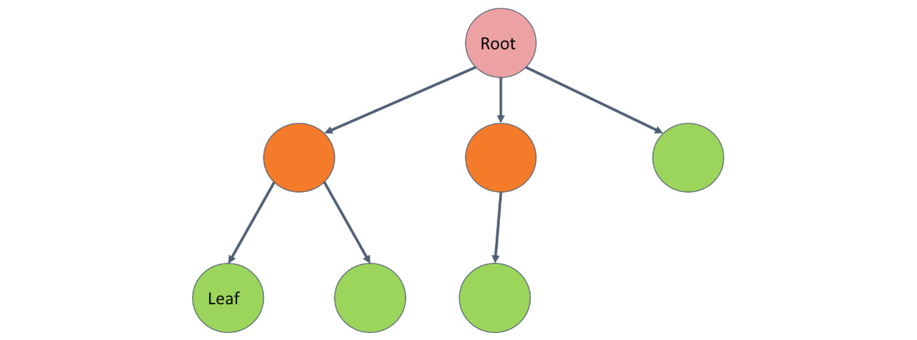
Figure 1.3: A directed rooted tree
When the tree is rooted, there is a special node in the tree called the root, where we begin our traversal. A directed tree is a tree where the edges may only be traversed in one direction. Nodes may be internal nodes or leaves. Internal nodes have at least one edge through which we can leave the node. A leaf has no edges pointing out from the node.
In AI search, the root of the tree is the starting state. We traverse from this state by generating successor nodes of the search tree. Search techniques differ regarding which order we visit these successor nodes in.
Suppose we have a tree defined by its root, and a function that generates all the successor nodes from the root. In this example, each node has a value and a depth. We start from 1 and may either increase the value by 1 or 2. Our goal is to reach the value 5.
root = {'value': 1, 'depth': 1}
def succ(node):
if node['value'] == 5:
return []
elif node['value'] == 4:
return [{'value': 5,'depth': node['depth']+1}]
else:
return [
{'value': node['value']+1, 'depth':node['depth']+1},
{'value': node['value']+2, 'depth':node['depth']+1}
]
We will first perform DFS on this example:
def bfs_tree(node):
nodes_to_visit = [node]
visited_nodes = []
while len(nodes_to_visit) > 0:
current_node = nodes_to_visit.pop(0)
visited_bodes.append(current_node)
nodes_to_visit.extend(succ(current_node))
return visited_nodes
bfs_tree(root)
The output is as follows:
[{'depth': 1, 'value': 1},
{'depth': 2, 'value': 2},
{'depth': 2, 'value': 3},
{'depth': 3, 'value': 3},
{'depth': 3, 'value': 4},
{'depth': 3, 'value': 4},
{'depth': 3, 'value': 5},
{'depth': 4, 'value': 4},
{'depth': 4, 'value': 5},
{'depth': 4, 'value': 5},
{'depth': 4, 'value': 5},
{'depth': 5, 'value': 5}]
Notice that breadth first search finds the shortest path to a leaf first, because it enumerates all nodes in the order of increasing depth.
If we had to traverse a graph instead of a directed rooted tree, breadth first search would look different: whenever we visit a node, we would have to check whether the node had been visited before. If the node had been visited before, we would simply ignore it.
In this chapter, we only use Breadth First Traversal on trees. Depth First Search is surprisingly similar to Breadth First Search. The difference between Depth First Traversals and BFS is the sequence in which you access the nodes. While BFS visits all the children of a node before visiting any other nodes, DFS digs deep in the tree first:
def dfs_tree(node):
nodes_to_visit = [node]
visited_nodes = []
while len(nodes_to_visit) > 0:
current_node = nodes_to_visit.pop()
visited_nodes.append(current_node)
nodes_to_visit.extend(succ(current_node))
return visited_nodes
dfs_tree(root)
The output is as follows:
[{'depth': 1, 'value': 1},
{'depth': 2, 'value': 3},
{'depth': 3, 'value': 5},
{'depth': 3, 'value': 4},
{'depth': 4, 'value': 5},
{'depth': 2, 'value': 2},
{'depth': 3, 'value': 4},
{'depth': 4, 'value': 5},
{'depth': 3, 'value': 3},
{'depth': 4, 'value': 5},
{'depth': 4, 'value': 4},
{'depth': 5, 'value': 5}]
As you can see, the DFS algorithm digs deep fast. It does not necessarily find the shortest path first, but it is guaranteed to find a leaf before exploring a second path.
In game AI, the BFS algorithm is often better for the evaluation of game states, because DFS may get lost. Imagine starting a chess game, where a DFS algorithm may easily get lost in searching.
Exploring the State Space of a Game
Let's explore the state space of a simple game: Tic-Tac-Toe.
In Tic-Tac-Toe, a 3x3 game board is given. Two players play this game. One plays with the sign X, and the other plays with the sign O. X starts the game, and each player makes a move after the other. The goal of the game is to get three of your own signs horizontally, vertically, or diagonally.
Let's denote the cells of the Tic-Tac-Toe board as follows:

Figure 1.4: Tic-Tac-Toe Board
In the following example, X started at position 1. O retaliated at position 5, X made a move at position 9, and then O moved to position 3:

Figure 1.5: Tic-Tac-Toe Board with noughts and crosses
This was a mistake by the second player, because now X is forced to place a sign on cell 7, creating two future scenarios for winning the game. It does not matter whether O defends by moving to cell 4 or 8 – X will win the game by selecting the other unoccupied cell.
Note
You can try out the game at http://www.half-real.net/tictactoe/.
For simplicity, we will only explore the state space belonging to the cases when the AI player starts. We will start with an AI player that plays randomly, placing a sign in an empty cell. After playing with this AI player, we will create a complete decision tree. Once we generate all possible game states, you will experience their combinatoric explosion. As our goal is to make these complexities simple, we will use several different techniques to make the AI player smarter, and to reduce the size of the decision tree. By the end of this experiment, we will have a decision tree that has less than 200 different game endings, and as a bonus, the AI player will never lose a single game.
To make a random move, you will have to know how to choose a random element from a list using Python. We will use the choice function of the random library:
from random import choice
choice([2, 4, 6, 8])
The output is 6.
The output of the choice function is a random element of the list.
Note
We will use the factorial notation in the following exercise. Factorial is denoted by the "!" exclamation mark. By definition, 0! = 1, and n! = n*(n-1)!. In our example, 9! = 9* 8! = 9*8*7! = … = 9*8*7*6*5*4*3*2*1.
Exercise 2: Estimating the Number of Possible States in Tic-Tac-Toe Game
Make a rough estimate of the number of possible states on each level of the state space of the Tic-Tac-Toe game:
- In our estimation, we will not stop until all of the cells of the board have been filled. A player might win before the game ends, but for the sake of uniformity, we will continue the game.
- The first player will choose one of the nine cells. The second player will choose one out of the eight remaining cells. The first player can then choose one out of the seven remaining cells. This goes on until either player wins the game, or the first player is forced to make the ninth and last move.
- The number of possible decision sequences are therefore 9! = 362880. A few of these sequences are invalid, because a player may win the game in less than nine moves. It takes at least five moves to win a game, because the first player needs to move three times.
- To calculate the exact size of the state space, we would have to calculate the number of games that are won in five, six, seven, and eight steps. This calculation is simple, but due to its exhaustive nature, it is out of scope for us. We will therefore settle for the magnitude of the state space.
Note
After generating all possible Tic-Tac-Toe games, researchers counted 255,168 possible games. Out of those games, 131,184 were won by the first player, 77,904 were won by the second player, and 46,080 games ended with a draw. Visit http://www.half-real.net/tictactoe/allgamesoftictactoe.zip to download all possible Tic-Tac-Toe games.
Even a simple game like Tic-Tac-Toe has a lot of states. Just imagine how hard it would be to start exploring all possible chess games. Therefore, we can conclude that brute-force search is rarely ideal.
Exercise 3: Creating an AI Randomly
In this section, we'll create a framework for the Tic-Tac-Toe game for experimentation. We will be modelling the game on the assumption that the AI player always starts the game. Create a function that prints your internal representation and allow your opponent to enter a move randomly. Determine whether a player has won. To ensure that this happens correctly, you will need to have completed the previous exercises:
- We will import the choice function from the random library:
from random import choice
- We will model the nine cells in a simple string for simplicity. A nine-character long Python string stores these cells in the following order: "123456789". Let's determine the index triples that must contain matching signs so that a player wins the game:
combo_indices = [
[0, 1, 2],
[3, 4, 5],
[6, 7, 8],
[0, 3, 6],
[1, 4, 7],
[2, 5, 8],
[0, 4, 8],
[2, 4, 6]
]
- Let's define the sign constants for empty cells, the AI, and the opponent player:
EMPTY_SIGN = '.'
AI_SIGN = 'X'
OPPONENT_SIGN = 'O'
- Let's create a function that prints a board. We will add an empty row before and after the board so that we can easily read the game state:
def print_board(board):
print(" ")
print(' '.join(board[:3]))
print(' '.join(board[3:6]))
print(' '.join(board[6:]))
print(" ")
- We will describe a move of the human player. The input arguments are the boards, the row numbers from 1 to 3, and the column numbers from 1 to 3. The return value of this function is a board containing the new move:
def opponent_move(board, row, column):
index = 3 * (row - 1) + (column - 1)
if board[index] == EMPTY_SIGN:
return board[:index] + OPPONENT_SIGN + board[index+1:]
return board
- It is time to define a random move of the AI player. We will generate all possible moves with the all_moves_from_board function, and then we will select a random move from the list of possible moves:
def all_moves_from_board_list(board, sign):
move_list = []
for i, v in enumerate(board):
if v == EMPTY_SIGN:
move_list.append(board[:i] + sign + board[i+1:])
return move_list
def ai_move(board):
return choice(all_moves_from_board(board, AI_SIGN))
- After defining the moves, we have to determine whether a player has won the game:
def game_won_by(board):
for index in combo_indices:
if board[index[0]] == board[index[1]] == board[index[2]] != EMPTY_SIGN:
return board[index[0]]
return EMPTY_SIGN
- Last, but not least, we will create a game loop so that we can test the interaction between the computer player and the human player. Although we will carry out an exhaustive search in the following examples:
def game_loop():
board = EMPTY_SIGN * 9
empty_cell_count = 9
is_game_ended = False
while empty_cell_count > 0 and not is_game_ended:
if empty_cell_count % 2 == 1:
board = ai_move(board)
else:
row = int(input('Enter row: '))
col = int(input('Enter column: '))
board = opponent_move(board, row, col)
print_board(board)
is_game_ended = game_won_by(board) != EMPTY_SIGN
empty_cell_count = sum(
1 for cell in board if cell == EMPTY_SIGN
)
print('Game has been ended.')
- Use the game_loop function to run the game:
game_loop()
As you can see, even an opponent who's playing randomly may win from time to time if their opponent makes a mistake.
Activity 1: Generating All Possible Sequences of Steps in a Tic-Tac-Toe Game
This activity will explore the combinatoric explosion that is possible when two players play randomly. We will be using a program, building on the previous results, that generates all possible sequences of moves between a computer player and a human player. Assume that the human player may make any possible move. In this example, given that the computer player is playing randomly, we will examine the wins, losses, and draws belonging to two randomly playing players:
- Create a function that maps the all_moves_from_board function on each element of a list of board spaces/squares. This way, we will have all of the nodes of a decision tree.
- The decision tree starts with [ EMPTY_SIGN * 9 ], and expands after each move. Let's create a filter_wins function that takes finished games out of the list of moves and appends them in an array containing the board states won by the AI player and the opponent player:
- Then, with a count_possibilities function that prints the number of decision tree leaves that ended with a draw, were won by the first player, and were won by the second player.
- We have up to 9 steps in each state. In the 0th, 2nd, 4th, 6th, and 8th iteration, the AI player moves. In all other iterations, the opponent moves. We create all possible moves in all steps and take out finished games from the move list.
- Then, execute the number of possibilities to experience the combinatoric explosion.
As you can see, the tree of board states consists of 266,073 leaves. The count_possibilities function essentially implements a BFS algorithm to traverse all the possible states of the game. Notice that we count these states multiple times because placing an X in the top-right corner on step 1 and placing an X in the top-left corner on step 3 leads to similar possible states as starting with the top-left corner and then placing an X in the top-right corner. If we implemented the detection of duplicate states, we would have to check fewer nodes. However, at this stage, due to the limited depth of the game, we'll omit this step.
A decision tree is very similar to the data structure examined by count_possibilities. In a decision tree, we explore the utility of each move by investigating all possible future steps up to a certain extent. In our example, we could calculate the utility of the first moves by observing the number of wins and losses after fixing the first few moves.
Note
The root of the tree is the initial state. An internal state of the tree is a state in which a game has not been ended and moves are possible. A leaf of the tree contains a state where a game has ended.
The solution for this activity can be found on page 258.
Summary
In this chapter, we have learned what Artificial Intelligence is, as well as its multiple disciplines.
We have seen how AI can be used to enhance or substitute human brainpower, to listen, speak, understand language, store and retrieve information, think, see, and move. Then, we moved on to learn about intelligent agents that act in their environment, solving a problem in a seemingly intelligent way to pursue a previously determined goal. When agents learn, they can learn in a supervised or an unsupervised way. We can use intelligent agents to classify things or make predictions about the future.
We then introduced Python and learned about its role in the field of Artificial Intelligence. We looked at a few important Python libraries for developing intelligent agents and preparing data for agents. As a warm-up, we concluded this chapter with an example, where we used the NumPy library to perform some matrix operations in Python. We also learned how to create a search space for a Tic Tac Toe game. In the next chapter, we will learn how intelligence can be imparted with the help of search space.