
2
Learning Objectives
By the end of this chapter, you will be able to:
- Build a simple game AI with Python based on static rules
- Determine the role of heuristics in Game AI
- Employ search techniques and pathfinding algorithms
- Implement game AI for two-player games with the Minmax algorithm
In this chapter, we will be looking at creating intelligent agents.
Introduction
In the previous chapter, we understood the significance of an intelligent agent. We also examined the game states for a game AI. In this chapter, we will focus on how to create and introduce intelligence into an agent.
We will look at reducing the number of states in the state space and analyze the stages that a game board can undergo and make the environment work in such a way that we win. By the end of this chapter, we will have a Tic-Tac-Toe player who never loses a match.
Exercise 4: Teaching the Agent to Win
In this exercise, we will see how the steps needed to win can be reduced. We will be making the agent that we developed in the previous chapter detect situations where it can win a game. Compare the number of possible states to the random play as an example.
- We will be defining two functions, ai_move and all_moves_from_board. We will create ai_move so that it returns a move that will consider its own previous moves. If the game can be won in that move, ai_move will select that move.
def ai_move(board):
new_boards = all_moves_from_board(board, AI_SIGN)
for new_board in new_boards:
if game_won_by(new_board) == AI_SIGN:
return new_board
return choice(new_boards)
- Let's test the application with a game loop. Whenever the AI has the opportunity to win the game, it will always place the X in the right cell:
game_loop()
- The output is as follows:
. X .
. . .
. . .
Enter row: 3
Enter column: 1
. X .
. . .
O . .
. X X
. . .
O . .
Enter row: 2
Enter column: 1
. X X
O . .
O . .
X X X
O . .
O . .
Game has been ended.
- To count all the possible moves, we have to change the all_moves_from_board function to include this improvement. We must do this so that, if the game is won by AI_SIGN, it will return that value:
def all_moves_from_board(board, sign):
move_list = []
for i, v in enumerate(board):
if v == EMPTY_SIGN:
new_board = board[:i] + sign + board[i+1:]
move_list.append(new_board)
if game_won_by(new_board) == AI_SIGN:
return [new_board]
return move_list
- We then generate all possible moves. As soon as we find a move that wins the game for the AI, we return it. We do not care whether the AI has multiple options to win the game in one move – we just return the first possibility. If the AI cannot win, we return all possible moves.
- Let's see what this means in terms of counting all of the possibilities at each step:
count_possibilities()
- The output is as follows:
step 0. Moves: 1
step 1. Moves: 9
step 2. Moves: 72
step 3. Moves: 504
step 4. Moves: 3024
step 5. Moves: 8525
step 6. Moves: 28612
step 7. Moves: 42187
step 8. Moves: 55888
First player wins: 32395
Second player wins: 23445
Draw 35544
Total 91344
Activity 2: Teaching the Agent to Realize Situations When It Defends Against Losses
In this section, we will discuss how to make the computer player play better so that we can reduce the state space and the number of losses. We will force the computer to defend against the player putting their third sign in a row, column, or diagonal line:
- Create a function called player_can_win that takes all the moves from the board using the all_moves_from_board function and iterates over it using a variable called next_move. On each iteration, it checks whether the game can be won by the sign, and then it returns true or false.
- Extend the AI's move so that it prefers making safe moves. A move is safe if the opponent cannot win the game in the next step.
- Test the new application. You will find that the AI has made the correct move.
- Place this logic in the state space generator and check how well the computer player is doing by generating all possible games.
We not only got rid of almost two thirds of the possible games again, but most of the time, the AI player either wins or settles for a draw. Despite our efforts to make the AI better, it can still lose in 962 ways. We will eliminate all of these losses in the next activity.
Note
The solution for this activity can be found on page 261.
Activity 3: Fixing the First and Second Moves of the AI to Make it Invincible
This section will discuss how an exhaustive search can be focused so that it can find moves that are more useful than others. We will be reducing the possible games by hardcoding the first and the second move:
- Count the number of empty fields on the board and make a hardcoded move in case there are 9 or 7 empty fields. You can experiment with different hardcoded moves.
- Occupying any corner, and then occupying the opposite corner, leads to no losses. If the opponent occupied the opposite corner, making a move in the middle results in no losses.
- After fixing the first two steps, we only need to deal with 8 possibilities instead of 504. We also guided the AI into a state, where the hardcoded rules were enough to never lose a game.
Note
The solution for this activity can be found on page 263.
Let's summarize the important techniques that we applied to reduce the state space:
- Empirical simplification: We accepted that the optimal first move is a corner move. We simply hardcoded a move instead of considering alternatives to focus on other aspects of the game. In more complex games, empirical moves are often misleading. The most famous chess AI victories often contain a violation of the common knowledge of chess grandmasters.
- Symmetry: After we started with a corner move, we noticed that positions 1, 3, 7, and 9 are equivalent from the perspective of winning the game. Even though we didn't take this idea further, notice that we could even rotate the table to reduce the state space even further, and consider all four corner moves as the exact same move.
- Reduction of different permutations leading to the same state: Suppose we can make the moves A or B and suppose our opponent makes move X, where X is not equal to either move A or B. If we explore the sequence A, X, B, and we start exploring the sequence B, X, then we don't have to consider the sequence B, X, A. This is because the two sequences lead to the exact same game state, and we have already explored a state containing these three moves before.
- Forced moves for the player: When a player collects two signs horizontally, vertically, or diagonally, and the third cell in the row is empty, we are forced to occupy that empty cell either to win the game, or to prevent the opponent from winning the game. Forced moves may imply other forced moves, which reduces the state space even further.
- Forced moves for the opponent: When a move from the opponent is clearly optimal, it does not make sense to consider scenarios when the opponent does not make the optimal move. When the opponent can win the game by occupying a cell, it does not matter whether we go on a long exploration of the cases when the opponent misses the optimal move. We save a lot less by not exploring cases when the opponent fails to prevent us from winning the game. This is because after the opponent makes a mistake, we will simply win the game.
- Random move: When we can't decide and don't have the capacity to search, we move randomly. Random moves are almost always inferior to a search-based educated guess, but at times, we have no other choice.
Heuristics
In this topic, we will formalize informed search techniques by defining and applying heuristics to guide our search.
Uninformed and Informed Search
In the Tic-Tac-Toe example, we implemented a greedy algorithm that first focused on winning, and then focused on not losing. When it comes to winning the game immediately, the greedy algorithm is optimal, because there is never a better step than winning the game. When it comes to not losing, it matters how we avoid the loss. Our algorithm simply chose a random safe move without considering how many winning opportunities we have created.
Breadth First Search and Depth First Search are uninform, because they consider all possible states in the game. An informed search explores the space of available states intelligently.
Creating Heuristics
If we want to make better decisions, we apply heuristics to guide the search in the right direction by considering longer-term utility. This way, we can make a more informed decision in the present based on what could happen in the future. This can also help us solve problems faster. We can construct heuristics as follows:
- Educated guesses on the utility of making a move in the game
- Educated guesses on the utility of a given game state from the perspective of a player
- Educated guesses on the distance from our goal
Heuristics are functions that evaluate a game state or a transition to a new game state based on their utility. Heuristics are the cornerstones of making a search problem informed.
In this book, we will use utility and cost as negated terms. Maximizing utility and minimizing the cost of a move are considered synonyms.
A commonly used example for a heuristic evaluation function occurs in pathfinding problems. Suppose we are looking for a path in the tree of states that leads us to a goal state. Each step has an associated cost symbolizing travel distance. Our goal is to minimize the cost of reaching a goal state.
The following is an example heuristic for solving the pathfinding problem: take the coordinates of the current state and the goal. Regardless of the paths connecting these points, calculate the distance between these points. The distance of two points in a plane is the length of the straight line connecting the points. This heuristic is called the Euclidean distance.
Suppose we define a pathfinding problem in a maze, where we can only move up, down, left, or right. There are a few obstacles in the maze that block our moves. A heuristic we can use to evaluate how close we are from the goal state is called the Manhattan distance, which is defined as the sum of the horizontal and vertical distances between the corresponding coordinates of the current state and the end state.
Admissible and Non-Admissible Heuristics
The two heuristics we just defined on pathfinding problems are called admissible heuristics when used on their given problem domain. Admissible means that we may underestimate the cost of reaching the end state but that we never overestimate it. In the next topic, we will explore an algorithm that finds the shortest path between the current state and the goal state. The optimal nature of this algorithm depends on whether we can define an admissible heuristic function.
An example of a non-admissible heuristic is the Manhattan distance applied on a two-dimensional map. Imagine that there is a direct path between our current state and the goal state. The current state is at the coordinates (2, 5), and the goal state is at the coordinates (5, 1).
The Manhattan distance of the two nodes is as follows:
abs(5-2) + abs(1-5) = 3 + 4 = 7
As we overestimated the cost of traveling from the current node to the goal, the Manhattan distance is not admissible when we can move diagonally.
Heuristic Evaluation
Create a heuristic evaluation of a Tic-Tac-Toe game state from the perspective of the starting player.
We can define the utility of a game state or the utility of a move. Both work, because the utility of the game state can be defined as the utility of the move leading to it.
Heuristic 1: Simple Evaluation of the Endgame
Let's define a simple heuristic by evaluating a board: we can define the utility of a game state or the utility of a move. Both work, because the utility of the game state can be defined as the utility of the move leading to it. The utility for the game can be:
- +1, if the state implies that the AI player will win the game
- -1, if the state implies that the AI player will lose the game
- 0, if a draw has been reached or no clear winner can be identified from the current state
This heuristic is simple, because anyone can look at a board and analyze whether a player is about to win.
The utility of this heuristic depends on whether we can play many moves in advance. Notice that we cannot even win the game within five steps. We saw in topic A that by the time we reach step 5, we have 13,680 possible combinations leading to it. In most of these 13,680 cases, our heuristic returns zero.
If our algorithm does not look deeper than these five steps, we are completely clueless on how to start the game. Therefore, we could invent a better heuristic.
Heuristic 2: Utility of a Move
- Two AI signs in a row, column, or diagonal, and the third cell is empty: +1000 for the empty cell.
- Opponent has two in a row, column, or diagonally, and the third cell is empty: +100 for the empty cell.
- One AI signs in a row, column, or diagonal, and the other two cells are empty: +10 for the empty cells.
- No AI or opponent signs in a row, column, or diagonal: +1 for the empty cells.
- Occupied cells get a value of minus infinity. In practice, due to the nature of the rules, -1 will also do.
Why do we use a multiplicator factor of 10 for the four rules? Because there are eight possible ways of making three in a row, column, and diagonal. So, even by knowing nothing about the game, we are certain that a lower-level rule may not accumulate to override a higher-level rule. In other words, we will never defend against the opponent's moves if we can win the game.
Note
As the job of our opponent is also to win, we can compute this heuristic from the opponent's point of view. Our task is to maximize this value too so that we can defend against the optimal plays of our opponent. This is the idea behind the Minmax algorithm as well. If we wanted to convert this heuristic to a heuristic describing the current board, we could compute the heuristic value for all open cells and take the maximum of the values for the AI character so that we can maximize our utility.
For each board, we will create a utility matrix. For example, consider the following board:

Figure 2.1: Tic-Tac-Toe game state
From here, we can construct its utility matrix:

Figure 2.2: Tic-Tac-Toe game utility matrix
On the second row, the left cell is not very useful if we were to select it. Note that if we had a more optimal utility function, we would reward blocking the opponent.
The two cells of the third column both get a 10-point boost for two in a row.
The top-right cell also gets 100 points for defending against the diagonal of the opponent.
From this matrix, it is evident that we should choose the top-right move.
We can use this heuristic both to guide us toward an optimal next move, or to give a more educated score on the current board by taking the maximum of these values. We have technically used parts of this heuristic in Topic A in the form of hardcoded rules. Note, though, that the real utility of heuristics is not the static evaluation of a board, but the guidance it provides on limiting the search space.
Exercise 5: Tic-Tac-Toe Static Evaluation with a Heuristic Function
Perform static evaluation on the Tic-Tac-Toe game using heuristic function.
- In this section, we will create a function that takes the Utility vector of possible moves, takes three indices inside the utility vector representing a triple, and returns a function. The returned function expects a points parameter and modifies the Utilities vector such that it adds points to each cell in the (i, j, k) triple, as long as the original value of that cell is non-negative. In other words, we increase the utility of empty cells only.
def init_utility_matrix(board):
return [0 if cell == EMPTY_SIGN else -1 for cell in board]
def generate_add_score(utilities, i, j, k):
def add_score(points):
if utilities[i] >= 0:
utilities[i] += points
if utilities[j] >= 0:
utilities[j] += points
if utilities[k] >= 0:
utilities[k] += points
return add_score
- We now have everything to create the utility matrix belonging to any board constellation:
def utility_matrix(board):
utilities = init_utility_matrix(board)
for [i, j, k] in combo_indices:
add_score = generate_add_score(utilities, i, j, k)
triple = [board[i], board[j], board[k]]
if triple.count(EMPTY_SIGN) == 1:
if triple.count(AI_SIGN) == 2:
add_score(1000)
elif triple.count(OPPONENT_SIGN) == 2:
add_score(100)
elif triple.count(EMPTY_SIGN) == 2 and triple.count(AI_SIGN) == 1:
add_score(10)
elif triple.count(EMPTY_SIGN) == 3:
add_score(1)
return utilities
- We will now create a function that strictly selects the move with the highest utility value. If multiple moves have thise same utility, the function returns both moves.
def best_moves_from_board(board, sign):
move_list = []
utilities = utility_matrix(board)
max_utility = max(utilities)
for i, v in enumerate(board):
if utilities[i] == max_utility:
move_list.append(board[:i] + sign + board[i+1:])
return move_list
def all_moves_from_board_list(board_list, sign):
move_list = []
get_moves = best_moves_from_board if sign == AI_SIGN else all_moves_from_board
for board in board_list:
move_list.extend(get_moves(board, sign))
return move_list
- Let's run the application.
count_possibilities()
The output will be as follows:
step 0. Moves: 1
step 1. Moves: 1
step 2. Moves: 8
step 3. Moves: 24
step 4. Moves: 144
step 5. Moves: 83
step 6. Moves: 214
step 7. Moves: 148
step 8. Moves: 172
First player wins: 504
Second player wins: 12
Draw 91
Total 607
Using Heuristics for an Informed Search
We have not experienced the real power of heuristics yet, as we made moves without the knowledge of the effects of our future moves, thus effecting reasonable play from our opponents.
This is why a more accurate heuristic leads to more losses than simply hardcoding the first two moves in the game. Note that in previous topic, we selected these two moves based on statistics we generated based on running the game with fixed first moves. This approach is essentially what heuristic search should be all about. Static evaluation cannot compete with generating hundreds of thousands of future states and selecting a play that maximizes our rewards.
Types of Heuristics
Therefore, a more accurate heuristic leads to more losses than simply hardcoding the first two moves in the game. Note that in Topic A, we selected these two moves based on statistics I generated based on running the game with fixed first moves. This approach is essentially what a heuristic search should be all about. Static evaluation cannot compete with generating hundreds of thousands of future states and selecting a play that maximizes our rewards.
- This is because our heuristics are not exact, and most likely not admissible either.
We saw in the preceding exercise that heuristics are not always optimal: in the first topic, we came up with rules that allowed the AI to always win the game or finish with a draw. These heuristics allowed the AI to win very often, at the expense of losing in a few cases.
- A heuristic is said to be admissible if we may underestimate the utility of a game state, but we never overestimate it.
In the Tic-Tac-Toe example, we likely overestimated the utility in a few game states. Why? Because we ended up with a loss twelve times. A few of the game states that led to a loss had a maximum heuristic score. To prove that our heuristic is not admissible, all we need to do is find a potentially winning game state that we ignored while choosing a game state that led to a loss.
There are two more features that describe heuristics: Optimal and Complete:
- Optimal heuristics always find the best possible solution.
- Complete heuristics have two definitions, depending on how we define the problem domain. In a loose sense, a heuristic is said to be complete if it always finds a solution. In a strict sense, a heuristic is said to be complete if it finds all possible solutions. Our Tic-Tac-Toe heuristic is not complete, because we ignored many possible winning states on purpose, favoring a losing state.
Pathfinding with the A* Algorithm
In the first two topics, we learned how to define an intelligent agent, and how to create a heuristic that guides the agent toward a desired state. We learned that this was not perfect, because at times we ignored a few winning states in favor of a few losing states.
We will now learn a structured and optimal approach so that we can execute a search for finding the shortest path between the current state and the goal state: the A* ("A star" instead of "A asterisk") algorithm:

Figure 2.3: Finding the shortest path in a maze
For a human, it is simple to find the shortest path, by merely looking at the image. We can conclude that there are two potential candidates for the shortest path: route one starts upwards, and route two starts to the left. However, the AI does not know about these options. In fact, the most logical first step for a computer player would be moving to the square denoted by the number 3 in the following diagram:
Why? Because this is the only step that decreases the distance between the starting state and the goal state. All other steps initially move away from the goal state:
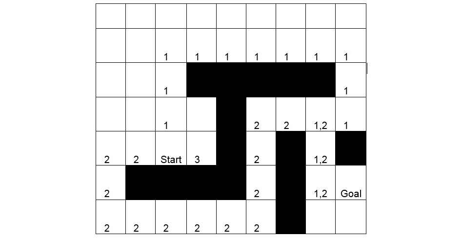
Figure 2.4: Shortest pathfinding game board with utilities
Exercise 6: Finding the Shortest Path to Reach a Goal
The steps to find the shortest path are as follows:
- Describe the board, the initial state, and the final state using Python. Create a function that returns a list of possible successor states.
- We will use tuples, where the first coordinate denotes the row number from 1 to 7, and the second coordinate denotes the column number from 1 to 9:
size = (7, 9)
start = (5, 3)
end = (6, 9)
obstacles = {
(3, 4), (3, 5), (3, 6), (3, 7), (3, 8),
(4, 5),
(5, 5), (5, 7), (5, 9),
(6, 2), (6, 3), (6, 4), (6, 5), (6, 7),
(7, 7)
}
- We will use array comprehension to generate the successor states in the following way. We move one left and one right from the current column, as long as we stay on the board. We move one up and one down from the current row, as long as we stay on the board. We take the new coordinates, generate all four possible tuples, and filter the results so that the new states can't be in the Obstacles list. It also makes sense to exclude moves that return to a field we had visited before to avoid infinite loops:
def successors(state, visited_nodes):
(row, col) = state
(max_row, max_col) = size
succ_states = []
if row > 1:
succ_states += [(row-1, col)]
if col > 1:
succ_states += [(row, col-1)]
if row < max_row:
succ_states += [(row+1, col)]
if col < max_col:
succ_states += [(row, col+1)]
return [s for s in succ_states if s not in visited_nodes if s not in obstacles]
Exercise 7: Finding the Shortest Path Using BFS
To find the shortest path, follow these steps:
Find the shortest path by using the BFS algorithm.
Recall the basic BFS implementation.
- We have to modify this implementation to include the cost. Let's measure the cost:
import math
def initialize_costs(size, start):
(h, w) = size
costs = [[math.inf] * w for i in range(h)]
(x, y) = start
costs[x-1][y-1] = 0
return costs
def update_costs(costs, current_node, successor_nodes):
new_cost = costs[current_node[0]-1][current_node[1]-1] + 1
for (x, y) in successor_nodes:
costs[x-1][y-1] = min(costs[x-1][y-1], new_cost)
def bfs_tree(node):
nodes_to_visit = [node]
visited_nodes = []
costs = initialize_costs(size, start)
while len(nodes_to_visit) > 0:
current_node = nodes_to_visit.pop(0)
visited_nodes.append(current_node)
successor_nodes = successors(current_node, visited_nodes)
update_costs(costs, current_node, successor_nodes)
nodes_to_visit.extend(successor_nodes)
return costs
bfs_tree(start)
- The output will be as follows:
[[6, 5, 4, 5, 6, 7, 8, 9, 10],
[5, 4, 3, 4, 5, 6, 7, 8, 9],
[4, 3, 2, inf, inf, inf, inf, inf, 10],
[3, 2, 1, 2, inf, 12, 13, 12, 11],
[2, 1, 0, 1, inf, 11, inf, 13, inf],
[3, inf, inf, inf, inf, 10, inf, 14, 15],
[4, 5, 6, 7, 8, 9, inf, 15, 16]]
- You can see that a simple BFS algorithm successfully determines the cost from the start node to any nodes, including the target node. Let's measure the number of steps required to find the goal node:
def bfs_tree_verbose(node):
nodes_to_visit = [node]
visited_nodes = []
costs = initialize_costs(size, start)
step_counter = 0
while len(nodes_to_visit) > 0:
step_counter += 1
current_node = nodes_to_visit.pop(0)
visited_nodes.append(current_node)
successor_nodes = successors(current_node, visited_nodes)
update_costs(costs, current_node, successor_nodes)
nodes_to_visit.extend(successor_nodes)
if current_node == end:
print(
'End node has been reached in ',
step_counter, '
steps'
)
return costs
return costs
bfs_tree_verbose(start)
- The end node has been reached in 110 steps:
[[6, 5, 4, 5, 6, 7, 8, 9, 10],
[5, 4, 3, 4, 5, 6, 7, 8, 9],
[4, 3, 2, inf, inf, inf, inf, inf, 10],
[3, 2, 1, 2, inf, 12, 13, 12, 11],
[2, 1, 0, 1, inf, 11, inf, 13, inf],
[3, inf, inf, inf, inf, 10, inf, 14, 15],
[4, 5, 6, 7, 8, 9, inf, 15, 16]]
We will now learn an algorithm that can find the shortest path from the start node to the goal node: the A* algorithm.
Introducing the A* Algorithm
A* is a complete and optimal heuristic search algorithm that finds the shortest possible path between the current game state and the winning state. The definition of complete and optimal in this state are as follows:
- Complete means that A* always finds a solution.
- Optimal means that A* will find the best solution.
To set up the A* algorithm, we need the following:
- An initial state
- A description of the goal states
- Admissible heuristics to measure progress toward the goal state
- A way to generate the next steps toward the goal
Once the setup is complete, we execute the A* algorithm using the following steps on the initial state:
- We generate all possible next steps.
- We store these children in the order of their distance from the goal.
- We select the child with the best score first and repeat these three steps on the child with the best score as the initial state. This is the shortest path to get to a node from the starting node.
distance_from_end( node ) is an admissible heuristic estimation showing how far we are from the goal node.
In pathfinding, a good heuristic can be the Euclidean distance. If the current node is (x, y) and the goal node is (u, v), then:
distance_from_end( node ) = sqrt( abs( x – u ) ** 2 + abs( y – v ) ** 2 )
Where:
- sqrt is the square root function. Don't forget to import it from the math library.
- abs is the absolute value function. abs( -2 ) = abs( 2 ) = 2.
- x ** 2 is x raised to the second power.
We will use the distance_from_start matrix to store the distances from the start node. In the algorithm, we will refer to this costs matrix as distance_from_start( n1 ). For any node, n1, that has coordinates (x1, y1), this distance is equivalent to distance_from_start[x1][y1].
We will use the succ( n ) notation to generate a list of successor nodes from n.
Let's see the pseudo-code of the algorithm:
frontier = [start], internal = {}
# Initialize the costs matrix with each cell set to infinity.
# Set the value of distance_from_start(start) to 0.
while frontier is not empty:
# notice n has the lowest estimated total
# distance between start and end.
n = frontier.pop()
# We'll learn later how to reconstruct the shortest path
if n == end:
return the shortest path.
internal.add(n)
for successor s in succ(n):
if s in internal:
continue # The node was already examined
new_distance = distance_from_start(n) + distance(n, s)
if new_distance >= distance_from_start(s):
# This path is not better than the path we have
# already examined.
continue
if s is a member of frontier:
update the priority of s
else:
Add s to frontier.
Regarding the retrieval of the shortest path, we can make use of the costs matrix. This matrix contains the distance of each node on the path from the start node. As cost always decreases when walking backward, all we need to do is start with the end node and walk backward greedily toward decreasing costs:
path = [end_node], distance = get_distance_from_start( end_node )
while the distance of the last element in the path is not 0:
for each neighbor of the last node in path:
new_distance = get_distance_from_start( neighbor )
if new_distance < distance:
add neighbor to path, and break out from the for loop
return path
A* shines when we have one Start state and one Goal state. The complexity of the A* algorithm is O( E ), where E stands for all possible edges in the field. In our example, we have up to four edges leaving any node: up, down, left, and right.
Note
To sort the frontier list in the proper order, we must use a special Python data structure: a priority queue.
# Import heapq to access the priority queue
import heapq
# Create a list to store the data
data = []
# Use heapq.heappush to push (priorityInt, value) pairs to the queue
heapq.heappush(data, (2, 'first item'))
heapq.heappush(data, (1, 'second item'))
# The tuples are stored in data in the order of ascending priority
[(1, 'second item'), (2, 'first item')]
# heapq.heappop pops the item with the lowest score from the queue
heapq.heappop(data)
The output is as follows:
(1, 'second item')
# data still contains the second item
data
The output is as follows:
[(2, 'first item')]
Why is it important that the heuristic used by the algorithm is admissible?
Because this is how we guarantee the optimal nature of the algorithm. For any node x, we are measuring the sum of the following: The distances from the start node to x The estimated distance from x to the end node. If the estimation never overestimates the distance from x to the end node, we will never overestimate the total distance. Once we are at the goal node, our estimation is zero, and the total distance from the start to the end becomes an exact number.
We can be sure that our solution is optimal because there are no other items in the priority queue that have a lower estimated cost. Given that we never overestimate our costs, we can be sure that all of the nodes in the frontier of the algorithm have either similar total costs or higher total costs than the path we found.
Implement the A* algorithm to find the path with the lowest cost in the following game field:
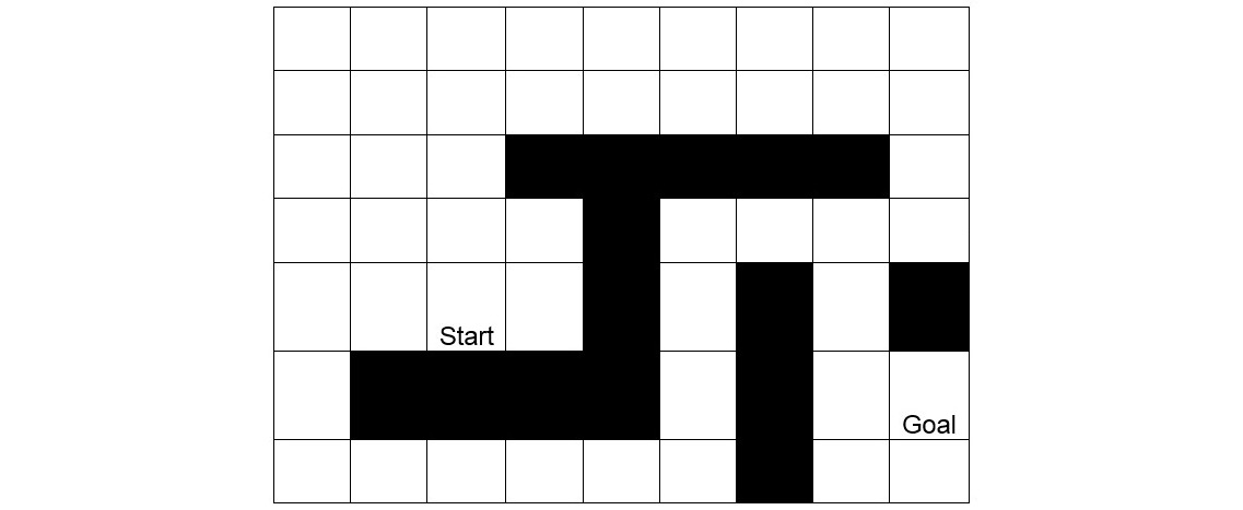
Figure 2.5: Shortest pathfinding game board
We'll reuse the initialization code from the game-modeling exercise:
import math
import heapq
size = (7, 9)
start = (5, 3)
end = (6, 9)
obstacles = {
(3, 4), (3, 5), (3, 6), (3, 7), (3, 8),
(4, 5),
(5, 5), (5, 7), (5, 9),
(6, 2), (6, 3), (6, 4), (6, 5), (6, 7),
(7, 7)
}
# Returns the successor nodes of State, excluding nodes in VisitedNodes
def successors(state, visited_nodes):
(row, col) = state
(max_row, max_col) = size
succ_states = []
if row > 1:
succ_states += [(row-1, col)]
if col > 1:
succ_states += [(row, col-1)]
if row < max_row:
succ_states += [(row+1, col)]
if col < max_col:
succ_states += [(row, col+1)]
return [s for s in succ_states if s not in visited_nodes if s not in obstacles]
We have also written code to initialize the cost matrix:
import math
def initialize_costs(size, start):
costs = [[math.inf] * 9 for i in range(7)]
(x, y) = start
costs[x-1][y-1] = 0
return costs
We will omit the function to update costs because we will do so inside the A* algorithm:
Let's initialize the A* algorithm's frontier and internal lists. For frontier, we will use a Python PriorityQueue. Do not directly execute this code, because we will use these four lines inside the A* search function:
frontier = []
internal = set()
heapq.heappush(frontier, (0, start))
costs = initialize_costs(size, start)
Now it is time to implement a heuristic function that measures the distance between the current node and the goal node using the algorithm we saw in the theory section:
def distance_heuristic(node, goal):
(x, y) = node
(u, v) = goal
return math.sqrt(abs(x - u) ** 2 + abs(y - v) ** 2)
The last step is the translation of the A* algorithm into the functioning code:
def astar(start, end):
frontier = []
internal = set()
heapq.heappush(frontier, (0, start))
costs = initialize_costs(size, start)
def get_distance_from_start(node):
return costs[node[0] - 1][node[1] - 1]
def set_distance_from_start(node, new_distance):
costs[node[0] - 1][node[1] - 1] = new_distance
while len(frontier) > 0:
(priority, node) = heapq.heappop(frontier)
if node == end:
return priority
internal.add(node)
successor_nodes = successors(node, internal)
for s in successor_nodes:
new_distance = get_distance_from_start(node) + 1
if new_distance < get_distance_from_start(s):
set_distance_from_start(s, new_distance)
# Filter previous entries of s
frontier = [n for n in frontier if s != n[1]]
heapq.heappush(frontier, (
new_distance + distance_heuristic(s, end), s
)
)
astar(start, end)
15.0
There are a few differences between our implementation and the original algorithm:
We defined a distance_from_start function to make it easier and more semantic to access the costs matrix. Note that we number the node indices starting with 1, while in the matrix, indices start with zero. Therefore, we subtract 1 from the node values to get the indices.
When generating the successor nodes, we automatically ruled out nodes that are in the Internal set. successors = succ(node, internal) makes sure that we only get the neighbors whose examination is not yet closed, meaning that their score is not necessarily optimal.
As a consequence, we may skip the step check, as internal nodes will never end up in succ( n ).
As we are using a priority queue, we have to determine the estimated priority of node s before inserting it. We will only insert the node to frontier, though, if we know that this node does not have an entry with a lower score.
It may happen that node s is already in the frontier queue with a higher score. In this case, we remove this entry before inserting it to the right place in the priority queue. When we find the end node, we simply return the length of the shortest path instead of the path itself.
To get a bit more information on the execution, let's print this information to the console. To follow what the A* algorithm does, execute this code and study the logs:
def astar_verbose(start, end):
frontier = []
internal = set()
heapq.heappush(frontier, (0, start))
costs = initialize_costs(size, start)
def get_distance_from_start(node):
return costs[node[0] - 1][node[1] - 1]
def set_distance_from_start(node, new_distance):
costs[node[0] - 1][node[1] - 1] = new_distance
steps = 0
while len(frontier) > 0:
steps += 1
print('step ', steps, '. frontier: ', frontier)
(priority, node) = heapq.heappop(frontier)
print(
'node ',
node,
'has been popped from frontier with priority',
priority
)
if node == end:
print('Optimal path found. Steps: ', steps)
print('Costs matrix: ', costs)
return priority
internal.add(node)
successor_nodes = successors(node, internal)
print('successor_nodes', successor_nodes)
for s in successor_nodes:
new_distance = get_distance_from_start(node) + 1
print(
's:',
s,
'new distance:',
new_distance,
' old distance:',
get_distance_from_start(s)
)
if new_distance < get_distance_from_start(s):
set_distance_from_start(s, new_distance)
# Filter previous entries of s
frontier = [n for n in frontier if s != n[1]]
new_priority = new_distance + distance_heuristic(s, end)
heapq.heappush(frontier, (new_priority, s))
print(
'Node',
s,
'has been pushed to frontier with priority',
new_priority
)
print('Frontier', frontier)
print('Internal', internal)
print(costs)
astar_verbose(start, end)
The output is as follows:
step 1 . Frontier: [(0, (5, 3))]
Node (5, 3) has been popped from Frontier with priority 0
successors [(4, 3), (5, 2), (5, 4)]
s: (4, 3) new distance: 1 old distance: inf
Node (4, 3) has been pushed to Frontier with priority 7.324555320336759
s: (5, 2) new distance: 1 old distance: inf
Node (5, 2) has been pushed to Frontier with priority 8.071067811865476
s: (5, 4) new distance: 1 old distance: inf
Node (5, 4) has been pushed to Frontier with priority 6.0990195135927845
step 2 . Frontier: [(6.0990195135927845, (5, 4)), (8.071067811865476, (5, 2)), (7.324555320336759, (4, 3))]
Node (5, 4) has been popped from Frontier with priority 6.0990195135927845
successors [(4, 4)]
s: (4, 4) new distance: 2 old distance: inf
Node (4, 4) has been pushed to Frontier with priority 7.385164807134504
…
step 42 . Frontier: [(15.0, (6, 8)), (15.60555127546399, (4, 6)), (15.433981132056603, (1, 1)), (15.82842712474619, (4, 7))]
Node (6, 8) has been popped from Frontier with priority 15.0
successors [(7, 8), (6, 9)]
s: (7, 8) new distance: 15 old distance: inf
Node (7, 8) has been pushed to Frontier with priority 16.414213562373096
s: (6, 9) new distance: 15 old distance: inf
Node (6, 9) has been pushed to Frontier with priority 15.0
step 43 . Frontier: [(15.0, (6, 9)), (15.433981132056603, (1, 1)), (15.82842712474619, (4, 7)), (16.414213562373096, (7, 8)), (15.60555127546399, (4, 6))]
Node (6, 9) has been popped from Frontier with priority 15.0
Optimal path found. Steps: 43
Costs matrix: [[6, 5, 4, 5, 6, 7, 8, 9, 10], [5, 4, 3, 4, 5, 6, 7, 8, 9], [4, 3, 2, inf, inf, inf, inf, inf, 10], [3, 2, 1, 2, inf, 12, 13, 12, 11], [2, 1, 0, 1, inf, 11, inf, 13, inf], [3, inf, inf, inf, inf, 10, inf, 14, 15], [4, 5, 6, 7, 8, 9, inf, 15, inf]]
We have seen that the A * search returns the right values. The question is, how can we reconstruct the whole path?
Remove the print statements from the code for clarity and continue with the A* algorithm that we implemented in step 4. Instead of returning the length of the shortest path, we have to return the path itself. We will write a function that extracts this path by walking backward from the end node, analyzing the costs matrix. Do not define this function globally yet. We will define it as a local function in the A* algorithm that we created previously:
def get_shortest_path(end_node):
path = [end_node]
distance = get_distance_from_start(end_node)
while distance > 0:
for neighbor in successors(path[-1], []):
new_distance = get_distance_from_start(neighbor)
if new_distance < distance:
path += [neighbor]
distance = new_distance
break # for
return path
Now that we know how to deconstruct the path, let's return it inside the A* algorithm:
def astar_with_path(start, end):
frontier = []
internal = set()
heapq.heappush(frontier, (0, start))
costs = initialize_costs(size, start)
def get_distance_from_start(node):
return costs[node[0] - 1][node[1] - 1]
def set_distance_from_start(node, new_distance):
costs[node[0] - 1][node[1] - 1] = new_distance
def get_shortest_path(end_node):
path = [end_node]
distance = get_distance_from_start(end_node)
while distance > 0:
for neighbor in successors(path[-1], []):
new_distance = get_distance_from_start(neighbor)
if new_distance < distance:
path += [neighbor]
distance = new_distance
break # for
return path
while len(frontier) > 0:
(priority, node) = heapq.heappop(frontier)
if node == end:
return get_shortest_path(end)
internal.add(node)
successor_nodes = successors(node, internal)
for s in successor_nodes:
new_distance = get_distance_from_start(node) + 1
if new_distance < get_distance_from_start(s):
set_distance_from_start(s, new_distance)
# Filter previous entries of s
frontier = [n for n in frontier if s != n[1]]
heapq.heappush(frontier, (
new_distance + distance_heuristic(s, end), s
)
)
astar_with_path( start, end )
The output is as follows:
[(6, 9),
(6, 8),
(5, 8),
(4, 8),
(4, 9),
(3, 9),
(2, 9),
(2, 8),
(2, 7),
(2, 6),
(2, 5),
(2, 4),
(2, 3),
(3, 3),
(4, 3),
(5, 3)]
Technically, we do not need to reconstruct the path from the costs matrix. We could record the parent node of each node in a matrix, and simply retrieve the coordinates to save a bit of searching.
A* Search in Practice Using the simpleai Library
The simpleai library is available on GitHub, and contains many popular AI tools and techniques.
Note
You can access the library at https://github.com/simpleai-team/simpleai. The documentation of the Simple AI library can be accessed here: http://simpleai.readthedocs.io/en/latest/.To access the simpleai library, first you have to install it:
pip install simpleai
Once simpleai has been installed, you can import classes and functions from the simpleai library in the Jupyter QtConsole of Python:
from simpleai.search import SearchProblem, astar
Search Problem gives you a frame for defining any search problems. The astar import is responsible for executing the A* algorithm inside the search problem.
For simplicity, we have not used classes in the previous code examples to focus on the algorithms in a plain old style without any clutter. The simpleai library will force us to use classes, though.
To describe a search problem, you need to provide the following:
- constructor: This initializes the state space, thus describing the problem. We will make the Size, Start, End, and Obstacles values available in the object by adding it to these as properties. At the end of the constructor, don't forget to call the super constructor, and don't forget to supply the initial state.
- actions( state ): This returns a list of actions that we can perform from a given state. We will use this function to generate the new states. Semantically, it would make more sense to create action constants such as UP, DOWN, LEFT, and RIGHT, and then interpret these action constants as a result. However, in this implementation, we will simply interpret an action as "move to (x, y)", and represent this command as (x, y). This function contains more-or-less the logic that we implemented in the succ function before, except that we won't filter the result based on a set of visited nodes.
- result( state0, action): This returns the new state of action applied on the state0.
- is_goal( state ): This returns true if the state is a goal state. In our implementation, we will have to compare the state to the end state coordinates.
- cost( self, state, action, newState ): This is the cost of moving from state to newState via action. In our example, the cost of a move is uniformly 1:
import math
from simpleai.search import SearchProblem, astar
class ShortestPath(SearchProblem):
def __init__(self, size, start, end, obstacles):
self.size = size
self.start = start
self.end = end
self.obstacles = obstacles
super(ShortestPath, self).__init__(initial_state=self.start)
def actions(self, state):
(row, col) = state
(max_row, max_col) = self.size
succ_states = []
if row > 1:
succ_states += [(row-1, col)]
if col > 1:
succ_states += [(row, col-1)]
if row < max_row:
succ_states += [(row+1, col)]
if col < max_col:
succ_states += [(row, col+1)]
return [s for s in succ_states if s not in self._obstacles]
def result(self, state, action):
return action
def is_goal(self, state):
return state == end
def cost(self, state, action, new_state):
return 1
def heuristic(self, state):
(x, y) = state
(u, v) = self.end
return math.sqrt(abs(x-u) ** 2 + abs(y-v) ** 2)
size = (7, 9)
start = (5, 3)
end = (6, 9)
obstacles = {
(3, 4), (3, 5), (3, 6), (3, 7), (3, 8),
(4, 5),
(5, 5), (5, 7), (5, 9),
(6, 2), (6, 3), (6, 4), (6, 5), (6, 7),
(7, 7)
}
searchProblem = ShortestPath(Size, Start, End, Obstacles)
result = astar( searchProblem, graph_search=True )
result
Node <(6, 9)>
result.path()
[(None, (5, 3)),
((4, 3), (4, 3)),
((3, 3), (3, 3)),
((2, 3), (2, 3)),
((2, 4), (2, 4)),
((2, 5), (2, 5)),
((2, 6), (2, 6)),
((2, 7), (2, 7)),
((2, 8), (2, 8)),
((2, 9), (2, 9)),
((3, 9), (3, 9)),
((4, 9), (4, 9)),
((4, 8), (4, 8)),
((5, 8), (5, 8)),
((6, 8), (6, 8)),
((6, 9), (6, 9))]
The simpleai library made the search description a lot easier than the manual implementation. All we need to do is define a few basic methods, and then we have access to an effective search implementation.
Game AI with the Minmax Algorithm and Alpha-Beta Pruning
In the first two topics, we saw how hard it was to create a winning strategy for a simple game such as Tic-Tac-Toe. The last topic introduced a few structures for solving search problems with the A* algorithm. We also saw that tools such as the simpleai library help us reduce the effort we put in to describe a task with code.
We will use all of this knowledge to supercharge our game AI skills and solve more complex problems.
Search Algorithms for Turn-Based Multiplayer Games
Turn-based multiplayer games such as Tic-Tac-Toe are similar to pathfinding problems. We have an initial state, and we have a set of end states, where we win the game.
The challenge with turn-based multiplayer games is the combinatoric explosion of the opponent's possible moves. This difference justifies treating turn-based games differently than a regular pathfinding problem.
For instance, in the Tic-Tac-Toe game, from an empty board, we can select one of the nine cells and place our sign there, assuming we start the game. Let's denote this algorithm with the function succ, symbolizing the creation of successor states. Consider we have the initial state denoted by Si.
succ(Si) returns [ S1, S2, ..., Sn ], where S1, S2, ..., Sn are successor states:

Figure 2.6: Tree diagram denoting the successor states of the function
Then, the opponent also makes a move, meaning that from each possible state, we have to examine even more states:
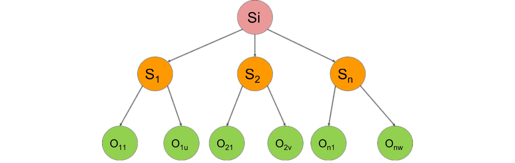
Figure 2.7: Tree diagram denoting parent-successor relationships
The expansion of possible future states stops in one of two cases:
- The game ends
- Due to resource limitations, it is not worth explaining any more moves beyond a certain depth for a state with a certain utility
Once we stop expanding, we have to make a static heuristic evaluation of the state. This is exactly what we did in the first two topics, when choosing the best move; however, we never considered future states.
Therefore, even though our algorithm became more and more complex, without using the knowledge of possible future states, we had a hard time detecting whether our current move would likely be a winner or a loser. The only way for us to take control of the future was to change our heuristic knowing how many games we would win, lose, or tie in the future. We could either maximize our wins or minimize our losses. We still didn't dig deeply enough to see whether our losses could have been avoided through smarter play on the AI's end.
All of these problems can be avoided by digging deeper into future states and recursively evaluating the utility of the branches. To consider future states, we will learn the Minmax algorithm and its variant, the Negamax algorithm.
The Minmax Algorithm
Suppose there's a game where a heuristic function can evaluate a game state from the perspective of the AI player. For instance, we used a specific evaluation for the Tic-Tac-Toe exercise:
- +1,000 points for a move that won the game
- +100 points for a move preventing the opponent from winning the game
- +10 points for a move creating two in a row, column, or diagonal
- +1 point for a move creating one in a row, column, or diagonal
This static evaluation is very easy to implement on any node. The problem is, as we go deep into the tree of all possible future states, we don't know what to do with these scores yet. This is where the Minmax algorithm comes into play.
Suppose we construct a tree with each possible move that could be performed by each player up to a certain depth. At the bottom of the tree, we evaluate each option. For the sake of simplicity, let's assume that we have a search tree that looks as follows:
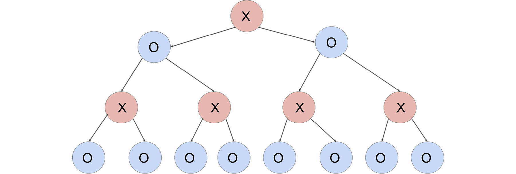
Figure 2.8: Example of search tree up to a certain depth
The AI plays with X, and the player plays with O. A node with X means that it's X's turn to move. A node with O means it's O's turn to act.
Suppose there are all O leaves at the bottom of the tree, and we didn't compute any more values because of resource limitations. Our task is to evaluate the utility of the leaves:
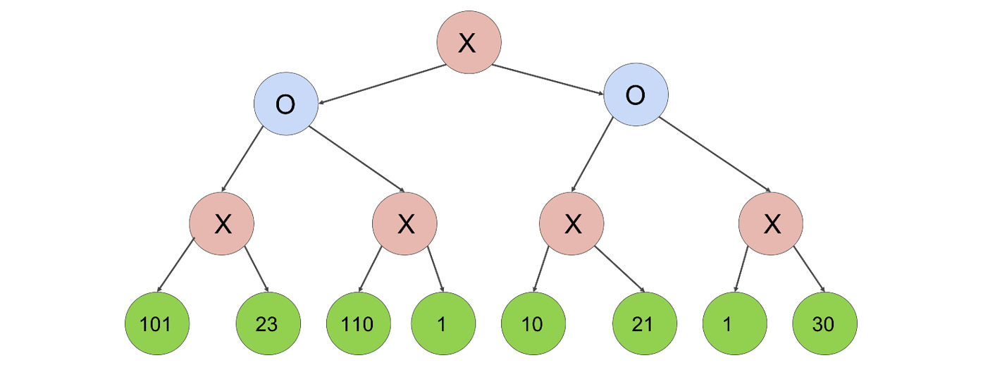
Figure 2.9: Example of search tree with possible moves
We have to select the best possible move from our perspective, because our goal is to maximize the utility of our move. This aspiration to maximize our gains represents the Max part in the Minmax algorithm:
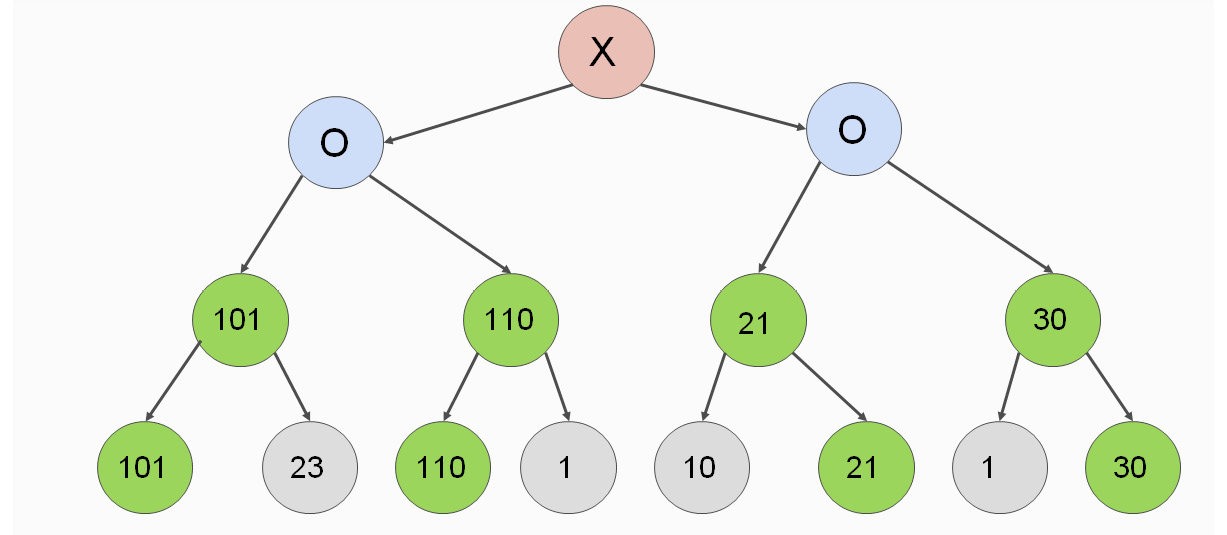
Figure 2.10: Example of search tree with best possible move
If we move one level higher, it is our opponent's turn to act. Our opponent picks the value that is the least beneficial to us. This is because our opponent's job is to minimize our chances of winning the game. This is the Min part of the Minmax algorithm:
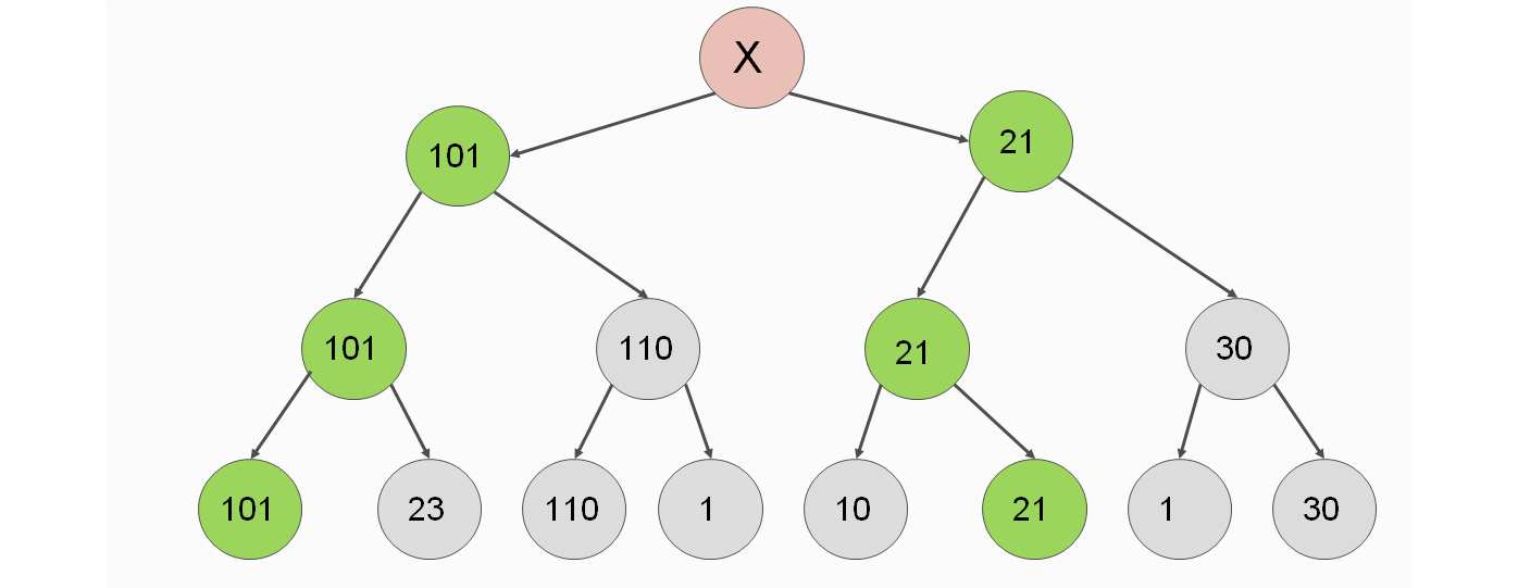
Figure 2.11: Minimizing the chances of winning the game
At the top, we can choose between a move with utility 101 and another move with utility 21. As we are maximizing our value, we should pick 101.
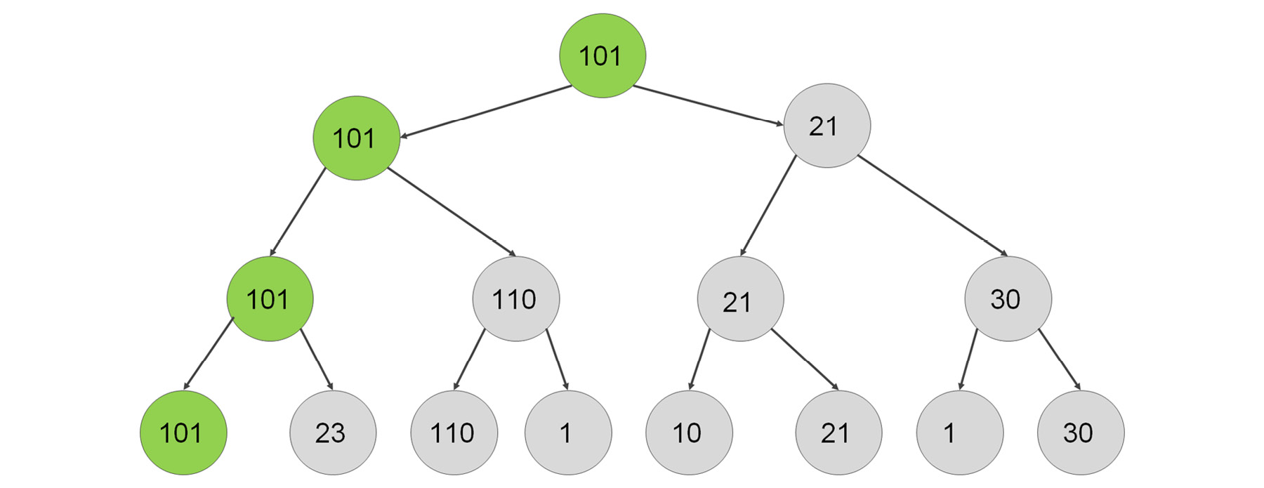
Figure 2.12: Maximizing the chances of winning the game
Let's see how we can implement this idea:
def min_max( state, depth, is_maximizing):
if depth == 0 or is_end_state( state ):
return utility( state )
if is_maximizing:
utility = 0
for s in successors( state ):
score = MinMax( s, depth - 1, false )
utility = max( utility, score )
return utility
else
utility = infinity
for s in successors( state ):
score = MinMax( s, depth - 1, true )
utility = min( utility, score )
return utility
This is the Minmax algorithm. We evaluate the leaves from our perspective. Then, from the bottom-up, we apply a recursive definition:
- Our opponent plays optimally by selecting the worst possible node from our perspective.
- We play optimally by selecting the best possible node from our perspective.
We need a few more considerations to understand the application of the Minmax algorithm on the Tic-Tac-Toe game:
- is_end_state is a function that determines whether the state should be evaluated instead of digging deeper, either because the game has ended, or because the game is about to end using forced moves. Using our utility function, it is safe to say that as soon as we reach a score of 1,000 or higher, we have effectively won the game. Therefore, is_end_state can simply check the score of a node and determine whether we need to dig deeper.
- Although the successors function only depends on the state, it is practical to pass the information of whose turn it is to make a move. Therefore, don't hesitate to add an argument if needed; you don't have to follow the pseudocode.
- We want to minimize our efforts in implementing the Minmax algorithm. For this reason, we will evaluate existing implementations of the algorithm, and we will also simplify the duality of the description of the algorithm in the rest of this topic.
- The suggested utility function is quite accurate compared to utility functions that we could be using in this algorithm. In general, the deeper we go, the less accurate our utility function has to be. For instance, if we could go nine steps deep into the Tic-Tac-Toe game, all we would need to do is award 1 point for a win, zero for a draw, and -1 point for a loss. Given that, in nine steps, the board is complete, and we have all of the necessary information to make the evaluation. If we could only look four steps deep, this utility function would be completely useless at the start of the game, because we need at least five steps to win the game.
- The Minmax algorithm could be optimized further by pruning the tree. Pruning is an act where we get rid of branches that don't contribute to the end result. By eliminating unnecessary computations, we save precious resources that could be used to go deeper into the tree.
Optimizing the Minmax Algorithm with Alpha-Beta Pruning
The last consideration in the previous thought process primed us to explore possible optimizations on reducing the search space by focusing our attention on nodes that matter.
There are a few constellations of nodes in the tree, where we can be sure that the evaluation of a subtree does not contribute to the end result. We will find, examine, and generalize these constellations to optimize the Minmax algorithm.
Let's examine pruning through the previous example of nodes:
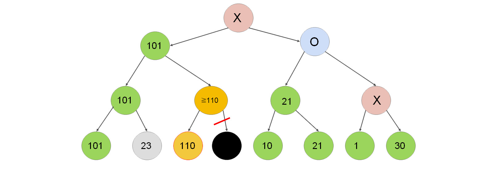
Figure 2.13: Search tree demonstrating pruning nodes
After computing the nodes with values 101, 23, and 110, we can conclude that two levels above, the value 101 will be chosen. Why?
- Suppose X <= 110. Then the maximum of 110 and X will be chosen, which is 110, and X will be omitted.
- Suppose X > 110. Then the maximum of 110 and X is X. One level above, the algorithm will choose the lowest value out of the two. The minimum of 101 and X will always be 101, because X > 110. Therefore, X will be omitted a level above.
This is how we prune the tree.
On the right-hand side, suppose we computed branches 10 and 21. Their maximum is 21. The implication of computing these values is that we can omit the computation of nodes Y1, Y2, and Y3, and we will know that the value of Y4 is less than or equal to 21. Why?
The minimum of 21 and Y3 is never greater than 21. Therefore, Y4 will never be greater than 21.
We can now choose between a node with utility 101, and another node with a maximal utility of 21. It is obvious that we have to choose the node with utility 101.
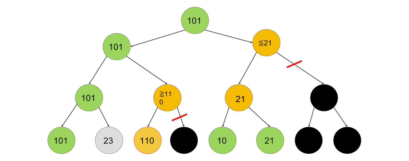
Figure 2.14: Example of pruning a tree
This is the idea behind alpha-beta pruning. We prune subtrees that we know are not going to be needed.
Let's see how we can implement alpha-beta pruning in the Minmax algorithm.
First, we will add an alpha and a beta argument to the argument list of Minmax:
def min_max(state, depth, is_maximizing, alpha, beta):
if depth == 0 or is_end_state(state):
return utility(state)
if is_maximizing:
utility = 0
for s in successors(state):
score = MinMax(s, depth - 1, false, alpha, beta)
utility = max(utility, score)
return utility
else
utility = infinity
for s in successors(state):
score = MinMax(s, depth - 1, true, alpha, beta)
utility = min(utility, score)
return utility
For the isMaximizing branch, we calculate the new alpha score, and break out of the loop whenever beta <= alpha:
def min_max(state, depth, is_maximizing, alpha, beta):
if depth == 0 or is_end_state(state):
return utility(state)
if is_maximizing:
utility = 0
for s in successors(state):
score = MinMax(s, depth - 1, false, alpha, beta)
utility = max(utility, score)
alpha = max(alpha, score)
if beta <= alpha:
break
return utility
else
utility = infinity
for s in successors(state):
score = MinMax(s, depth - 1, true, alpha, beta)
utility = min(utility, score)
return utility
We need to do the dual for the minimizing branch:
def min_max(state, depth, is_maximizing, alpha, beta):
if depth == 0 or is_end_state( state ):
return utility(state)
if is_maximizing:
utility = 0
for s in successors(state):
score = min_max(s, depth - 1, false, alpha, beta)
utility = max(utility, score)
alpha = max(alpha, score)
if beta <= alpha: break
return utility
else
utility = infinity
for s in successors(state):
score = min_max(s, depth - 1, true, alpha, beta)
utility = min(utility, score)
beta = min(beta, score)
if beta <= alpha: break
return utility
We are done with the implementation. It is recommended that you mentally execute the algorithm on our example tree step-by-step to get a feel for the implementation.
One important piece is missing that's preventing us from doing the execution properly: the initial values for alpha and beta. Any number that's outside the possible range of utility values will do. We will use positive and negative infinity as initial values to call the Minmax algorithm:
alpha = infinity
beta = -infinity
DRYing up the Minmax Algorithm – The NegaMax Algorithm
The Minmax algorithm works great, especially with alpha-beta pruning. The only problem is that we have an if and an else branch in the algorithm that essentially negate each other.
As we know, in computer science, there is DRY code and WET code. DRY stands for Don't Repeat Yourself. Wet stands for We Enjoy Typing. When we write the same code twice, we double our chance of making a mistake while writing it. We also double our chances of each maintenance effort being executed in the future. Hence, it's better to reuse our code.
When implementing the Minmax algorithm, we always compute the utility of a node from the perspective of the AI player. This is why we have to have a utility-maximizing branch and a utility-minimizing branch in the implementations that are dual in nature. As we prefer clean code that describes the problem only once, we could get rid of this duality by changing the point of view of the evaluation.
Whenever the AI player's turn comes, nothing changes in the algorithm.
Whenever the opponent's turn comes, we negate the perspective. Minimizing the AI player's utility is equivalent to maximizing the opponent's utility.
This simplifies the Minmax algorithm:
def Negamax(state, depth, is_players_point_of_view):
if depth == 0 or is_end_state(state):
return utility(state, is_players_point_of_view)
utility = 0
for s in successors(state):
score = Negamax(s,depth-1,not is_players_point_of_view)
return score
There are necessary conditions for using the Negamax algorithm: the evaluation of the board state has to be symmetric. If a game state is worth +20 from the first player's perspective, it is worth -20 from the second player's perspective. Therefore, we often normalize the scores around zero.
Using the EasyAI Library
We have seen the simpleai library that helped us execute searches on pathfinding problems. We will now use the EasyAI library, which can easily handle AI search on two player games, reducing the implementation of the Tic-Tac-Toe problem to writing a few functions on scoring the utility of a board and determining when the game ends.
You can read the documentation of the library on GitHub at https://github.com/Zulko/easyAI.
To install the EasyAI library, run the following command:
pip install easyai
Note
As always, if you are using Anaconda, you must execute this command in the Anaconda prompt, and not in the Jupyter QtConsole.
Once EasyAI is available, it makes sense to follow the structure of the documentation to describe the Tic-Tac-Toe problem.This implementation was taken from https://zulko.github.io/easyAI/examples/games.html, where the Tic-Tac-Toe problem is described in a compact and elegant way:
from easyAI import TwoPlayersGame
from easyAI.Player import Human_Player
class TicTacToe( TwoPlayersGame ):
""" The board positions are numbered as follows:
7 8 9
4 5 6
1 2 3
"""
def __init__(self, players):
self.players = players
self.board = [0 for i in range(9)]
self.nplayer = 1 # player 1 starts.
def possible_moves(self):
return [i+1 for i,e in enumerate(self.board) if e==0]
def make_move(self, move):
self.board[int(move)-1] = self.nplayer
def unmake_move(self, move): # optional method (speeds up the AI)
self.board[int(move)-1] = 0
def lose(self):
""" Has the opponent "three in line ?" """
return any( [all([(self.board[c-1]== self.nopponent)
for c in line])
for line in [[1,2,3],[4,5,6],[7,8,9],
[1,4,7],[2,5,8],[3,6,9],
[1,5,9],[3,5,7]]])
def is_over(self):
return (self.possible_moves() == []) or self.lose()
def show(self):
print (' '+' '.join([
' '.join([['.','O','X'][self.board[3*j+i]]
for i in range(3)])
for j in range(3)]) )
def scoring(self):
return -100 if self.lose() else 0
if __name__ == "__main__":
from easyAI import AI_Player, Negamax
ai_algo = Negamax(6)
TicTacToe( [Human_Player(),AI_Player(ai_algo)]).play()
In this implementation, the computer player never loses thanks to the Negamax algorithm exploring the search criterion in a depth of 6.
Notice the simplicity of the scoring function. Wins or losses can guide the AI player to reach the goal of never losing a game.
Activity 4: Connect Four
In this section, we will practice using the EasyAI library and develop a heuristic. We will be using the game Connect 4 for this. The game board is seven cells wide and seven cells high. When you make a move, you can only select the column in which you drop your token. Then, gravity pulls the token down to the lowest possible empty cell. Your objective is to connect four of your own tokens horizontally, vertically, or diagonally, before your opponent does, or you run out of empty spaces. The rules of the game can be found at https://en.wikipedia.org/wiki/Connect_Four.
We can leave a few functions from the definition intact. We have to implement the following methods:
- __init__
- possible_moves
- make_move
- unmake_move (optional)
- lose
- show
- We will reuse the basic scoring function from Tic-Tac-Toe. Once you test out the game, you will see that the game is not unbeatable, but plays surprisingly well, even though we are only using basic heuristics.
- Then, let's write the init method. We will define the board as a one-dimensional list, like the Tic-Tac-Toe example. We could use a two-dimensional list too, but modeling will not get much easier or harder. We will generate all of the possible winning combinations in the game and save them for future use.
- Let's handle the moves. The possible moves function is a simple enumeration. Notice that we are using column indices from 1 to 7 in the move names, because it is more convenient to start column indexing with 1 in the human player interface than with zero. For each column, we check whether there is an unoccupied field. If there is one, we will make the column a possible move.
- Making a move is similar to the possible moves function. We check the column of the move and find the first empty cell, starting from the bottom. Once we find it, we occupy it. You can also read the implementation of the dual of the make_move function: unmake_move. In the unmake_move function, we check the column from top to bottom, and we remove the move at the first non-empty cell. Notice that we rely on the internal representation of easyAi so that it does not undo moves that it has not made. If we didn't, this function would remove one of the other player's tokens without checking whose token was removed.
- As we already have the tuples that we have to check, we can mostly reuse the lose function from the Tic-Tac-Toe example.
- Our last task is to implement the show method that prints the board. We will reuse the Tic-Tac-Toe implementation and just change the variables.
- Now that all of the functions are complete, you can try out the example. Feel free to play a round or two against the opponent. You can see that the opponent is not perfect, but it plays reasonably well. If you have a strong computer, you can increase the parameter of the Negamax algorithm. I encourage you to come up with a better heuristic.
Note
The solution for this activity can be found on page 265.
Summary
In this chapter, we learned how to apply search techniques to play games.
First, we created a static approach that played the Tic-Tac-Toe game based on predefined rules without looking ahead. Then, we quantified these rules into a number we called heuristics. In the next topic, we learned how to use heuristics in the A* search algorithm to find an optimal solution to a problem.
Finally, we got to know the Minmax and the NegaMax algorithms so that the AI could win two-player games.
Now that you know the fundamentals of writing game AI, it is time to learn about a different field within artificial intelligence: machine learning. In the next chapter, you will learn about regression.