
12
Collaboration networks in the US Senate
The inner workings of legislatures are inherently difficult to investigate. Political scientists have been interested in collaborations among parliamentarians as explanatory factors in legislative behavior for decades. Scholars have encountered difficulties, however, in collecting comprehensive data over time to investigate patterns of cooperation. The advent of large-scale, machine-readable databases on legislative behavior have opened up promising new research avenues in this regard. Among these, scholars have considered the possibility of treating bill cosponsorships as proxies for legislative cooperation in the United States. We follow this lead and investigate who cooperates with whom in the US Senate.
Every bill that is introduced to the US Senate is tied to one senator as its main sponsor, but other senators are free to cosponsor a bill in order to support the bill's content—a common practice in senatorial procedures. In fact, in many instances, a bill will have numerous cosponsors. Several authors have recently begun to truly appreciate the network-like structure in bill cosponsorships that is best analyzed using network-analytic methodology.1 Using the rich and well accessible data source on bill cosigners provides researchers with an interesting insight into the black box of collaboration among senators. What is more, bill cosponsorships are moving targets. New proposals are constantly put on record. Being able to collect these data automatically provides researchers with a unique opportunity to consider structural changes in the networks as they are happening.
In this application, we generate the necessary data to replicate some of the analyses that have been put forward in recent years. For simplicity's sake, we only assemble data on bill cosponsorships for the US Senate in the 111th Congress, which was in session from 2009 to 2010. Sections 12.1 and 12.2 provide the technical details on how the underlying data sources are generated. Again, our focus in this chapter is on data gathering; hence, we only analyze the data with simple metrics. Section 12.3 gives a brief overview on how the data can be employed—both descriptively and in a basic network application. Section 12.4 concludes the chapter.
12.1 Information on the bills
Our first task is to assemble a list of all sponsors and cosponsors on each bill. To keep matters simple, we will only gather data for the 111th Senate, which ran from 2009 to 2010. As we are more interested in the process of data gathering than in the actual application, there is more than enough material in one senatorial term. Should you wish to analyze the data for an actual application, it is fairly straightforward to adapt the script to encompass more legislative periods.
Our specific goal in this section is to construct a matrix that holds information on whether a senator has sponsored, cosponsored, or not participated at all in a given bill. A mock example of the data structure is presented in Table 12.1. Storing the data in this format provides the greatest flexibility for subsequent analyses. We could, for example, be interested in analyzing which senator was better able to collect cosponsors, or we might want to analyze which Senators were often cosponsors on the same piece of legislation to find collaboration clusters in the Senate. We can easily rearrange the proposed table using the facilities of R without having to reassemble all the data from scratch if we tailor the table to a particular application from the start. Furthermore, this data matrix even allows performing an ideal point estimation (Alemán et al. 2009; Desposato et al. 2011; Peress 2010) that we will, however, not tackle in this chapter.
Table 12.1 Desired data structure for sponsorship matrix
| Senator A | Senator B | Senator C | ... | |
| S.1 | Cosponsor | Sponsor | Cosponsor | ... |
| S.2 | . | . | . | ... |
| S.3 | . | Cosponsor | Sponsor | ... |
| S.4 | . | . | Sponsor | ... |
| S.5 | . | . | . | ... |
| S.6 | Cosponsor | . | Cosponsor | ... |
| S.7 | Sponsor | . | . | ... |
| ⋮ | ⋮ | ⋮ | ⋮ | ⋱ |
The table displays a mock example of the dataset we wish to generate. The rows list each bill, the columns list each senator. The cells display whether a senator was the main sponsor of a bill (Sponsor), has cosponsored a bill (Cosponsor) or did not sign a bill at all (.).
Let us have a look at the database. Luckily, the bills of the US Congress are stored in a database that is relatively accessible at http://thomas.loc.gov.2 The first step in our web scraping exercise is an inspection of the way the data are stored. In order to be able to track the scraping procedure,
- Call http://thomas.loc.gov/home/thomas.php
- Go to “Try the Advanced Search”
- Click on “Browse Bills & Resolutions” right above it
- Select “111” at the top of the page
- On the resulting page click on “Senate Bills”
The resulting page holds the main information on the first 100 of 4059 bills proposed during the 111th Senate. Specifically, we see the title of the proposed bill, its sponsor, the number of cosponsors, and the latest major action for each item. Now click on Cosponsors of the first bill S.1. Apart from the previously mentioned elements, we additionally see a list of the bill's 17 cosponsors. This page holds all the information we are interested in for now which greatly facilitates our task. Check out the URL of the page—http://thomas.loc.gov/cgi-bin/bdquery/D?d111:1:./list/bss/d111SN.lst:@@@P. Despite its somewhat peculiar format the numerator of this piece of legislation, 1, is hidden right in the middle next to the senate term 111. To be sure, click on the NEXT:COSPONSORS button. Now the URL reads http://thomas.loc.gov/cgi-bin/bdquery/D?d111:2:./list/bss/d111SN.lst:@@@P:&summ2=m&. Disregarding the altered ending of the URL, we notice that the middle of the URL now reads 2 for the second bill in the 111th Senate.
As the attached ending is not a necessary prerequisite to get the information, we are looking for, but is rather added due to the referral from one site to the next, we can safely drop it. Choosing a random number, 42, we rewrite the original URL by hand to read http://thomas.loc.gov/cgi-bin/bdquery/D?d111:42:./list/bss/d111SN.lst:@@@P. Works like a charm. Now, in line with our rules of good practice in web scraping, we will download the web pages of all 4059 bills to our local hard drive and try to read it out in the second step.3 We start our R session by loading some packages which we need for the rest of the exercise.
R> library(RCurl)
R> library(stringr)
R> library(XML)
R> library(igraph)
The scraping function we set up comprises three simple steps—generating a unique URL for every bill, downloading the page, and finally writing the page as HTML file to the local folder Bills_111. We have also added a simple progress indicator to monitor the downloading process.
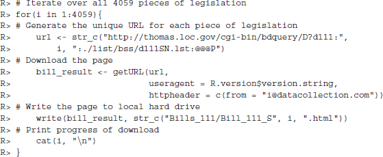
When you are finished downloading the data, inspect the source code of the first bill in a text editor of your choice. Notice that each senator—both sponsors and cosponsors—is provided with links which makes the task all the easier for us as we simply have to extract all the links in this specific format. Note the subtle difference in the link for the sponsor, Harry Reid,
/cgi-bin/bdquery/?&Db=d111&querybd=@FIELD(FLD003+@4
((@1(Sen+Reid++Harry))+00952))
and the—alphabetically speaking—first cosponsor, Mark Begich,
/cgi-bin/bdquery/?&Db=d111&querybd=@FIELD(FLD004+@4
((@1(Sen+Begich++Mark))+01898))
The former URL specifies that Harry Reid is in field 3 (FLD003) and Mark Begich in field 4 (FLD004). So, apparently, the Congress website internally differentiates between the sponsors and the cosponsors of a bill.
We can make use of this knowledge by writing two simple regular expressions to extract all the “field 3” links—there cannot be more than one in each site, as there is only one sponsor for each bill—and all the “field 4”links. To do so, we replace the senators’ names in the form of Sen+Reid++Harry with a sequence of alphabetic, plus, and period characters—[[:alpha:]+.]+?.4 Then, we precede all the characters with special meanings in regular expressions with two backslashes in order to have them interpreted literally.
R> sponsor_regex <- ”FLD003\+@4\(\(@1\([[:alpha:]+.]+”
R> cosponsor_regex <- ”FLD004\+@4\(\(@1\([[:alpha:]+.]+”
Now that we have our regular expressions set up, let us go for a test drive. We load the source code of the first senate bill into R and extract the link for the sponsor, as well as the links for the cosponsors.
R> html_source <- readLines(”Bills_111/Bill_111_1.html”)
R> sponsor <- str_extract(html_source, sponsor_regex)
R> (sponsor <- sponsor[!is.na(sponsor)])
[1] ”FLD003+@4((@1(Sen+Reid++Harry”
R> cosponsors <- unlist(str_extract_all(html_source, cosponsor_regex))
R> cosponsors[1:3]
[1] ”FLD004+@4((@1(Sen+Begich++Mark” ”FLD004+@4((@1(Sen+Bingaman++Jeff”
[3] ”FLD004+@4((@1(Sen+Boxer++Barbara”
R> length(cosponsors)
[1] 17
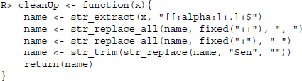
No problems here. Before moving on we write a small function that first extracts the senators’ names in the parentheses, drops the parentheses, replaces the + signs with commas and spaces, and, finally, takes out the leading Sen for convenience.
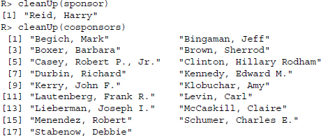
Applying the cleanUp() function to our previous results yields
Perfect. Now we want to run this code on our entire corpus. Before doing so, we would like to add a couple of fail safes in order to ensure that the code actually extracts what we want. In order to do so, we apply some knowledge on what the results should look like. The first thing we know is that there can only be one single sponsor for each bill. Accordingly, we check whether our code returns either no sponsor or more than one sponsor.
The second fail safe is a little more tricky. A bill can have one, many, or no cosponsors at all. Luckily, each site tells us the number of cosponsors it lists. We will read out this information and compare this number to the number of cosponsors we find. Specifically, we look for the elements COSPONSOR(S) and COSPONSOR(some_number) in the source code. If neither of these strings are present, we know something might be wrong. We also know that if the number of cosponsors in these strings does not match our findings, we better double-check our results. We store these errors in a list for later inspection. We cannot store the results in the proposed format from the beginning of this section, as we do not have a list of all senators that have at one point (co-)sponsored a bill. Hence, we input our results into a list of its own for the time being. The procedure is plotted in Figure 12.1.
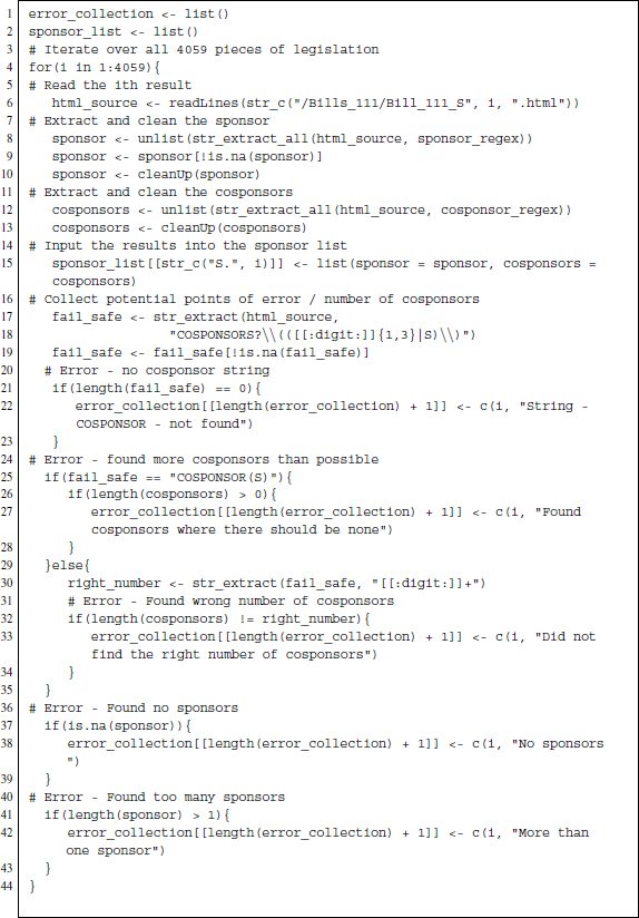
Figure 12.1 R procedure to collect list of bill sponsors
After assembling the list of sponsors and errors, we investigate the latter.
R> length(error_collection)
[1] 18
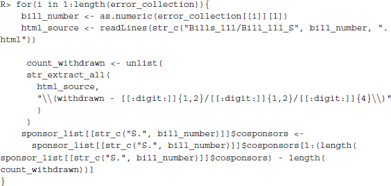
There are 18 errors in the error_collection list—all of them related to a discrepancy between the number of cosponsors recorded in the source code and the actual number collected by our code. A manual inspection of these cases reveals that all of them can be traced back to withdrawals of cosponsorship. We go back to them, load the source code again, count the number of withdrawals on a bill, and shorten the cosponsors list by the right amount—withdrawals are always last on the list.
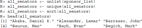
Now we have a complete list of all the senators that have either sponsored or cosponsored legislation in the 111th US Senate. We inspect the data by unlisting it, thus inputting it into a named character vector. Next, we deselect duplicates and print out the—alphabetically ordered—first five senators.
In the following step, we set up the matrix for the data as proposed in the beginning of the section. First, we create an empty matrix.
R> sponsor_matrix <- matrix(NA, nrow = 4059, ncol = length(all_senators))
R> colnames(sponsor_matrix) <- all_senators
R> rownames(sponsor_matrix) <- paste(”S.”, seq(1, 4059), sep =””)
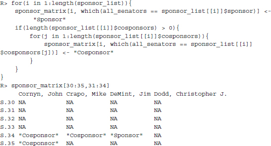
Finally, we iterate over our sponsor list to fill the correct cells.
12.2 Information on the senators
In this section, we want to collect some simple background information on the senators to use in our analysis. Specifically, we are interested in the party affiliation and the home state of the senators. We collect these data from the biographical archives of the Congress.5 Let us check out the source code of the website http://bioguide.congress.gov/biosearch/biosearch.asp. It mainly consists of an HTML form that can be accessed using the postForm() command. To request an answer from the form, we have to specify values for the different options the form has. There are several types of input an HTML form can take—two out of which are used in this case (see Section 9.1.5). There are three free inputs and three selections we can make that come with a list of prespecified options. Let us take a look at the options first by collecting them from the source code of the website. Again, in line with our rules of good practice, we start by storing the source code on our local hard drive before accessing it.
R> url <- ”http://bioguide.congress.gov/biosearch/biosearch.asp”
R> form_page <- getURL(url)
R> write(form_page, ”form_page.html”)
Accessing the form with regular expressions yields
R> form_page <- str_c(readLines(”form_page.html”), collapse = ””)
R> destination <- str_extract(form_page, ”<form.+?>”)
R> cat(destination)
<form method=”POST” action=”http://bioguide.congress.gov/biosearch/
biosearch1.asp”>

R> form <- str_extract(form_page, ”<form.+?</form>”)
R> cat(str_c(unlist(str_extract_all(form, ”<INPUT.+?>”)), collapse = ”
”))
<INPUT SIZE=30 NAME=”lastname” VALUE=””>
<INPUT SIZE=30 NAME=”firstname” VALUE=””>
<INPUT SIZE=4 NAME=”congress” VALUE=””>
<INPUT TYPE=submit VALUE=”Search”>
<INPUT TYPE=reset VALUE=”Clear”>

R> cat(str_c(unlist(str_extract_all(form, ”<SELECT.+?>”)), collapse = ”
”))
<SELECT NAME=”position” SIZE=1>
<SELECT NAME=”state” SIZE=1>
<SELECT NAME=”party” SIZE=1>
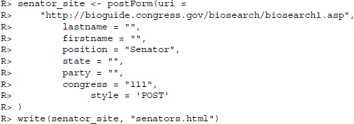
We see the options firstname, lastname, and congress as the free fields and position, state, and party as the fields with given options. We are interested in a list of all the senators in the 111th Senate, hence we specify these two values and leave the other fields open. The URL destination is specified in the form tag. For this request, we use the RCurl package which provides the useful postForm(). Note that the form expects application/x-www-form-urlencoded encoded content, so we add the argument style = ’POST’.
The response to this call holds the information we are looking for. We collect the information using the readHTMLTable() function.
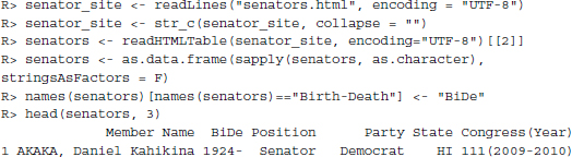
![]()
Here is where things become a little messy. We would like to match the senators along with their background information that we have collected in this section and stored in the object senators to the data were collected in the previous section. Recall that we created an object all_senators where we stored the names of all the senators that have at one point either sponsored or cosponsored a piece of legislation.
R> senators$match_names <- senators[,1]
R> senators$match_names <- tolower(senators$match_names)
R> senators$match_names <- str_extract(senators$match_names, ”[[:alpha:]]+”)
R> all_senators_dat <- data.frame(all_senators)
R> all_senators_dat$match_names <- str_extract(all_senators_dat$all_senators,
”[[:alpha:]]+”)
R> all_senators_dat$match_names <- tolower(all_senators_dat$match_names)
R> senators <- merge(all_senators_dat, senators, by = ”match_names”)
R> senators[,2] <- as.character(senators[,2])
R> senators[,3] <- as.character(senators[,3])
R> senators[,2] <- tolower(senators[,2])
R> senators[,3] <- tolower(senators[,3])
We match by last names but unfortunately, there are no less than eight senators in the 111th Senate of identical last names. We treat these duplicates by matching them by first name.
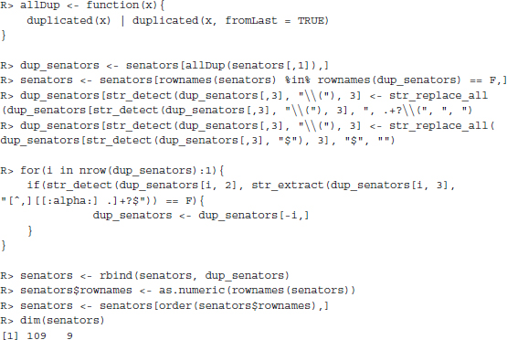
Finally, we replace the column names in the sponsor matrix with these shortened identifiers.
R> colnames(sponsor_matrix) <- senators$all_senators
Now that we have collected information on the bills and the Senators, we will briefly introduce how the data could be applied in a network analysis. If you simply care about data collection, but not about network analysis, you can skip the following section without much loss.
12.3 Analyzing the network structure
In order to analyze our data using network analysis techniques, we need to rearrange it to conform to a format that the network packages understand. Two common ways to arrange the data are an edge list or an adjacency list. In the former variant, we generate a two-column matrix where each edge between two nodes or vertices is represented by naming the two vertices an edge connects. In an adjacency list, on the other hand, we store the network data in a nodes-by-nodes matrix, setting a cell to the number of connections between two nodes. While an adjacency list would be computationally more efficient since our data have multiple edges, that is, any two Senators might have been cosponsors on numerous bills—we, nevertheless, create an edge list for coding convenience.
In the network analysis, we assume that there is an undirected relationship between each of the signatories of a particular bill, regardless of whether a senator is a sponsor or a cosponsor. For example, assume there is a bill with one sponsor and three cosponsors. What we would like to have is each possible dyadic relationship between these four actors (see Table 12.2).
Table 12.2 Dyadic relationships between four hypothetical actors
| Node 1 | Node 2 |
| Senator A | Senator B |
| Senator A | Senator C |
| Senator A | Senator D |
| Senator B | Senator C |
| Senator B | Senator D |
| Senator C | Senator D |
The table displays an example of the resulting graph edge list. Specifically, it displays all six possible dyadic combinations with four input senators.
There is a simple function available in R—combn()—which we will use to find all of these dyadic relationships. We create an empty edge list matrix with two columns and iterate over the matrix of sponsors and cosponsors from Section 12.1. In each iteration we take all the non-empty elements from a row, find all possible combinations, and attach the resulting two-column matrix to our final matrix.
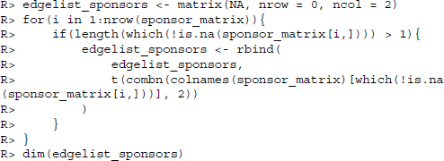
Performing this operation yields a matrix with a little over 180,000 edges, that is, there are approximately 180,000 unique binary connections between the 109 senators in our dataset. Now we would like to convert these data into the format used in the igraph package which offers a range of tools and some decent plotting facilities.6 Specifying that we are dealing with an undirected network, the command is
R> sponsor_network <- graph.edgelist(edgelist_sponsors, directed = F)
12.3.1 Descriptive statistics
Before moving on to some real network analysis, let us inspect the data we have gathered. Let us first look at who sponsors/cosponsors most/least. To do so, we simply create a two-row matrix where we collect the individual counts of being a sponsor and cosponsor for each senator.
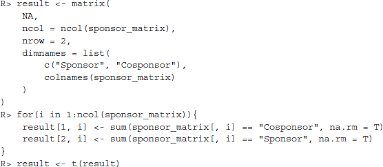
Table 12.3 displays a subset of the results of this analysis. We see that Democrats have been the most active sponsors in the 111th Senate, although to be fair they have a slightly better chance of being at the top of the table as our table holds 65 Democratic Senators compared to 43 Republicans and 2 independents.7
Table 12.3 The five top and bottom sponsors
| Senator | Sponsor | Cosponsor | |
| Brown, Sherrod | (D-OH) | 377 | 107 |
| Gillibrand, Kirsten E. | (D-NY) | 357 | 74 |
| Casey, Robert P., Jr. | (D-PA) | 355 | 99 |
| Schumer, Charles E. | (D-NY) | 333 | 133 |
| Kerry, John F. | (D-MA) | 321 | 96 |
| Coons, Christopher A. | (D-DE) | 11 | 0 |
| Goodwin, Carte Patrick | (D-WV) | 5 | 1 |
| Salazar, Ken | (D-CO) | 4 | 6 |
| Kirk, Mark Steven | (R-IL) | 2 | 1 |
| Manchin, Joe, III | (D-WV) | 1 | 0 |
The tables displays the five senators which have sponsored most and least legislation.
In the next descriptive statistic we care to find out which senators have the strongest binary connection with each other. The simplest way to do this is to convert our data to an adjacency matrix where the greatest dyadic relationships are summed in a vertex by vertex table. We get this table by making use of the export utility in the igraph package.
R> adj_sponsor <- get.adjacency(sponsor_network)
Naturally, the resulting matrix is symmetric, as we have no directed relationships. Therefore, we discard the lower triangle of the matrix before calculating the greatest binary relationships.
R> adj_sponsor[lower.tri(adj_sponsor)] <- 0
Finally, we extract the dyads with the strongest binary relationships. The results are displayed in Table 12.4.
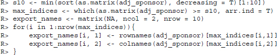
Table 12.4 The senators with the strongest binary connection
| Senator 1 | Senator 2 | |||
| 1 | Brown, Sherrod | (D-OH) | Casey, Robert P., Jr. | (D-PA) |
| 2 | Brown, Sherrod | (D-OH) | Durbin, Richard | (D-IL) |
| 3 | Lautenberg, Frank R. | (D-NJ) | Menendez, Robert | (D-NJ) |
| 4 | Brown, Sherrod | (D-OH) | Schumer, Charles E. | (D-NY) |
| 5 | Durbin, Richard | (D-IL) | Schumer, Charles E. | (D-NY) |
| 6 | Kerry, John F. | (D-MA) | Schumer, Charles E. | (D-NY) |
| 7 | Menendez, Robert | (D-NJ) | Schumer, Charles E. | (D-NY) |
| 8 | Brown, Sherrod | (D-OH) | Stabenow, Debbie | (D-MI) |
| 9 | Casey, Robert P., Jr. | (D-PA) | Specter, Arlen | (D-PA) |
| 10 | Schumer, Charles E. | (D-NY) | Gillibrand, Kirsten E. | (D-NY) |
It is fairly obvious that the most active sponsors and co-sponsors would rank high in this table as they have a greater probability to have a strong connection to any given other senator.
12.3.2 Network analysis
Let us begin the analysis by visually inspecting the resulting network. As a first step we would like to simplify the network by turning multiple edges into unique edges and keeping multiples as weights. This is accomplished using the simplify() function from the igraph package.
R> E(sponsor_network)$weight <- 1
R> sponsor_network_weighted <- simplify(sponsor_network)
R> sponsor_network_weighted
R> head(E(sponsor_network_weighted)$weight)
After applying this simplification, our network still has more than 5000 unique edges—much more than can be visually inspected. Hence, for the purpose of plotting we only display those edges that conform to a cutoff point that we define as follows: Only display those edges that have an edge weight greater than the mean edge weight plus one standard deviation. This operation yields the graph in Figure 12.2.
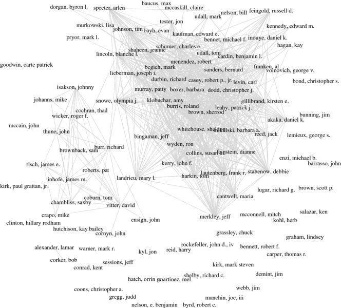
Figure 12.2 Cosponsorship network of senators
We can clearly distinguish the two major parties in this graph as dense blocks. Interestingly, there a numerous senators which are completely disconnected to the graph after applying the thinning operation. If we go into a little more detail, there are a number of remarkable findings which confirm the intuition that cosponsorships are indeed a viable proxy for intra-parliamentary collaboration. Consider Olympia Snowe from Maine at the center of the graph. While still in office she was widely regarded as one of the most moderate Republicans in the Senate, which is nicely reflected in her being one of the only bridging nodes in the graph. In fact, this finding is even more remarkable if one considers that she has numerous strong connections to the Democratic party while her only strong connection to the Republican party is Senator Richard Burr from North Carolina. Time and again, she was considered one of the likely candidates for a party switch which finds a clear visual expression in our analysis. By a similar token, consider Mary Landrieu from Louisiana. She is frequently labeled as one of the most conservative Democrats in the Democratic party and indeed she also takes up a central location in our graph.
Consider now a true network metric—the betweenness centrality. This measure describes how central any given node is in the overall network, which is typically taken as an indicator of influence in a network. It is defined as the shortest path from all nodes to all other passing through a node. The higher the score, the more central the actor's position in the network. Table 12.5 provides an overview of the five most central actors, ranked by betweenness. We find that among the five most central actors there are no less than two who went on to serve as secretaries in the Obama Administration.
Table 12.5 The five most central actors
| Senator | Betweenness | |
| Goodwin, Carte Patrick | (D-WV) | 2217 |
| Salazar, Ken | (D-CO) | 2058 |
| Clinton, Hillary Rodham | (D-NY) | 1062 |
| Kirk, Paul Grattan, Jr. | (D-MA) | 618 |
| Coons, Christopher A. | (D-DE) | 245 |
The tables displays the five most central senators, based on their betweenness scores.
12.4 Conclusion
Scholars of parliamentary politics have recently begun employing large-scale data sources in order to come to terms with long-standing research questions. Among the issues that have come under scrutiny are patterns of intra-parliamentary collaboration. Using cosponsorships as proxies for cooperation, a number of scholars have investigated these manifested networks. This chapter has demonstrated how to assemble the necessary data to perform analyses of the like that have been proposed in the literature. We have shown that the data informing these analyses are vast. We were able to collect well over 100,000 unique dyadic relations in a single senatorial term. In terms of substance, we have not delved deeply into the data but, using very simple indicators, we were able to show that the data exhibit strong face validity. First, moderate members of either party have been shown to take up plausible center points in the network. Second, senators who are widely perceived as influential members of the body could indeed be shown to take up more central locations in the network.
As in many of the examples throughout this volume there are clear advantages of automatically collecting the data as proposed here. We have only assembled a single senatorial term, but the resulting dataset is immense. Never before have datasets of such size been in the reach of single researchers interested in a particular topic. What is more, not only is the data vast, it is also freely available to anyone who brings the right techniques to the table. It can quickly be updated so that results are informed by current events. And finally, using automatic data assembly one avoids the risk of coding errors in the data which are to be expected when hand-coding a dataset of this size. We encourage you to assemble the data yourselves, toy around with it and investigate the ad hoc claims in this exploratory chapter to present some new insights on patterns of parliamentary collaboration.