
13
Parsing information from semistructured documents
We have learned how to handle and extract information from well-defined data structures like XML or JSON. There are standardized methods for translating these formats into R data structures. Content on the Web is highly heterogeneous, however. We are occasionally confronted with data which are structured but in a format for which no parser exists.
In this chapter, we demonstrate how to construct a parser that is able to transform pure character data into R data structures. As an example we identified climate data that are offered by the Natural Resources Conservation Service at the United States Department of Agriculture.1 We focus on a set of text files that can be downloaded from an FTP server.2 While the download procedure is simple, the files cannot be put into an R data structure directly. An excerpt from one of these files is shown in Figure 13.1. The displayed data are structured in a way which is human-readable but not (yet) understandable by a computer program. The main goal is to describe the structure in a way that a computer can handle them.
Over the course of the case study we make use of RCurl to list files on and retrieve them from FTP servers and draw on R’s text manipulation capabilities to build a parser for the data files. Regular expressions are a crucial tool to solve this task.
13.1 Downloading data from the FTP server
First, we load RCurl and stringr. As we have learned, RCurl provides functionality to access data from FTP servers (see Section 9.1.2) and stringr offers consistent functions for string processing with R.
R> library(RCurl)
R> library(stringr)
A folder called Data is created to store the retrieved data files. The data we are looking for are stored on an FTP server and accessible at a single url which we store in ftp. Note that this is only a rather tiny subdirectory—the server provides tons of additional climate data.
R> dir.create(”Data”)
R> ftp <- ”ftp://ftp.wcc.nrcs.usda.gov/data/climate/table/temperature/history/california/”
The RCurl function getURL() with option dirlistonly set to TRUE asks the FTP server to return a list of files instead of downloading a file.
R> filelist <- getURL(ftp, dirlistonly = TRUE)
This is the returned list of files:
R> str_sub(filelist, 1, 119)
[1] ”19l03s_tavg.txt
19l03s_tmax.txt
19l03s_tmin.txt
19l05s_tavg.txt
19l05s_tmax.txt
19l05s_tmin.txt
19l06s_tavg.txt
”
In order to identify the file names, we split the text by carriage returns ( ) and new line characters ( ) and keep only those vector items that are not empty.
R> filelist <- unlist(str_split(filelist, ”
”))
R> filelist <- filelist[!filelist == ””]
R> filelist[1:3]
[1] ”19l03s_tavg.txt” ”19l03s_tmax.txt” ”19l03s_tmin.txt”
A comparison with the files at the FTP interface reveals that we have succeeded in identifying the file names. As we are not interested in minimum or maximum temperatures for now, we use str_detect() to only keep files containing tavg in their file name.
R> filesavg <- str_detect(filelist, ”tavg”)
R> filesavg <- filelist[filesavg]
R> filesavg[1:3]
[1] ”19l03s_tavg.txt” ”19l05s_tavg.txt” ”19l06s_tavg.txt”
To download the files we have to construct the full URLs that point to their location on the server. We concatenate the base URL and the created vector of file names and retrieve a vector of full URLs.
R> urlsavg <- str_c(ftp, filesavg)
R> length(urlsavg)
[1] 32
R> urlsavg[1]
[1] ”ftp://ftp.wcc.nrcs.usda.gov/data/climate/table/temperature/history/california/19l03s_tavg.txt”
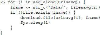
Having built the URLs for the 32 files, we can now loop over each URL and save the text files to our local folder. We introduce a check if the file has previously been downloaded using the file.exists() function and stop for 1 second after each server request. The files themselves are downloaded with download.file() and stored in the Data folder.
A brief inspection of the local folder reveals that we succeeded in downloading all 32 files.
R> length(list.files(”Data”))
[1] 32
R> list.files(”Data”)[1:3]
[1] ”19l03s_tavg.txt” ”19l05s_tavg.txt” ”19l06s_tavg.txt”
13.2 Parsing semistructured text data
Now that we have downloaded all the files we want, we can have a look at their content. Let us reconsider Figure 13.1 which provides an example of the content of the files. Because they are quite long—more than 1,000 lines, we only present a small sample.
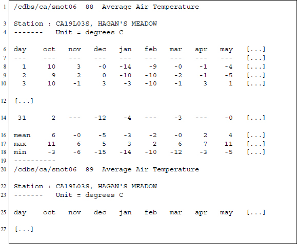
Figure 13.1 Excerpt from a text file on temperature data from Californian weather stations, accessible at ftp://ftp.wcc.nrcs.usda.gov/data/climate/table/temperature/history/california/
Each file provides daily temperature data for one station in California ranging from 1987 up to 2013. We see from the sample that for each year there is a separate section ending with ----------. The first line tells us something about the source of the data (/cdbs/ca/snot06), followed by the year expressed as two digits (88) and the type of data that is presented (Average Air Temperature). Next is a line identifying the station at which the temperatures were measured (Station : CA19L03S, HAGAN'S MEADOW), followed by a line expressing the unit in which the measurements are stored (Unit = degrees C).
After the header sections comes the actual data presented in a table, where columns indicate months and rows refer to days. If days do not exist within a month—like November 31—we find three dashes in the cell: ----. Beneath the daily temperature we also find a section with monthly data that provides mean, maximum, and minimum temperatures for each month. If the temperature data tables would be the only information provided and the only information we were interested in, our task would be easy because R can handle tables written in fixed-width format: read.fwf() reads such data and transforms them automatically into data frames. The problem is that we do not want to loose the information from the header section because it tells us to which year and which station the temperatures belong to.
When we proceed, it is important to think about which information should be extracted and what the data should look like at the end. In the end a long table with daily temperatures and variables for the day, month, and year when the temperatures were measured as well as the station's id and its name should do. The resulting data structure should look like the one depicted in Table 13.1.
Table 13.1 Desired data structure after parsing
| day | month | year | id | name |
| 1 | 1 | 1982 | XYZ001784 | Deepwood |
| 2 | 1 | 1982 | XYZ001784 | Deepwood |
| ... | ... | ... | ... | ... |
| 31 | 12 | 1984 | XYZ001786 | Highwood |
| 1 | 1 | 1985 | XYZ001786 | Highwood |
| … | … | … | … | … |
| 3 | 3 | 2003 | XYZ001800 | Northwood |
| 4 | 3 | 2003 | XYZ001800 | Northwood |
Because information is separated into sections, we should first split the text to turn them into separate vectors. To do this, we first read in all the text files via readLines() and input the resulting lines into a vector.
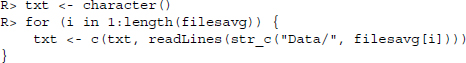
In a next step, we collapse the whole vector into one single line, where the newline character ( ) marks the end of the original lines. We split that single line at each occurrence of ---------- , marking the end of a section.
R> txt <- str_c(txt, collapse = ”
”)
R> txtparts <- unlist(str_split(txt, ”----------
”))
The resulting vector contains one section per line.
R> str_sub(txtparts[28:30], 1, 134)
[1] ”
***This data is provisional and subject to change.
/cdbs/ca/snot06
84 Average Air Temperature

Station : CA19L05S, BLUE LAKES
---–”
[2] ”/cdbs/ca/snot06 85 Average Air Temperature

Station : CA19L05S,
BLUE LAKES
------- Unit = degrees C

day oct nov dec jan ”
[3] ”/cdbs/ca/snot06 86 Average Air Temperature

Station : CA19L05S,
BLUE LAKES
------- Unit = degrees C

day oct nov dec jan ”
In a text editor, this would look as follows:
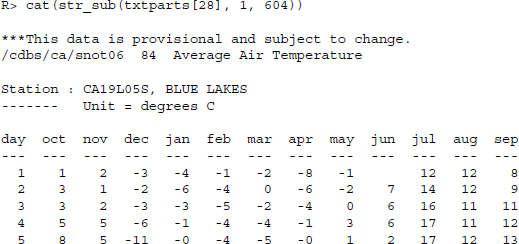
Now we need to do some cleansing to get rid of the statement saying that the data are provisional and delete all lines of the vector that are empty.
R> txtparts <- str_replace(txtparts,”
\*\*\*This data is
provisional and subject to change.”, ””)
R> txtparts <- str_replace(txtparts,”⁁
”, ””)
R> txtparts <- txtparts[txtparts!=””]
Having inserted each section into a separate line, we can now build functions for extracting information that can be applied to each line, as each line contains the same kind of information structured in the same way. We start by extracting the year in which the temperature was measured. To do this, we build a regular expression that looks for a character sequence that starts with two digits, followed by two white spaces, followed by Average Air Temperature: ”[[:digit:]]{2} Average Air Temperature”. We then extract the digits from that substring and append the two digits in a third step to a four digit year.
R> year <- str_extract(txtparts, ”[[:digit:]]{2} Average Air Temperature”)
R> year[1:4]
[1] ”87 Average Air Temperature” ”88 Average Air Temperature”
[3] ”89 Average Air Temperature” ”90 Average Air Temperature”
R> year <- str_extract(year, ”[[:digit:]]{2}”)
R> year <- ifelse(year < 20, str_c(20, year), str_c(19, year))
R> year <- as.numeric(year)
R> year[5:15]
[1] 1991 1992 1993 1994 1995 1996 1997 1998 1999 2000 2001
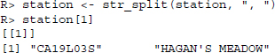
We also gather the stations’ names as well as the identification. For this we first extract the line where the station information is saved.
R> station <- str_extract(txtparts, ”Station : .+?
”)
R> station[1:2]
[1] ”Station : CA19L03S, HAGAN'S MEADOW
”
[2] ”Station : CA19L03S, HAGAN'S MEADOW
”
We delete those parts that are of no interest to us—Station : and …
R> station <- str_replace_all(station, ”(Station : )|(
)”, ””)
R> station[1:2]
[1] ”CA19L03S, HAGAN'S MEADOW” ”CA19L03S, HAGAN'S MEADOW”
…and split the remaining text into one part that captures the id and one that contains the name of the station.
The splitting of the text results in a list where each list item contains two strings. The first string of each list item is the id while the second captures the name. To extract the first and second string from each list item, we apply the [ operator to each item.
R> id <- sapply(station, ”[”, 1)
R> name <- sapply(station, ”[”, 2)
R> id[1:3]
[1] ”CA19L03S” ”CA19L03S” ”CA19L03S”

R> name[1:3]
[1] ”HAGAN'S MEADOW” ”HAGAN'S MEADOW” ”HAGAN'S MEADOW”
Now we can turn our attention to extracting the daily temperatures. The temperatures form a table in fixed-width format that can be read and transformed by read.fwf(). In the fixed width format each entry of a column has the same width of characters and lines are separated by newline characters or carriage returns or a combination of both. What we have to do is to extract that part of each section that forms the fixed width table and apply read.fwf() to it.
Our first task is to extract the part that contains the temperature table. To do so, we use a regular expression that extracts day and everything after.
R> temperatures <- str_extract(txtparts, ”day.*”)
Further below, we will write the next steps into a function that we can apply to each of the temperature tables, but for now we go through the necessary steps using only one temperature table to develop all the intermediate steps.
As read.fwf() expects a filename as input, we first have to write our temperature table into a temporary file using the tempfile() function.
R> tf <- tempfile()
R> writeLines(temperatures[5], tf)
We can then use read.fwf() to read the content back in. The width option tells the function the column width in characters.
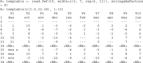
There are several lines in the data that do not contain the data we need. Therefore, we only keep lines 3–33 and also discard the first column.
R> temptable <- temptable[3:33, -1]
In the next step, we transform the table into a vector. Using as.numeric() and unlist() all numbers will be transferred to type numeric, while all cells containing only white spaces or --- are set to NA.
R> temptable <- as.numeric(unlist(temptable))
Having discarded the table structure and kept only the temperatures, we now have to reconstruct the days and months belonging to the temperatures. Fortunately, unlist() always decomposes data frames in the same way. It starts with all rows of the first column and appends the values of the following columns one by one. As we know that in the temperature tables rows referred to days and columns to months, we can simply repeat the day sequence 1–31 twelve times to get the days right. Similarly, we have to repeat each month 31 times. Note that the order of the months differs from the usual 1–12 because the tables start with October.
R> day <- rep(1:31, 12)
R> month <- rep(c(10:12, 1:9), each = 31)
Now we combine the information on the year of measurement and the weather station with the temperatures and get the data for 1 year.
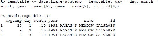
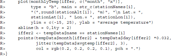
To get all the data, we have to repeat the procedure for all files. For convenience we have constructed a parsing function that takes a file name as argument and returns a ready-to-use data frame. The code is shown in Figure 13.2. Applying the function yields:
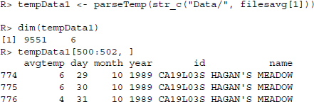
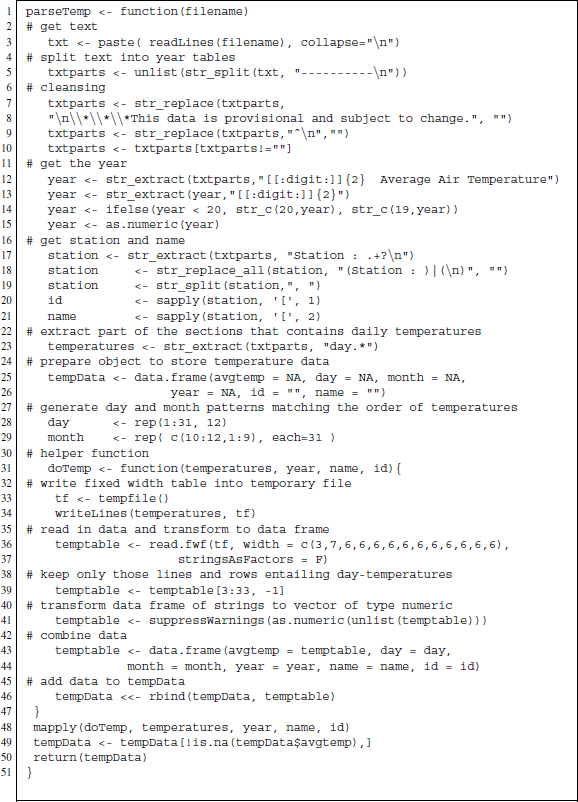
Figure 13.2 R-based parsing function for temperature text files
This looks like a successful parsing result. Furthermore, to conveniently parse all files at once, we can create a wrapper function that takes a vector of file names as argument and returns a combined data frame.
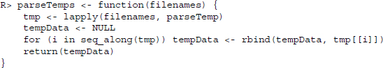
Finally we apply the wrapper to all files in our folder.
R> tempData <- parseTemps(str_c(”Data/”, filesavg))

R> dim(tempData)
[1] 252463 6
13.3 Visualizing station and temperature data
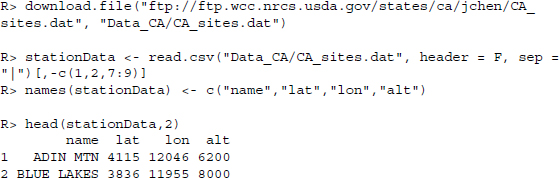
We conclude the study with some examples of what to do with the data. First it would be nice to know the location of the weather stations. We already know that they are in California, but want to be a little more specific. Browsing the FTP server we find a file that contains data on the stations—station names, their position expressed as latitudes and longitudes as well as their altitude. We download the file and read it in via read.csv() .
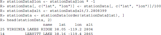
With regards to the map which we are going to use, we have to rescale the coordinates. First, we multiply all longitudes by −1 to get general longitudes and divide all coordinates by 100. Altitudes are measured in foot, so we transform them to meters.
Now we plot the stations’ locations on a map. In R, there are several packages suitable for plotting maps (see also Chapter 15). We choose RgoogleMaps which enables us to use services provided by Google and OpenStreetMap to download maps that we can use for plotting. We download map data from Open Street Maps using the GetMap.OSM() function. With this function we define a bounding box of coordinates and a scale factor. The map data are saved on disk in PNG format as map.png and in an R object called map for later use:
R> map <- GetMap.OSM(latR = c(37.5, 42), lonR = c(-125, -115), scale =
5000000, destfile = ”map.png”, GRAYSCALE = TRUE, NEWMAP = TRUE)
Now we can use PlotOnStaticMap() to print the weather stations’ locations on the map we previously downloaded. The result is presented in Figure 13.3.
R> png(”stationmap.png”, width = dim(readPNG(”map.png”))[2], height =
dim(readPNG(”map.png”))[1])

R> PlotOnStaticMap(map, lat = stationData$lat, lon = stationData$lon,
cex = 2, pch = 19, col = rgb(0, 0, 0, 0.5), add = FALSE)
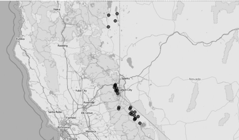
Figure 13.3 Weather station locations on an OpenStreetMaps map
Finally, we visualize the temperature data. Let us look at the average temperatures per month for six out of 27 stations. First, we aggregate the temperatures per month and station using the aggregate() function.
R> monthlyTemp <- aggregate(x = tempData$avgtemp, by = list(name =
tempData$name, month = tempData$month), FUN = mean)
The stations we choose are representative of all others—we select three stations which are placed north of the the mean latitude and three south of it. Furthermore, within each group stations should differ regarding their altitude and should roughly match one station of the other group. Looking through the candidates we find the following stations to be fitting and extract their coordinates and their altitude:
R> stationNames <- c(”ADIN MTN”, ”INDEPENDENCE CAMP”, ”SQUAW VALLEY
G.C.”, ”SPRATT CREEK”, ”LEAVITT MEADOWS”,”POISON FLAT”)

R> stationAlt <- stationData[match(stationNames, stationData$name), ]$alt
R> stationLat <- stationData[match(stationNames, stationData$name), ]$lat
R> stationLon <- stationData[match(stationNames, stationData$name), ]$lon
Then, we prepare a plotting function to use on all plots. The function first defines an object called iffer that serves to select only those monthly temperatures that belong to the station to be plotted. The overall average per station and month is plotted with adequate title and axis labels. We add a horizontal line to mark 0°C . To get an idea of the variation of temperature measurements over time, we add the actual temperature measurements in a last step as small gray dots.
![]()
Having defined the plot function, we loop through the selection of stations.
R> par(mfrow = c(2, 3))
R> for (i in seq_along(stationNames)) plotTemps(i)
Figure 13.4 presents the average monthly temperatures. Little surprisingly, the higher the altitude of the station and the more north the station is located, the lower the average temperatures.
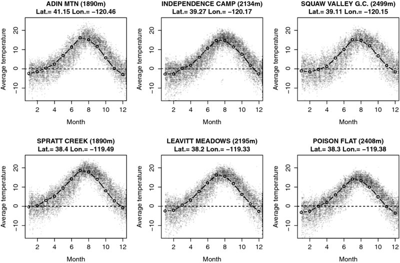
Figure 13.4 Overall monthly temperature means for selected weather stations. Lines present average monthly temperatures in degree Celsius for all years in the dataset. Small gray dots are daily temperatures for all years within the dataset.