
10
Statistical text processing
Any quantitative research project that hopes to make use of statistical analyses needs to collect structured information. As we have demonstrated in countless examples up to this point, the Web is an invaluable source of structured data that is ready for analysis upon collection. Unfortunately, in terms of quantity such structured information is far outweighed by unstructured content. The Internet is predominantly a vast collection of more or less unclassified text.
Consequently, the advent of the widespread use of the Internet has seen a contemporaneous interest in natural language processing—the automated processing of human language. This is by no means coincidental. Never before have such massive amounts of machine-readable text been available. In order to access such data, numerous techniques have been devised to assign systematic meaning to unstructured text. This chapters seeks to elaborate several of the available techniques to make use of unclassified data.
In a first step, the next section presents a small running example that is used throughout the chapter. Subsequently, Section 10.2 elaborates how to perform large-scale text operations in R. Textual data can quickly become taxing on resources. While this is a more general concern when dealing with textual data, it is particularly relevant in R, which was not designed to deal with large-scale text analysis. We will introduce the tm package that allows the organization and preparation of text and also provides the infrastructure for the analytical packages that we will use throughout the remainder of the chapter (Feinerer 2008; Feinerer et al. 2008).
In terms of the techniques that are presented in order to make sense of unstructured text data, we start out by presenting supervised methods in Section 10.3. This broad class of techniques allows the categorization of text based on similarities to pre-classified text. Simply put, supervised methods allow users to label texts based on how much they resemble a hand-coded training set. The classic example in this area deals with the organization of text into topical categories. Say we have 1000 texts of varied content. Imagine further that half of the texts have been assigned a label of their topical emphasis. Using supervised methods we can estimate the content of the unlabeled half.1 Several supervised methods have been made available in R. This chapter introduces the RTextTools package which provides a wrapper to a number of the available packages. This allows a convenient access to several classifiers from within a single function call (Jurka et al. 2013).
A second approach to classifying text is presented in Section 10.4—unsupervised classifiers. In contrast to supervised learning algorithms that rely on similarities between pre-classified and unlabeled text, unsupervised classifiers estimate the categories along with the membership of texts in the different categories. The major advantage of techniques in this group is the possibility of circumventing the cumbersome hand-coding of training data. This advantage comes at the price of having to interpret the content of the estimated categories a posteriori.
As a word of caution we would like to point out that this chapter can only serve as a cursory introduction to the topics in question. We investigate some of the most important topics and packages that are available in R. It should be emphasized, however, that in many instances we cannot do full justice to the details of the topics that are being covered. You should be aware that if you care to deal with these types of models, there is a lot more out there that might serve your purposes better than what is being presented in this chapter. We provide some guidance for further readings in the last section of the chapter.
10.1 The running example: Classifying press releases of the British government
Before turning to the statistical processing of text, let us collect some sample text data that will serve as a running example throughout this chapter. For the running example, we want all the data to be labeled such that we have a benchmark for the accuracy of our classifiers. We have selected press releases from the UK government as our test case. The data can be accessed at https://www.gov.uk/government/announcements. Opening the website in a browser, you see several selection options at the left side of the screen. We want to restrict our analysis to press releases in all topics, from all departments, in all locations that were published before July 2010. At the time of writing this yields 747 results that conform to the request. The results page presents the title of the press release, the date of publication, an acronym signaling the publishing department, as well as the type of publication. For the statistical analysis in the subsequent chapters, we will consider the publishing agency as a marker of the press releases’ content.
Notice how the URL of the page changes when you make the selections.
You can clearly see how the selections we make become integrated into the URL. As the data are not too large to be stored locally, we will, in accordance with our rules of good practice in web scraping, start by downloading all 747 results onto our hard drive before collecting the text data in a tm corpus in a subsequent step. Check out the source code of the page. You will find the first results toward the end of the page. However, not all 747 results are contained in the source code. To collect them, we have to use the link that is contained at the bottom of the press releases. It reads
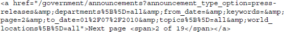
To assemble the links to all press releases, we collect the publication links in one page, select the link to the next page, and repeat the process until we have all the relevant links. This is achieved with the following short code snippet. First, we load the necessary scraping packages.
R> library(RCurl)
R> library(XML)
R> library(stringr)
We move on to download all the results. Notice that because the content is stored on an HTTPS server, we specify the location of our CA signatures (see Section 9.1.7 for details).
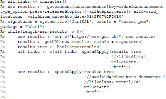
We are left with a vector of length 747 but possibly some changes have been made since this book was published. Each entry contains the link to one press release. To be sure that your results are identical to ours, check the first item in your vector. It should read as follows
R> all_links[1]
[1] ”/government/news/bianca-jagger-how-to-move-beyond-oil”
R> length(all_links)
[1] 747
To download all press releases, we iterate over our results vector.
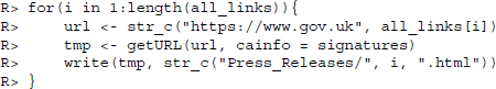
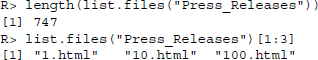
If everything was proceeded correctly, you should find the folder Press_Releases in your working directory which contains all press releases as HTML files.
10.2 Processing textual data
The widespread application of statistical text analysis is a fairly recent phenomenon. It coincides with the almost universal storage of text in digital formats. Such massive amounts of machine-readable text created the need to come up with methods to automate the processing of content. A number of techniques in the tradition of performing statistical text analysis have been implemented in R. Concurrently, infrastructures had to be implemented in order to handle large collections of digital text. The current standard for statistical text analysis in R is the tm package. It provides facilities to manage text collections and to perform the most common data preparation operations prior to statistical text analysis.
10.2.1 Large-scale text operations—The tm package
Let us load all press releases that we have collected in the previous section into R and store them in a tm corpus.2 Ordinarily, this could be accomplished by calling the relevant functions on the entire directory in which we stored the press releases. In this case, however, the press releases are still in the HTML format. Thus, before inputting them into a corpus, we want to strip out all the tags and text that is not specific to the press release.
Let us consider the first press release as an example. Open the press release in a browser of your choice. The press release starts with the words “Bianca Jagger, Chair of the Bianca Jagger Human Rights Foundation and a Council of Europe Goodwill Ambassador, has called for a “Copernican revolution” in moving beyond carbon to a decentralized, sustainable energy system.” There is more layout information in the document. In a real research project, one might want to consider stripping out the additional noise. In addition to the text of the press release we find the publishing organization and the date of publication toward the top of the page. We extract the first two bits of information and store them along with the press release as meta information. Let us investigate the source code of the press release. We find that the press release is stored after the tag <div class=”block-4”>. Thus, we get the release by calling
R> tmp <- readLines(”Press_Releases/1.html”)
R> tmp <- str_c(tmp, collapse = ””)
R> tmp <- htmlParse(tmp)
R> release <- xpathSApply(tmp, ”//div[@class=’block-4’]”, xmlValue)
The extracted release is not evenly formatted since we discarded all the tags. However, as we will drop the sequence of the words later on, this is of no concern. Also, while we might like to drop several bits of text like (opens in new window), this should not influence our estimation procedures.3 Before iterating over our entire corpus of results, we write two queries to extract the meta information. The information on the publishing organization is stored under <span class=”organisation lead”, the information on the publishing date under <dd class=”change-notes”>.
R> organisation <- xpathSApply(tmp, ”//span[@class=’organisation lead’]”, xmlValue)
R> organisation
[1] ”Foreign & Commonwealth Office”
R> publication <- xpathSApply(tmp, ”//dd[@class=’change-notes’]”, xmlValue)
R> publication
[1] ”Published 1 July 2010”
Now that we have all the necessary elements set up, we create a loop that performs the operations on all press releases and stores the resulting information in a corpus. Such a corpus is the central element for text operations in the tm package. It is created by calling the Corpus() function on the first press release we just assembled. The text release is wrapped in a VectorSource() function call. This specifies that the corpus is created from text which is stored in a character vector.4
R> library(tm)
R> release_corpus <- Corpus(VectorSource(release))
The corpus can be accessed just like any ordinary list by specifying the name of the object (release_corpus) and adding the subscript of the element that we are interested in, enclosed by two square brackets. So far, we have only stored one element in our corpus that we can call using release_corpus[[1]]. To add the two pieces of meta information to the text, we use the meta() function. The variable specifies the document that we want the meta information to be assigned to and the second variable specifies the tag name of the meta information, in our case we select organisation and publication. Note that we select the first organization for the meta information. Several press releases have more than one organizational affiliation. For convenience, we simply choose the first one. Again, this creates a little bit of imprecision in our data that should not throw off the classifiers terribly.
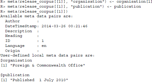
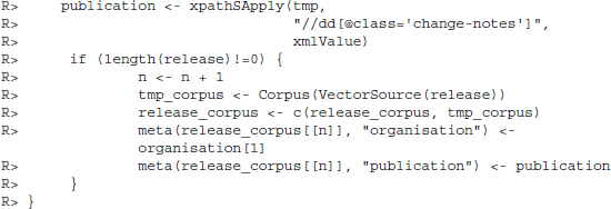
The meta information of any document can be accessed using the same function. Several meta information tags are predefined, such as Author and Language. Some are filled automatically upon creation of the entry. At the bottom of the meta information we see the two elements that we have created—the date of publication and the organization that has published the press release. In the next step, we perform the operations that we have introduced above for all the documents that we downloaded. We collect the text of the press release and the two pieces of meta information and add them our corpus using simple concatenation (c()). A potential problem of the automated document import is that the XPath queries may fail on press releases which have a different layout. Usually, this should not be the case. Nevertheless, if it did happen, our temporary corpus object tmp_corpus code would not be created and the loop would fail. We therefore specify a condition to conduct the corpus creation only if the release object exists, that is, has a length greater 0.5

A look at the full corpus reveals that all but one document have been added to the corpus object.
R> release_corpus
A corpus with 746 text documents
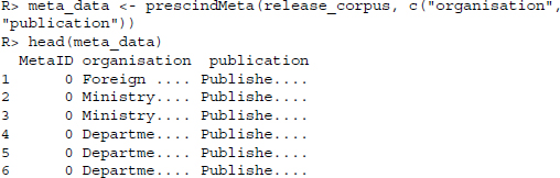
Recall that meta information is internally linked to the document. In many cases we are interested in a tabular form of the meta data to perform further analyses. Such a table can be collected using the prescindMeta() function. It allows selecting pieces of meta information from the individual documents to input them into a common data.frame.
Let us inspect the meta data for a moment. As a simple summary statistic we call a count of the different publishing organizations. We find that the publishing behavior of the various governmental departments is fairly diverse. Assuming that the website of the UK government truly collects all the press releases from all governmental departments we find that while two departments have released over 100 announcements, others have published less than a dozen.
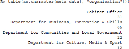

As we will elaborate in greater detail in the upcoming sections, we need a certain level of coverage in each of the categories that we would like the classifiers to pick up. Thus, we discard all press releases from departments that have released 20 press statements or less. There are eight departments that have published more than 20 press releases for the period that is covered by the website up to July 2010. We select them to remain in the corpus. In addition to the rare categories, we exclude the cabinet office and the prime minister's office. These bodies are potentially more difficult to classify as they are not bound to a particular policy area. We perform the exclusion of documents using the sFilter() function. This function takes the corpus in question as the first argument and one or more value pairs of the form ”tag == ’value”’. Recall that the pipe operator (|) is equivalent to OR.
R> release_corpus <- release_corpus[sFilter(release_corpus, ”
organisation == ’Department for Business, Innovation & Skills’ |
organisation == ’Department for Communities and Local Government’ |
organisation == ’Department for Environment, Food & Rural Affairs’ |
organisation == ’Foreign & Commonwealth Office’ |
organisation == ’Ministry of Defence’ |
organisation == ’Wales Office”’)]
R> release_corpus
A corpus with 537 text documents
Excluding the sparsely populated categories as well as the umbrella offices, we are left with a corpus of 537 documents. As a side note, corpus filtering is more generally applicable in the tm package. For example, imagine we would like to extract all the documents that contain the term “Afghanistan.” To do so, we apply the tm_filter() function which does a full text search and returns all the documents that contain the term.
![]()
We find that no fewer than 131 documents out of our sample contain the term.
10.2.2 Building a term-document matrix
Let us now turn our attention to preparing the text data for the statistical analyses. A great many applications in text classification take term-document matrices as input. Simply put, a term-document matrix is a way to arrange text in matrix form where the rows represent individual terms and columns contain the texts. The cells are filled with counts of how often a particular term appears in a given text. Hence, while all the information on which terms appear in a text is retained in this format, it is impossible to reconstruct the original text, as the term-document matrix does not contain any information on location. To make this idea a little clearer, consider a mock example of four sentences A, B, C, and D that read
| A | “Mary had a little lamb, little lamb” |
| B | “whose fleece was white as snow” |
| C | “and everywhere that Mary went, Mary went” |
| D | “the lamb was sure to go” |
These four sentences can be rearranged in a matrix format as depicted in Table 10.1. The majority of cells in the table are empty, which is a common case for term-document matrices.
Table 10.1 Example of a term-document matrix
| A | B | C | D | |
| a | 1 | . | . | . |
| and | . | . | 1 | . |
| as | . | 1 | . | . |
| had | 1 | . | . | . |
| everywhere | . | . | 1 | . |
| fleece | . | 1 | . | . |
| go | . | . | . | 1 |
| lamb | 2 | . | . | 1 |
| little | 2 | . | . | . |
| Mary | 1 | . | 2 | . |
| to | . | . | . | 1 |
| that | . | . | 1 | . |
| the | . | . | . | 1 |
| snow | . | 1 | . | . |
| sure | . | . | . | 1 |
| was | . | 1 | . | 1 |
| went | . | . | 2 | . |
| white | . | 1 | . | . |
| whose | . | 1 | . | . |
The function in the tm package to turn a text corpus into a term-document matrix is TermDocumentMatrix(). Calling this on our corpus of press releases yields
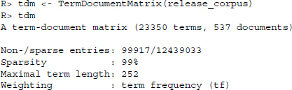
Not surprisingly, the resulting matrix is extremely sparse, meaning that most cells have not a single entry (approximately 99%). In addition, upon closer inspection of the terms in the rows, we find that several are errors that can probably be traced back to unclean data sources. This concern is validated by looking at the figure of Maximal term length that takes on an improbably high value of 252.
10.2.3 Data cleansing
10.2.3.1 Word removals
In order to take care of some of these errors, one typically runs several data preparation operations. Furthermore, the data preparation addresses some of the concerns that are leveled against (semi-)automated text classification which will be discussed in the next section. Several preparation operations have been made available in tm. For example, one might consider removing numbers and period characters from the texts without losing much information. This can either be done on the raw textual data or while setting up the term-document matrix. For convenience of exposition, we will run each of these functions on the original documents.
The main function we will be using in this section is tm_map(), which takes a function and runs it on the entire corpus. To remove numbers in our documents, we call
R> release_corpus <- tm_map(release_corpus, removeNumbers)
We could use the removePunctuation() function to remove period characters. However, this function simply removes punctuation without inserting white spaces. In case of formatting errors of the text this might accidentally join two words. Thus, to be safe, we use the str_replace_all() function from the stringr package. The additional arguments to the function are simply added to the call to tm_map().6
R> release_corpus <- tm_map(release_corpus, str_replace_all, pattern
= ”[[:punct:]]”, replacement = ” ”)
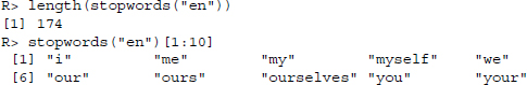
Another common operation is the removal of so-called stop words. Stop words are the most common words in a language that should appear quite frequently in all the texts. However, for the estimation of the topics they should not be very helpful as we would expect them to be evenly distributed across the different texts. Hence, the removal of stop words is rather an operation that is performed to increase computational performance and less in order to improve the estimation procedures. The list of English stop words that is implemented in tm contains more than a hundred terms at the time of writing.
Again, we remove these using the tm_map() function.
R> release_corpus <- tm_map(release_corpus, removeWords, words =
stopwords(”en”))
Next, one typically converts all letters to lower case so that sentence beginnings would not be treated differently by the algorithms.
R> release_corpus <- tm_map(release_corpus, tolower)
10.2.3.2 Stemming
The following operation is potentially of greater importance than those that have been introduced so far. Many statistical analyses of text will perform a stemming of terms prior to the estimation. What this operation does is to reduce the terms in documents to their stem, thus combining words that have the same root. A number of stemming algorithms have been proposed and there are implementations for different languages available in R. Once more, we apply the relevant function from the tm package, stemDocument() via the tm_map() function.7
R> library(SnowballC)
R> release_corpus <- tm_map(release_corpus, stemDocument)
10.2.4 Sparsity and n-grams
Now that we have performed all the document preparation that we would like to include in our analysis, we can regenerate the term-document matrix. Note again that we did not have to perform the single operations on the original texts. We could just as easily have performed the operations concurrently with the generation of the term-document matrices. This is accomplished via the control parameters in the TermDocumentMatrix() function. Note further that there are a number of common weighting operations available that are more elaborate than the mere term frequency. For simplicity of exposition, we will not discuss them in this chapter. Now let us see how the operations have changed the main parameters of our term-document matrix.
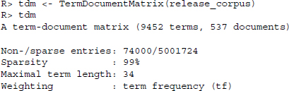
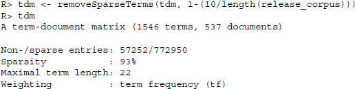
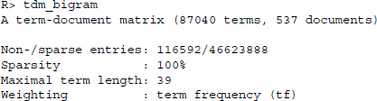
The list of terms has become a lot cleaner and we also observe a more realistic value for the Maximal term length parameter. One more operation that is commonly performed is the removal of sparse terms from a text corpus prior to running the classifiers. The primary reason for this operation is computational feasibility. Apart from that, the operation can also be viewed as a safeguard against formatting errors in the data. If a term appears extremely infrequently, it is possible that it contains an error. The downside of removing sparse terms is, however, that sparse terms might provide valuable insight into the classification which is stripped out. The following operation discards all terms that appear in 10 documents or less.
A common concern that is voiced against the statistical analysis of text in the way that is proposed in the subsequent two sections is its utter disregard of structure and context. Furthermore, terms might have meaning associated to them that resides in several terms that follow one after another rather than in single terms. Moreover, concerns are often voiced that the methods have no way of dealing with negations. While there are diverse solutions to all of these problems, one possibility is to construct term-document matrices on bigrams. Bigrams are all two-word combinations in the text, that is, in the sentence “Mary had a little lamb,” the bigrams are “Mary had,” “had a,” “a little,” and “little lamb.” Within the tm framework, a term-document matrix of bigrams can easily be constructed using the R interface to the Weka program using the RWeka package (Hornik et al. 2009; Witten and Frank 2005).
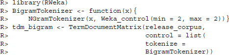
The disadvantages of a term-document matrix based on bigrams is the fact that the matrix becomes substantially larger and even more sparse.
Especially the former point is relevant, as the computational task grows with the size of the matrix. In fact, depending on the specific task, the accuracy of classification using this operationalization does not increase dramatically. What is more, some of the aforementioned concerns are not too severe. Consider the negation problem. As long as negations are randomly distributed they should not greatly influence the classification task.
Before moving on, let us consider an interesting summary statistic of the resulting matrix. Using the findAssocs() function, we are able to capture associations between terms in the matrix. Specifically, the function calculates the correlation between a term and all other terms in the matrix.
In the above call we request the associations for the term “nuclear” where the correlation is 0.7 or higher. The output provides a matrix of all the terms for which this is true, along with the correlation value. We find that the stems “weapon,”“disarma,”“treati,” and “materi” are most correlated with “nuclear” in the press releases that we collected.
10.3 Supervised learning techniques
In this and the following sections, we try to estimate the topical affiliation of the documents in the corpus. A first and important distinction we have to make in this regard is the one between latent and manifest characteristics of a document. Manifest characteristics describe aspects of a text that are clearly observable in the text itself. For example, whether or not a text contains numbers is typically not a quality up for debate. This is not the case for latent characteristics of a text. The topical emphasis of a text might be very well debatable. This distinction is important when thinking about the uncertainty that is part of our measurements. In text classification, we can distinguish between different forms of uncertainty and misclassification.
The first kind of uncertainty resides in the algorithms themselves and can be traced back to limited data availability and a number of simplifying assumptions one typically makes when using the algorithms—not least the assumption that the sequence of the words in the text has no effect on the topic it signals. This point becomes obvious when thinking about the way the data are structured that is underlying our analysis. The so-called bag-of-word approaches hold that the mere presence or absence of a term is a strong indicator of a text's topical emphasis—regardless of its specific location. When creating a term-document matrix of the texts, we discard any sequence information and treat the texts as collections of words. Consider the following example. If you observe that a particular text contains the terms “Roe,”“Wade,”“Planned,”and “Parenthood”you have a decent chance of correctly guessing that the text in some way revolves around the issue of abortion. Moreover, many classifiers rely on the Naïve Bayes assumption. This suggests that observing one term in a text is independent from observing another term. This is to say that the presence of one term contributes independently to the probability that a text is written about a particular topic from all other terms.
Apart from misclassifications based on these simplifying assumptions, there is a second, more fundamental aspect of uncertainty in text classification. This is related to the classification of latent traits in text. As the topical emphasis of a text is not a quantity that is directly observable, there can even be misclassification by human coders. This leads to two challenges in classifying latent traits. One, we are frequently faced with training data that was human-coded and thus might contain errors. Two, it is difficult for us to differentiate between the origins of a misclassification, that is, we cannot be certain whether a text is misclassified for technical or conceptual reasons.
Regardless of the origin, misclassification often poses a formidable problem for social scientists. Oftentimes, we would like to perform text classification and include the estimated categories in a subsequent analysis in order to explain external factors. This second step in a typical research program is frequently hampered by misclassification. In fact, in a real research situation we have no way of knowing the degree of misclassification. If we did have a benchmark, we would not need to perform text classification in the first place. What is worse, it cannot be assumed that classification errors are randomly distributed across the categories, which would pose a less dramatic problem. Instead, the classification errors might be systematically biased toward specific categories (Hopkins and King 2010).
Keeping these shortcomings of the techniques in mind, we now turn to the technical aspects of supervised learners. The supervised in the term reflects the commonality of classifiers in this class that some pre-coded data are used to estimate membership of non-classified documents. The pre-coded data are called the training dataset. It is difficult to provide an estimate of the size of the needed pre-coded data, as the accuracy of classification depends among other things on the length of pre-coded documents and on how well the term usage in the documents is separable, that is, the more the language in the classes differs the easier the classification task. In general, however, the level of misclassification should decrease with the size of the available training data. In addition, it is important to guarantee a sufficient coverage of all categories in the training data. Recall that we discarded press releases from departments that published 20 pieces or less. Even if the overall training data are sizable—which, in our case, it is not—it is possible that one or several categories dominate the training data, thus providing little information on what the algorithm might expect in the less covered categories.
The major advantage of supervised classifiers is that they provide researchers with the opportunity to specify a classification scheme of their choosing. Keeping in mind that we are interested in a latent trait of the document, the topic, we could potentially be interested in a number of other latent categories of documents, say, their ideological or sentiment orientation. Supervised classifiers provide a simple solution to estimating different properties by supplying different training data for the estimation procedure. Before moving on to estimating the topical emphasis in our corpus, let us introduce three supervised classifiers.
10.3.1 Support vector machines
The first model we will estimate below is the so-called support vector machine (SVM). This model was selected as it is currently one of the most well-known and most commonly applied classifiers in supervised learning (D'Orazio et al. 2014). The SVM employs a spatial representation of the data. In our application, the term occurrences which we stored in the term-document matrices represent the spatial locations of our documents in high-dimensional spaces. Recall that we supplied the group memberships, that is, publishing agencies, of the documents in the training data. Using the SVMs, we try to fit vectors between the document features that best separate the documents into the various groups. Specifically, we select the vectors in a way that they maximize the space between the groups. After the estimation we can classify new documents by checking on which sides of the vectors the features of unlabeled documents come to lie and estimate the categorical membership accordingly. For a more detailed introduction to SVMs, see Boswell (2002).
10.3.2 Random Forest
The second model which will be applied is the random forest classifier. This classifier creates multiple decision trees and takes the most frequently predicted membership category of many decision trees as the classification that is most likely to be accurate. To understand the logic, let us consider a single tree first. A decision tree models the group membership of the object we care to classify based on various observed features. In the present case, we estimate the topical category of documents based on the observed terms in the document. A single decision tree consists of several layers that consecutively ask whether a particular feature is present or absent in a document. The decisions at the branches are based on the observed frequencies of presence and absence of features in the training dataset. In a classification of a new document we move down the tree and consider whether the trained features are present or absent to be able to predict the categorical membership of the document. The random forest classifier is an extension of the decision tree in that it generates multiple decision trees and makes predictions based on the most frequent prediction from the various decision trees.
10.3.3 Maximum entropy
The last classification algorithm we have selected is the maximum entropy classifier. We have selected this model as it might be familiar to readers who have some experience with advanced multivariate data analysis. The maximum entropy classifier is analogous to the multinomial logit model which is a generalization of the logit model. The logit model predicts the probability of belonging to one of two categories. The multinomial logit model generalizes this model to a situation where the dependent variable has more than two categories. In our classification task we try to estimate the membership in six different topical categories.
10.3.4 The RTextTools package
Several packages have been made available in R to perform supervised classification. For the present exposition we turn to the RTextTools package. This package provides a wrapper to several packages that have implemented one or several classifiers. At the time of writing, the package provides wrappers to nine different classification algorithms. Using a common framework, the RTextTools package allows a simple access to different classifiers without having to rearrange the data to the needs of the various packages, as well as a common framework for evaluating the model fit.
The most obvious advantage of applying several classifiers to the same dataset lies in the possibility that individual shortcomings of the classifiers cancel each other out. It is often most effective to choose the modal prediction of multiple classifiers as the category that most resembles the true state of the latent category of a text. For simplicity's sake, the present exposition will provide an introduction to three of the classifiers. Nevertheless, all of the algorithms perform an identical task in principle. In each case, the task of the classifiers is to assess the degree to which a text resembles the training dataset and to choose the best fitting label.
10.3.5 Application: Government press releases
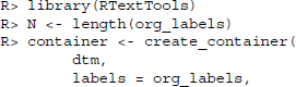
Turning to the practical implementation, we first need to rearrange the data a little so that it conforms to the needs of the RTextTools package. First and foremost, the package takes a document-term matrix as input. So far, we generated a term-document matrix but tm can just as easily output document-term matrices. Appropriately enough the relevant function is called DocumentTermMatrix(). After generating the new matrix we discard terms that appear in ten documents or less. We assemble a vector of the labels that we collected from the press releases using the prescindMeta() function that we have introduced above.
Finally, we create a container with all relevant information for use in the estimation procedures. This is done using the create_container() function from the RTextTools package. Apart from the document-term matrix and the labels we have generated we specify that the first 400 documents are training data while we want the documents 401–537 to be classified. We set the virgin attribute to FALSE, meaning that we have labels for all 537 documents.
The generated container object is an S4 object of class matrix_container. It contains a set of objects that are used for the estimation procedures of the supervised learning methods:
![]()
In a next step, we simply supply the information that we have stored in the container object to the models. This is done using the train_model() function.8
R> svm_model <- train_model(container, ”SVM”)
R> tree_model <- train_model(container, ”TREE”)
R> maxent_model <- train_model(container, ”MAXENT”)
Having set up the models, we want to use the model parameters to estimate the membership of the remaining 137 documents. Recall that we do have information on their membership which is stored in the container. This information is not used for estimating the membership of the remaining documents. Instead, the membership is estimated solely on the basis of the word vectors contained in the supplied matrix.
R> svm_out <- classify_model(container, svm_model)
R> tree_out <- classify_model(container, tree_model)
R> maxent_out <- classify_model(container, maxent_model)
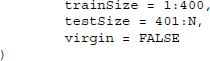
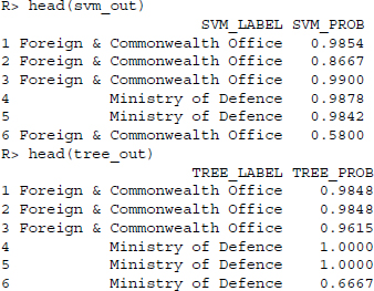
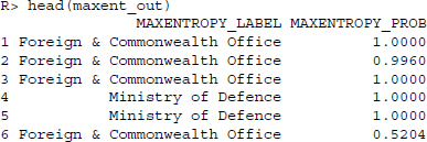
Let us inspect the outcome for a moment. In all three models the output consists of a two-column data frame, where the first column represents the estimated labels and the second column provides an estimate of the probability of classification.
Since we know the correct labels, we can investigate how often the algorithms have misclassified the press releases. We construct a data frame containing the correct and the predicted labels.
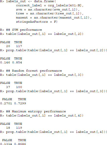
We observe that the maximum entropy classifier correctly classified 119 out of 137 or about 87% of the documents correctly. The SVM fared just a little worse and got 117 out of 137 or about 85% of the documents right. The worst classifier in this application is the random forest classifier, which correctly estimates the publishing organization in merely 100 or 73% of cases.
At the beginning of this section, we have elaborated factors that might be driving errors in topic classification. We suggested that above and beyond technical features of the models, there are conceptual aspects of topic classification that might be driving errors, that is, it might not always be self-evident which category a particular document belongs to. In the present application, there is an additional feature that could potentially increase the likelihood of topic misclassifications. We classified press releases of the British government. For convenience, we selected the publishing organization as a proxy for the document label. However, as governmental departments deal with lots of different issues, it is likely that the announcements cover a wide range of issues. Put differently, we might be able to boost the classification accuracy by including more training data so that we have a more complete image of the departmental tasks.
Having said that, we might in fact want to add that the classification outcome is remarkably accurate, given how little data we input into the classifier. Considering that some categories have a coverage in the training data of little more than 20 documents, it is extraordinary that we are able to get classification accuracy of roughly 80%. This puts the aforementioned question on its head and asks not what is driving the errors in our results but rather what is driving the classification accuracy. One common concern that is voiced against machine learning is the inability of the researcher to know precisely what is driving results. As we are not specifying variables like we are used to from classical regression analysis but are rather just throwing loads of data at the models, it is difficult to know what prompts the results. It is entirely possible that the algorithms are picking up something in the data that is not strictly related to topics at all. Imagine that each departmental press release is signed by a particular government official. If this were the case the algorithms might pick up the different names as the indicator that best separates the documents into the different categories.
In summary, the obvious advantage of supervised classifiers stems from their ability to apply a classification scheme of the researcher's choice. Conversely, the most obvious disadvantage stems from the need to either collect labels or to manually code large chunks of the data of interest that can serve as training data. In the next section, we introduce a way to circumvent this latter disadvantage by automatically estimating the topical categories from the data.
10.4 Unsupervised learning techniques
An alternative to supervised techniques is the use of unsupervised text classification. The main difference between the two lies in the fact that the latter does not require training data in order to perform text categorization. Instead, categories are estimated from the documents along with the membership in the categories. Especially for individual researchers without supporting staff, unsupervised classification might seem like an attractive option for large-scale text classification—while also conforming to the endeavor of this volume to automate data collection.
The downside of unsupervised classification lies in the inability of researchers to specify a categorization scheme. Thus, instead of having to manually input content information, the difficulty in unsupervised classification lies in the interpretation of results in a context-free analysis. Recall that we are estimating latent traits of texts. We established that texts express more than one latent category at a time. Consider as an example a research problem that investigates agenda-setting of media and politics. Say we would like to classify a text corpus of political statements and media reports. If we ran an unsupervised classification algorithm on the entire corpus, it is quite possible that it might pick up differences in tonality rather than in content. To put that in different terms, it might be that the unsupervised algorithms will take the ideologically charged rhetoric of political statements to be different from the more nuanced language that is used in political journalism. One possible solution for the problem would be to run the classifier on both classes of texts sequentially. Unfortunately, running a pure unsupervised algorithm on the two parts of the corpus creates yet another problem, as the categories in one run of the algorithm do not necessarily match up with the categories in a second run. In fact, this poses a more general problem in supervised classification when a researcher wants to match data thus classified to external data that is topically categorized, say, survey responses.
Depending on the specific research goal, it is quite possible that one finds these features of unsupervised classification an advantage of the technique rather than a disadvantage. For instance, the fact that unsupervised methods generate categories out of themselves might be interesting in research that is interested in the main lines of division in a text corpus. Conversely, unsupervised classification often expects the researchers to specify the number of categories that the corpus is to be grouped into. This requires some theoretically driven account of the documents’ main lines of division.
10.4.1 Latent Dirichlet allocation and correlated topic models
The technique that we briefly explore in the remainder of this section is called the Latent Dirichlet Allocation (Blei et al. 2003). The model assumes that each document in a text corpus consists of a mixture of topics. The terms in a document are assigned a probability value of signaling a particular topic. Thus, the likelihood of a text belonging to particular categories is driven by the pattern of words it contains and the probability with which they are associated to particular topics. The number of categories that a corpus is to be split into is arbitrarily set and should be carefully selected to reflect the researcher's interest and prior beliefs.
A shortcoming of the latent Dirichlet model is the inability to include relationships between the various topics. This is to say that a document on topic A is not equally likely to be about topic B, C, or D. Some topics are more closely related than others and being able to include such relationships creates more realistic models of topical document content. To include this intuition into their model, Blei and Lafferty (2006) have proposed the correlated topic model which allows for a correlation of the relative prominence of topics in the documents.
10.4.2 Application: Government press releases
Before turning to the more complex models of topical document content, we begin by investigating the similarity relationships between the documents using hierarchical clustering. In this technique, we cluster similar texts on the basis of their mutual distances. As before, this method also relies on the term occurrences. The hierarchical part in hierarchical clustering means that the most similar texts are joined in small clusters which are then joined with other texts to form larger clusters. Eventually all texts are joined if the distance criterion has been relaxed enough.
For simplicity, we select the first 20 texts of the categories “defence,”“Wales,”and “environment, food & rural affairs”and store them in a shorter corpus.
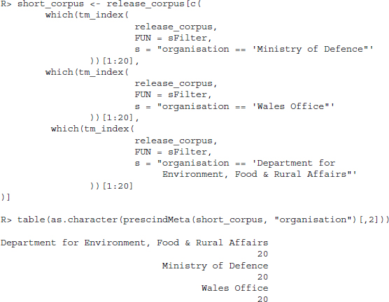
We create a document-term matrix of the shortened corpus and discard sparse terms. We also set the names of the rows to the three categories.
R> short_dtm <- DocumentTermMatrix(short_corpus)
R> short_dtm <- removeSparseTerms(short_dtm, 1-(5/length(short_
corpus)))
R> rownames(short_dtm) <- c(rep(”Defence”, 20), rep(”Wales”, 20),
rep(”Environment”, 20))
The similarity measure in this application is the euclidean distance between the texts. To calculate this metric, we subtract the count for each term in document A from the count in document B, square the result, sum over the entire vector, and take the square root of the result. This is done using the dist() function. The resulting matrix is clustered using the hclust() function which clusters the resulting matrix by iteratively joining the two most similar clusters. The similarities can be visually inspected using a dendrogram where the clusters are increasingly joined from the bottom to the top. This is to say that the higher up the clusters are joined, the more dissimilar they are.
R> dist_dtm <- dist(short_dtm)
R> out <- hclust(dist_dtm, method = ”ward”)
R> plot(out)
The resulting clusters roughly recover the topical emphasis of the various press releases (see Figure 10.1). Particularly toward the lower end of the graph we find that two press releases from the same governmental department are frequently joined. However, as we move up the dendrogram, the patterns become less clear. To a certain extent we find a cluster of the “environment”press releases at one end of the graph and particularly the “Wales” press releases are mostly joined. Conversely, the press releases pertaining to “defence” are dispersed across the various parts of the dendrogram.
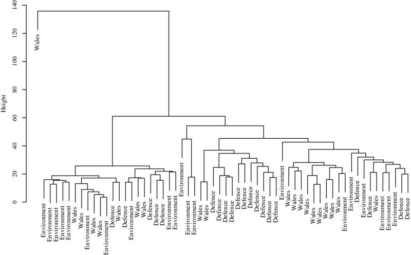
Figure 10.1 Output of hierarchical clustering of UK Government press releases
Let us now move on to a veritable unsupervised classification of the texts—the Latent Dirichlet Allocation. One implementation of the Latent Dirichlet model is provided in the topicmodels package. The relevant function is supplied in the LDA() function. As we know that our corpus consists of six “topics,” we select the number of topics to be estimated as six. As before, the function takes the document-term matrix that we created in the previous section as input.
R> library(topicmodels)
R> lda_out <- LDA(dtm, 6)
After calculating the model, we can determine the posterior probabilities of a document's topics as well as the probabilities of the terms’ topics using the function posterior(). We store the topics’ posterior probabilities in the data frame lda_topics and investigate the mean probabilities assigned to the press releases of the government agencies. We set up a 6-by-6 matrix to store the mean topic probabilities by governmental body.
![]()
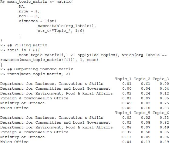
We find that some topics tend to be strongly associated with the press releases from individual government agencies. For example, topic 2 is often highly associated with the Department for Business, Innovation & Skills, topic 5 has a high probability of occurring in announcements from the Foreign & Commonwealth Office. Topic 1 is most associated with the Ministry of Defence. We investigate the estimated probabilities more thoroughly when considering the correlated topic model.
Another way to investigate the estimated topics is to consider the most likely terms for the topics and try to come up with a label that summarizes the terms. This is done using the function terms().
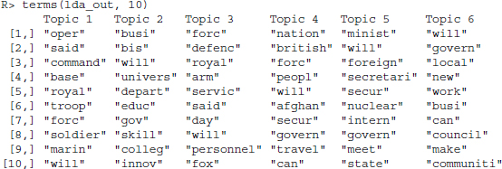
Particularly topics 1, 3, and 4 have a focus on aspects of the military, the terms in topic 5 tend to relate to foreign affairs, the emphasis in topic 6 is local government and topic 2 is related to business and education. This ordering nicely reflects the observations from the previous paragraph. Nevertheless, we also find that the dominance of press releases by the department of defence results in topics that classify various aspects of the defence announcements in multiple topics, thus lumping together the releases from other departments. This is to say that while there is some plausible overlap between the known labels and the estimated categories, this overlap is far from perfect.
Let us move on to estimating a correlated topic model to run a more realistic model of topic mixtures. Again, we select the number of topics to be six since there are six governmental organizations for which we include press releases.
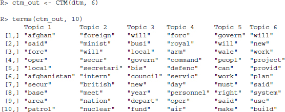
We now find two topics—1 and 4—to be clearly related to matters of defense.9 Topic 2 is associated with foreign affairs, topic 3 with local government. The terms of topic 5 in the correlated topic model strongly suggest Welsh politics. A label for topic 6 is more difficult to make out.
We can plot the document-specific probabilities to belong to one of the three topics. To do so, we calculate the posterior probabilities of the topics and set up 2-by-3 panels to plot the sorted probabilities of the topics in the press releases. The result is displayed in Figure 10.2. Note that to save space we only displayed two of the estimated six topics. We invite you to run the models and plot all posterior probabilities yourself.
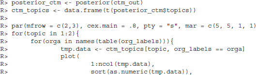
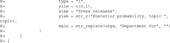
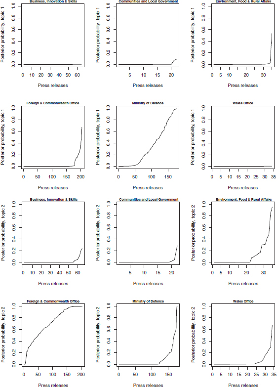
Figure 10.2 Output of Correlated Topic Model of UK Government press releases
The figures are nicely aligned with expectations from looking at the terms most indicative of the various topics. The posterior probability of topic 1 is highest in press releases from the ministry of defense, whereas topic 2 has the highest probability in press releases from the foreign office. In summary, we are able to make out some plausible agreement between our labels and the estimated topical emphasis from the correlated topic model.
Summary
The chapter offered a brief introduction to statistical text processing. To make use of the vast data on the Web, we often have to post-process collected information. Particularly when confronted with textual data we need to assign systematic meaning to otherwise unstructured data. We provided an introduction to a framework for performing statistical text processing in R—the tm package—and two classes of techniques for making textual data applicable as data in research projects: supervised and unsupervised classifiers.
To summarize the techniques, the major advantage of supervised classification is the ability of the researcher to specify the categories for the classification algorithm. The downside of that benefit is that supervised classifiers typically require substantial amounts of training data and thus manual labor. Conversely, the major advantage of unsupervised classification lies in the ability of researchers to skip the coding of data by hand which comes at the price of having to interpret the estimation results ex post.
At the end, we would like to add that there is a vibrant research in the field of automated analysis of text, such that this chapter is potentially one of the first to contain somewhat dated information. For example, some headway has been made to allow researchers to specify the categories they are interested in without having to code a large chunk of the corpus for training data. This is accomplished using seed words. They allow the researcher to specify words that are most indicative of a particular category of interest (Gliozzo et al. 2009; Zagibalov and Carroll 2008).
Further reading
We introduced the most important features of the tm package in the first section of this chapter. However, we have not explored its full potential. If you care to learn more about the package check out the extensive introduction in Feinerer et al. (2008).
Natural language processing and the statistical analysis of text remain actively researched topics. Therefore, there are both numerous contributions to the topic as well as research papers with current developments in the field. For further insight into the topics that were introduced in this chapter take a look at Grimmer and Stewart (2013) for a brief but insightful introduction to some of the topics that were discussed in this chapter. For a more extensive treatment of the topics, see Manning et al. (2008).
A topic that is heavily researched in the area of automated text classification is the classification of the sentiment or opinion in a text. We will return to this topic in Chapter 17 where we try to classify the sentiment in product reviews on http://www.amazon.com. For an excellent introduction to the topic, take a look at Liu (2012).