14
Predicting the 2014 Academy Awards using Twitter
Social media and the social network Twitter, in particular, have attracted the curiosity of scientists from various disciplines. The fact that millions of people regularly interact with the world by tweeting provides invaluable insight into people's feelings, attitudes, and behavior. An increasingly popular approach to make use of this vast amount of public communication is to generate forecasts of various types of events. Twitter data have been used as a prediction tool for elections (Tumasjan et al. 2011), spread of influenza (Broniatowski et al. 2013; Culotta 2010), movie sales (Asur and Huberman 2010), or the stock market (Bollen et al. 2011).
The idea behind these approaches is the “wisdom of the crowds” effect. The aggregated judgment of many people has been shown to frequently be more precise than the judgment of experts or even the smartest person in a group of forecasters (Hogarth 1978). In that sense, if it is possible to infer forecasts from people's tweets, one might expect a fairly accurate forecast of the outcome of an event.
In this case study, we attempt to predict the winners of the 2014 Academy Awards using the tweets in the days prior to the event. Specifically, we try to predict the results of three awards—best picture, best actress, and best actor. A similar effort to ours is proposed by Ghomi et al. (2013). In the next section, we elaborate the data collection by introducing the Twitter APIs and the specific setup we used to gather the tweets. Section 14.2 goes on to elaborate the data preparation and the forecasts.
14.1 Twitter APIs: Overview
Before turning to the Twitter-based forecasts, we provide an overview of the basic features of Twitter's APIs.2 The range of features is vast and we will only make use of a tiny part, so it is useful to get an intuition about the possibilities of Twitter's web services. Twitter offers various APIs for developers. They are documented at https://dev.twitter.com/docs. Using the APIs requires authentication via OAuth (see Section 9.1.11). In the following, we shortly discuss the REST API and the Streaming APIs.
14.1.1 The REST API
The REST API comprises a rich set of resources.3 They offer access to the user's account, timeline, direct messages, friends, and followers. It is also possible to retrieve trending topics for a specific location (WOEID; see Section 9.1.10) or to collect tweets that match certain filter parameters, for example, keywords. Note, however, that there are restrictions regarding possibility to gather statuses retrospectively. There are also rate limits to bear in mind. As both limits are subject to changes, we refer to the documentation at https://dev.twitter.com/docs/rate-limiting/1.1 for details.
The twitteR package provides a wrapper for the REST API (Gentry 2013), thus we do not have to specify GET and POST requests ourselves to connect to Twitter's web service. The package provides functionality to convert incoming JSON data into common R data structures. We list a subset of the package's functions which we find most useful in Table 14.1. For a more detailed description of the package check out Jeff Gentry's helpful introduction at http://geoffjentry.hexdump.org/twitteR.pdf
Table 14.1 Overview of selected functions from the twitteR package
| Function | Description | Example |
| searchTwitter() | Search for tweets that match a certain query; the query should be URL-encoded and special query operators can be used1 | searchTwitter(”#superbowl”) |
| getUser() | Gather information about Twitter users with public profiles (or the API user ) | getUser(”RDataCollection”) |
| getTrends() | Pull trending topics from a given location defined by a WOEID | getTrends(2422673) |
| twListToDF() | Convert list of twitteR class objects into data frame | twListToDF(tweets) |
14.1.2 The streaming APIs
Another set of Twitter APIs are subsumed under the label Streaming APIs. They allow low latency access to Twitter's global data stream, that is practically in real time.4 In contrast to the REST APIs, the Streaming APIs require a persistent HTTP connection. As long as the connection is maintained, the application that taps the API streams data from one of the data flows.
Several of these streams exist. First, Public Streams provide samples of the public data flow. Twitter offers about 1% of the full sample of Tweets to ordinary users of the API. The sample can be filtered by certain predicates, for example, by user IDs, keywords, or locations. For data mining purposes, this kind of stream might be one of the most interesting, as it provides tools to scour Twitter by many criteria. In this case study, we will tap this API to identify tweets that mention the 2014 Academy Awards by filtering a set of keywords. The second type of Streaming API provides access to User Streams. This API returns tweets from the user's timeline. Again, we can filter tweets according to keywords or types of messages, for example, only tweets from the user or tweets from her followings. Finally, the third type of Streaming API is Site Streams which provides real-time updates from users for certain services. This is basically not much different from User Streams but additionally indicates the recipient of a tweet.5 At the time of writing, the Site Streams API is in a restricted beta status, so we refrain from going into more details.
Fortunately, we do not have to become experts with the inner workings of the streaming APIs, as the streamR provides a convenient wrapper to access them with R (Barberá 2013). Table 14.2 provides an overview of the most important functions that we have used to assemble the dataset that we draw on for the predictions in the second part of this chapter.
Table 14.2 Overview of selected functions from the streamR package
| Function | Description | Example |
| filterStream() | Connection to the Public Streams API; allows to filter by keywords (track argument), users (follow), locations (locations), and language | filterStream(file.name = ”superbowl_tweets.json”, track = ”superbowl”, oauth = twitter_sig)’ |
| sampleStream() | Connection to the Public Streams API; returns a small random sample of public tweets | sampleStream(file.name = ”tweets.json”, timeout = 60, oauth = twitter_sig)’ |
| userStream() | Connection to the User Streams API; returns tweets from the user's timeline; allows to filter by message type, keywords, and location | sampleStream(userStream = ”mytweets.json”, with = ”user”, oauth = twitter_sig)’ |
| parseTweets() | Parses the downloaded tweets, that is, returns the data in a data frame | parseTweets(”tweets.json”)’ |
14.1.3 Collecting and preparing the data
To collect the sample of tweets that revolve around the 2014 Academy Awards, we set up a connection to the Streaming API. The connection was opened on February 28, 2014 and closed on March 2, 2014, the day the 86th Academy Awards ceremony took place at the Dolby Theatre in Hollywood.
We began by registering an application with Twitter to retrieve the necessary OAuth credentials which allow tapping the Twitter services. A connection to the Streaming API was established using the streamR interface. The command to initiate the collection was
R> filterStream(”tweets_oscars.json”, track = c(”Oscars”, ”Oscars2014”),
timeout = 10800, oauth = twitCred)
We filtered the sample of tweets using filterStream() with the track option with the keywords “Oscars” and “Oscars2014”, which matched any tweet that contained these terms in the form of hash tags or pure text. We split the process into streams of 3 hours each (60*60*3 = 10, 800 for the timeout argument) to store the incoming tweets in manageable JSON files. All in all we collected around 10 GB of raw data, or approximately 2,000,000 tweets.
After the collection was complete, we parsed the single files using the parseTweets() function in order to turn the JSON files into an R data frame. We merge all files into a single data frame. Storing the table in the Rdata format reduced the memory consumption of the collected tweets to around 300 MB.
R> tweets <- parseTweets(”tweets_oscars.json”, simplify = TRUE)
14.2 Twitter-based forecast of the 2014 Academy Awards
14.2.1 Visualizing the data
Before turning to the analysis of the content of the tweets, let us visually inspect the volume of the data for a moment. Specifically, we want to create a figure of the number of tweets per hour in our search period from the end of February to the beginning of March, 2014.6 The easiest thing to aggregate the frequency of tweets by hour is to convert the character vector in the dataset created_at to a true time variable of type POSIXct. We make use of the lubridate package which facilitates working with dates and times (Grolemund and Wickham 2011). We also set our locale to US English to be able to parse the English names of the months and week days. Chances are that you have to adapt the value in the Sys.setlocale() function to the needs of your machine.7
R> library(lubridate)
R> Sys.setlocale(”LC_TIME”, ”en_US.UTF-8”)
To parse the time stamp in the dataset, we use the function as.POSIXct() where we specify the variable, the timezone, and the format of the time stamp. Let us have a look at the first time stamp to get a sense of the format.
R> dat$created_at[1]
[1] ”Fri Feb 28 10:11:14 +0000 2014”
We have to provide the information that is contained in the time stamp in abstract terms. In this case the stamp contains the weekday (%a), the month (%b), the day (%d), the time (%H:%M:%S), an offset for the timezone (%z), and the year (%Y). We abstract the various pieces of information with the percentage placeholders and let R parse the values.
R> dat$time <- as.POSIXct(dat$created_at, tz = ”UTC”, format = ”%a
%b %d %H:%M:%S %z %Y”)
Now that we have created a veritable time stamp where R is able to make sense of the information that is contained in the stamp, we can use the convenience functions from the lubridate package to round the time to the nearest hour. This is accomplished with the round_date() function where we specify the unit argument to be hour.
R> dat$round_hour <- round_date(dat$time, unit = ”hour”)
We aggregate the values in a table, convert it to a data frame and discard the last entry as we discontinued the collection around the time so it only contains censored information.
R> plot_time <- as.data.frame(table(dat$round_hour))
R> plot_time <- plot_time[-nrow(plot_time),]
Finally, we create a simple graph that displays the hourly tweets in the collection period from February 28 to March 2 (see Figure 14.1). We observe a sharp increase in the volume of tweets in the hours right before the beginning of the Academy Awards.
R> plot(plot_time[,2], type = ”l”, xaxt = ”n”, xlab = ”Hour”, ylab =
”Frequency”)
R> axis(1, at = c(1, 20, 40, 60), labels = plot_time[c(1, 20, 40, 60),
1])
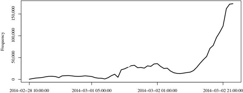
Figure 14.1 Tweets per hour on the 2014 Academy Awards
14.2.2 Mining tweets for predictions
In this part of the chapter, we use the stringr and the plyr packages. We begin by loading them.
R> library(stringr)
R> library(plyr)
Let us inspect one line of the data frame to get a sense of what is available in the dataset:8
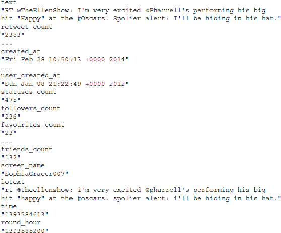
You find that beside the actual text of the tweet there is a lot of the supplementary information, not least the time stamp that we relied upon in the previous section. The last three variables in the dataset are not created by twitter but were created by us. They contain the text of the tweet that was converted to lower case using the tolower() function, as well as the time (time) and the rounded time (round_hour).
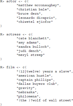
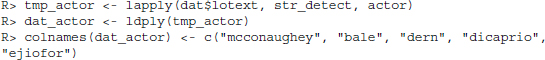
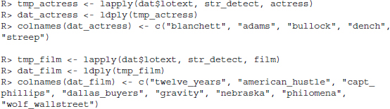
Now, to look for references to the nominees for best actor, best actress, and best picture, we simply create three vectors of search terms. The search terms for the actors and actresses are simply the full name of the actor, in case of the films we created two regular expressions in the cases of “12 Years a Slave” and “The Wolf of Wall Street” as many users on Twitter might have used either variation of the titles. Notice that we have specified all the vectors as lower case as we intend to apply the search terms to the tweets in lower case.9
We go on to detect the search terms in the tweets by applying str_detect() to all tweets in lower case (dat$lotext) via a call to lapply(). The results are converted to a common data frame with ldply() and finally the column names are assigned meaningful names.
To inspect the results, we simply sum up the TRUE values. This is possible as the call to sum() evaluates the TRUE values as 1, FALSE entries as 0.
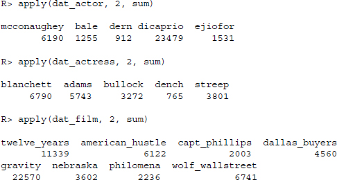
We find that Leonardo DiCaprio was more heavily debated compared to the actual winner of the Oscar for best actor—Matthew McConaughey. In fact, there is a fairly wide gap between DiCaprio and McConaughey. Conversely, the frequencies with which the nominees for best actress were mentioned on Twitter are a little more evenly distributed. What is more, the eventual winner of the trophy—Cate Blanchett—was in fact the one who received most mentions overall. Finally, turning to the best picture we observe that it is not “12 Years a Slave” that was most frequently mentioned but rather “Gravity” which was mentioned roughly twice as often.
In case of the best actor and best actress, we decided to apply a sanity check. As some of the names are fairly difficult to spell, we might potentially bias our counts against those actors where this is the case. Accordingly, we performed an additional search that uses the agrep() function which performs approximate matching.10 The results are summed up and unlisted to get numeric vectors of length five for both categories. Again, we assign meaningful names to the resulting vectors.
![]()
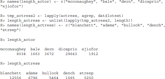
The conclusions remain fairly stable, by and large. Leonardo DiCaprio was more heavily debated than Matthew McConaughey prior to the Academy Awards and the winner of best actress, Cate Blanchett, was most frequently mentioned after applying approximate matching.
14.3 Conclusion
Twitter is a rich playing ground for social scientists who are interested in the public debates on countless subjects. In this chapter, we have provided a short introduction to the various possibilities to collect data from Twitter and making it accessible for research. We have discussed the streamR and twitteR packages to connect to the two main access points for current and retrospective data collection.
In the specific application we have investigated whether the discussion on Twitter on the nominees for best actor and actress as well as best picture for the 2014 Academy Awards in the days prior to the awards reflects the eventual winners. As this book is more concerned with the data collection rather than the data analysis, the technique that was applied is almost banal. We invite you to download the data from the accompanying website to this book and play around with it yourself. Specifically, we invite you to repeat our analysis and apply a sentiment analysis (see Chapter 17) on the tweets to potentially improve the prediction accuracy.