
Please note: The views expressed in this chapter are those of the author and should not be interpreted as those of the Congressional Budget Office.
Before we get started, let me be clear: I get to work with some of the best socioeconomic data in the world. I have access to data provided by the U.S. Social Security Administration (SSA), which provides information on earnings, government benefits (specifically, Social Security benefits), and earnings for a huge number of people over a large number of years. The data is provided to the government through workers’ W-2 tax forms or other government records. By comparison, survey data is often collected from interviews between an interviewer and respondent, but may also be collected online or through computer interfaces in which there is no interaction between the interviewer and interviewee. Administrative data is becoming more widely available in many social science fields, and while that availability is enabling researchers to ask new and interesting questions, that data has also led to new questions about various sources of bias and error in survey data.
Administrative data has both advantages and disadvantages over publicly available survey data. The major advantage is that the administrative data tends to be more accurate than survey data because it is not subject to the typical errors found in survey data. Such errors include:
Nonresponse (the respondent fails to answer a question)
Recall error (the respondent incorrectly answers a question or cannot recall information and fails to answer)
Proxy reporting (one person responds to the survey for another)
Sample selection (the survey sample does not represent the population)
Furthermore, administrative data is typically not imputed (that is, the firm or institution conducting the survey has not inserted values for missing observations) or top- or bottomcoded (that is, variables at the tails of the distribution are not changed to protect the identity of respondents). Finally, administrative data may include a larger number of observations for longer time periods than may be available in survey data.
Administrative data also have several disadvantages, however. First, information is typically available on only a limited set of demographic variables. For example, educational attainment, marital status, and number of children are almost always useful in economic analysis, but are not available in the SSA files I use. In addition, this data does not include earnings that are not reported to SSA (for example, earnings from cash-based employment or acquired “under the table”) or earnings from workers who do not have, or do not report, a valid Social Security number. Unreported earnings may be particularly important for research on, say, immigration policy because many immigrants, especially illegal immigrants, do not have—or have invalid—Social Security numbers.[39]
Let’s put these differences in datasets in some context. A few years ago, two co-authors and I were interested in examining year-to-year changes in individual earnings and changes in household incomes—so-called earnings and income “volatility.”[40] The question of whether people’s (or households’) earnings (or incomes) had grown more or less volatile between the 1980s and 2000s was a hot topic at the time (and, to some degree, still is) and with administrative data at our disposal, we were uniquely suited to weigh in on the issue.[41] To track patterns in earnings and income volatility over time, we calculated the percentage change in earnings/income using three variables:
Earnings/income from the survey data.
Earnings/income from the survey data, excluding observations for which the institution conducting the survey replaced the earnings or income variable with values from a similar person (so-called imputation).
Earnings/income from administrative data matched to survey data (using respondent’s Social Security numbers).
On the basis of previous research, we suspected that the results from the three variables would be roughly the same and that we would find an increase in volatility over time. When we used the raw survey data, we found an increase in volatility roughly between the mid-1990s and the mid-2000s. However, when we dropped observations with imputed earnings or income, we found a slightly slower rate of growth. Then, when we matched the survey data to the administrative records and recalculated the percentage change using the administrative earnings, we found almost no change in volatility over that roughly 20-year period.
This apparently contradictory result made us keenly aware of two shortcomings in the survey data we were using, specifically imputation bias and reporting bias. The strategies you can use to overcome data shortcomings are somewhat limited, but being aware of their existenceand taking as many precautionary steps as possible will make your research better and your results more reliable.
The rest of this chapter describes these two issues—imputations and reporting error—which you might encounter in working with your data. I also discuss four other potential sources of bias—topcoding, seam bias, proxy reporting, and sample selection. The overall message here is to be careful with your data, and to understand how it is collected and how the construction of the survey (or the firm or institution who conducted it) might introduce bias to your data. To address those sources of bias may require time and energy, but the payoff is certainly worth the effort.
High rates of data imputation complicate the use of survey data. Imputation occurs when a survey respondent fails to answer a particular question and the firm or institution conducting the survey may replace values for that record. For example, while a respondent may be perfectly happy to give her name, age, sex, educational attainment, and race, she may be less willing to share how much she earned last year or how many hours she worked last year. There are a number of ways in which the firm or institution can impute missing data; the Census Bureau, for example, uses a variety of methods, the most common being a hot-deck imputation method. (Hot-deck imputation replaces missing values with the value for that same variable taken from a complete record for a similar person in the same dataset.[42]) Imputation rates in the Survey of Income and Program Participation (SIPP; a panel dataset conducted by the Census Bureau) have grown over time, which could further bias research that tracks patterns over multiple years. For example, in work with co-authors, we found that in an early panel of the SIPP, roughly 20% of households had imputed earnings data over a two-year period; in a separate panel about twenty years later, that percentage had risen to roughly 60%.[43]
Although imputing missing data can often result in improved statistics such as means and variances, the use of imputed data can be problematic when looking at changes in certain variables. For example, in our volatility project, we were interested in seeing how people’s earnings and incomes changed over time. Using observations that have been imputed in such an analysis is problematic because observed changes in earnings are not “real” in the sense that they are not calculated from differences in an individual’s reported values between one year and another. (Datasets that follow the same person—or family or household—over time are called longitudinal or panel datasets.) Instead, the calculated change is the difference between actual reported earnings in one period and the imputed earnings in the other. Thus, under a scheme in which earnings are imputed on the basis of some sample average, what you are actually measuring is the deviation from that average, not the change in that individual’s earnings from one period to the next. Alternatively, one could impute the change in the variable of interest, a strategy that might work well for data that has a small variance with few outliers. The exact method by which imputed values are constructed might result in estimates that more strongly reflect the mean or that otherwise introduce bias.
When first exploring a dataset, you should become familiar not only with the data structure and variables available but also with how the survey was conducted, who the respondents were, and the technical approaches that were used to construct the final data file. For example, what happens when people fail to answer a question? Do the interviewers try to ask follow-up questions or do they move quickly to the next question? Was the survey conducted using one-on-one interviews where the interviewer recorded responses, or were respondents asked to fill out a form on their own?
You can deal with imputed data in a number of ways. One can:
Use the imputed data as it is (which is problematic for longitudinal analysis, as previously explained);
Replace the potentially imputed data with administrative earnings records (which, for most researchers, is not a viable option);
Reweight the data to better reflect the population using the sample of survey respondents for whom the variable(s) of interest were not imputed;
Drop the imputed observations (which may bias the results because the resulting sample may no longer be representative).
Economists have approached imputed data in a number of ways. Most studies use imputed data when it is available because it requires less work sifting through the data and maintains the existing sample size. Others, however, drop observations with imputed data, especially those who use longitudinal data.[44]
For longitudinal analysis, the best course of action is probably to drop imputed observations unless an administrative data substitute is available. For cross-sectional analysis, you should tread carefully and test whether the inclusion of imputed observations affects your results. In all cases, you should at least be aware of any imputations used in the survey and how the imputation procedure may have introduced bias to those variables.
Reporting errors occur when the person taking the survey reports incorrect information to the interviewer. Such responses are considered “mistakes” and could be accidental or intentional, but it is impossible to know. Because reporting errors are more difficult to identify, the strategies you can use to address the problem are more limited. In one study, for example, researchers re-interviewed a sample of people and showed that only about 66% of people classified as unemployed in the original interview were similarly classified in the re-interview.[45] Another study compared reports of educational attainment for people over an eight-month period and found that those respondents were most likely to make mistakes in reporting their educational attainment the first time they were surveyed, which suggests that people may become better at taking surveys over time.[46] Of course, in cases in which the survey is conducted only once, there is no chance for the survey respondent to become better at taking the survey and little chance for the researcher to assess the accuracy of responses.
When it comes to measuring earnings, there are two ways in which earnings might differ between survey and administrative data. In the first case, a person works a part-time job for two months, say, at a hardware store early in the year and earns $1,500. When interviewed in December of that year, she tells the interviewer that she had no earnings in the past year; in the administrative data, however, her record shows earnings of $1,500 because that amount was recorded on her W-2. In the second case, a person works full-time shoveling driveways for cash early in the year and earns $500. When interviewed in March, she tells the interviewer that she earned $1,000 shoveling driveways; in the administrative data, however, her record shows no earnings in that year because the shoveling job was paid in cash and no W-2 was filed. In this second case, both datasets are incorrect—earnings were misreported in the survey data and earnings were not reported to the government in the administrative data. These two cases illustrate how errors can occur in either (or both) types of data, and which dataset is better (that is, provides more accurate answers) depends on the question you’re asking. If you’re worried about capturing earnings in the underground economy, an administrative dataset is probably not the best source of information; however, if you’re interested in calculating the Social Security benefits for a group of workers, errors in survey data might cause problems.
These problems are most likely to occur among people at the bottom of the earnings distribution.[47] Figure 10-1 shows the cumulative distribution of earnings in 2009 at $25 increments in the SSA administrative earnings data and the March Current Population Survey (CPS; a monthly survey of over 50,000 households conducted by the U.S. Census Bureau) for people earning less than $5,000 a year. Two observations are immediately evident: First, the cumulative shares of people in the administrative data in each $25 range are about 8 to 15 percentage points above the same point in the CPS, suggesting that the first case described above is probably more prevalent than the second (that is, people underreport their earnings in a survey).[48] The second observation is that respondents in the survey data tend to round reports of their earnings (see the circled spikes in the CPS at thousand-dollar increments), which, depending on the research question may not be a terribly large problem, though in some cases rounding can lead to different estimates.[49]
The challenge a researcher faces with reporting error is that, generally, it is not obvious that it exists. Without comparing one dataset directly with another (for example, merging administrative and survey data together), how can one know whether someone misreported his or her earnings or educational attainment or how many weeks he or she worked last year? Part of dealing with reporting error is digging deep into your data; for example, do you really think a person earned exactly $5,000 last month or worked exactly 2,000 hours last year (50 weeks times 40 hours)? Another part of dealing with reporting error is realizing the strengths and weaknesses of your research question. In some previous work, for example, I was interested in predicting rates of emigration among foreign-born workers (that is, the rate at which people leave the United States). In that case, I inferred emigration rates by following longitudinal earnings patterns over time using administrative data; although that was the strength of the analysis (and, to my knowledge, was the first attempt to use administrative data in that way), the weakness of such an approach is that I clearly missed foreign-born workers who were living and working in the country without authorization (that is, illegal immigrants) and thus may not have filed a W-2.[50]
Although determining whether the dataset you are using is riddled with reporting errors (and whether those errors actually matter) is difficult, being aware of such data shortcomings will take your research further and, importantly, make the validity of your conclusions stronger. Thus, the basic strategy is to be aware and ask key questions:
Is reporting error in your data likely to not be random? If so, your results will be biased.
Do you think reporting error is more likely in some variables than in others?
Can you use other variables to inform sources of potential bias? For example, does everyone with 2,000 hours of annual work also have round earnings amounts? (Perhaps the survey only allows people to check a box of round values instead of asking for exact amounts.)
Does the structure of the survey itself change the probability of reporting error? For example, does the order in which the survey asks questions suggest that people are less likely to answer certain questions because of that order, or might people have some reason for giving less reliable answers at one point in the survey than at some other point?
In sum, reporting errors are difficult to detect, but it’s important to be aware of both the strengths and weaknesses of your data and to try to adjust your model or research questions accordingly.
While imputation bias and reporting error may be two of the largest sources of bias in survey data, there are a number of other issues that can affect the validity and reliability of your data. In this section, I briefly discuss four other sources of bias:
- Topcoding/bottomcoding
To protect respondents’ identities, some surveys will replace extremely high or extremely low values with a single value.
- Seam bias
Longitudinal (or panel) surveys in which changes in survey respondents’ behavior across the “seam” between two interviews are different than the changes within a single interview.
- Proxy reporting
Surveys in which a single member of the interview unit (for example, a family) provides information for all other members.
- Sample selection
Cases in which the very structure or sample of the survey is biased.
There are certain strategies you can use to address or even overcome some of these biases, but in cases in which fixing the source of bias is not possible, once again, it is important to be aware of how the issue might affect your results.

Figure 10-1. Cumulative distribution of earnings for people with positive earnings below $5,000 in the SSA administrative data and CPS, 2009
Tails exist in any distribution, and in the case of earnings or income, for example, those tails can be quite long. To protect the identity of its respondents, the firm or institution conducting a survey might replace extremely high values (topcoding) or extremely low values (bottomcoding) of a variable with a single value. Take, as an example, the Current Population Survey (CPS), a monthly survey of over 50,000 households conducted by the U.S. Census Bureau. In past years, the Census Bureau replaced earnings that exceeded the topcode amount with the topcode amount. For example, prior to 1996, the topcode on earnings was set to $99,999 and so anyone who reported earnings above that cutoff was assigned earnings equal to that value. The effect of that procedure is to create a spike in the distribution of earnings at that level. In more recent years, the Census Bureau has replaced earnings that exceeded some (higher) threshold with average earnings calculated across people with a similar set of characteristics (specifically, gender, race, and work status). This approach has two advantages: one, it does not create a single spike of earnings at the topcode (although it does create several smaller spikes above the topcode); and two, the sum of all earnings is the same with or without the topcode. In the most recent CPS, earnings above the topcode were swapped between survey respondents; this preserves the tail of the distribution, but it distorts relationships between earnings and other characteristics of the earner.
Without access to alternative data sources (either administrative or the raw survey before it is top- or bottomcoded), it is impossible to ascertain the true value of topcoded or bottomcoded earnings. In the case of the CPS, one group of researchers has used administrative data to make a consistent set of topcoded values over time.[51] Other researchers have used administrative data to construct parameters that can be used to assign new values that better reflect the tail of the distribution.[52] If your data has topcodes or bottomcodes and you can infer the expected distribution of the variable, imputing values in this way is a viable approach.
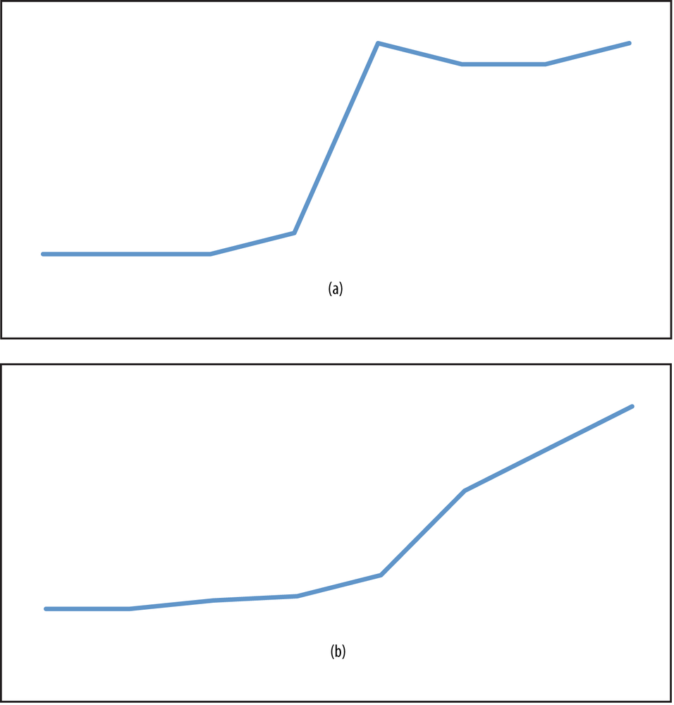
The Survey of Income and Program Participation (SIPP) is a panel dataset (that is, one in which the same people are followed over time) and contains information on approximately 30,000 people for about three to four years. In each panel, respondents are interviewed at four-month intervals about their experiences during the prior four months. One effect of this interviewing scheme is something known as “seam bias,” in which changes measured across the “seam” (that is, from one interview to the next) are much larger than changes measured within a single interview. This can lead variables to jump to a different value every four months (when a new interview occurs) rather than transitioning smoothly as might actually occur. So you might have something closer to Figure 10-2 (a), when instead the pattern should look like Figure 10-2 (b).
To address seam bias, some researchers have suggested making changes to the actual survey, such as encouraging the interviewer to ask respondents to think more carefully about their behavior during the interview interval.[53] Other researchers have suggested strategies that you can use with your data and include choosing specific observations (i.e., specific months), aggregating several observations, or using other more sophisticated statistical techniques.[54]
The SIPP and the CPS both allow proxy reporting; that is, interviews in which a single member of the household (or family) provides information for all other members of the household (or family). For example, the husband of a family of four might provide information on his own earnings and labor force status as well as that of his wife, and the educational attainment of his children. Because the proxy may not know the exact details for everyone in the household, the responses may be incorrect or missing (and thus lead to imputations). If your data includes a variable noting whether proxy reporting exists and who the proxy is, then you can compare nonproxy responses to proxy responses to test whether such reporting biases your estimates.
Another source of bias that can occur is the very type of people surveyed. Some researchers have questioned whether traditional surveys conducted today provide reliable information for a population that is more technologically engaged than in the past. A recent report by the Pew Research Center suggests that in traditional phone-based surveys, contacting potential survey respondents and persuading them to participate has become more difficult. According to Pew, the contact rate (the percentage of households in which an adult was reached to participate in a survey) fell from 90% in 1997 to 62% 2012, and the response rate (the percentage of households sampled that resulted in an interview) fell from 36% to 9% over that same period. Importantly, Pew concludes that telephone surveys (which include landlines and cell phones) that are weighted to match the demographic makeup of the population “continue to provide accurate data on political, social, and economic issues.” However, they also note that “survey participants tend to be significantly more engaged in civic activity than those who do not participate… This has serious implications for a survey’s ability to accurately gauge behaviors related to volunteerism and civic activity.”[55] Again, it is important to ask detailed questions about your data, including how it was constructed and in some cases, and whether the firm or institution conducting the survey has an agenda, in order to increase the validity and reliability of your results.
As mentioned, I get to work with some of the best data you can get your hands on. The comparisons researchers can make between survey and administrative data, which are becoming more widely available (at least in the field of economics), allow researchers to look at people’s behavior in ways that were not available in the past. But those advances have also led to new questions about the accuracy of survey data and the results researchers can reach from models based on that data.
I’ve tried to show you a number of things to be aware of in your data. I typically work with economic data, which contains information on earnings, labor force participation, and other similar behaviors, but the strategies extend to any survey. Methods that firms or institutions use to produce data from surveys—such as imputations, topcoding, and proxy reporting—should always be documented, and as the researcher, you should always be aware of those methods and then decide how they might affect your results. Similarly, respondents may simply make an error in answering the survey, but it is your job to try to determine—or at least to understand—whether those errors impart bias to your results or are simply a hazard of using the best information you have at your disposal.
Bollinger, Christopher R. 1998. “Measurement error in the CPS: A nonparametric look.” Journal of Labor Economics 16, no. 3:576-594.
Bound, John, and Alan B. Krueger. 1991. “The extent of measurement error in longitudinal earnings data: Do two wrongs make a right?” Journal of Labor Economics 9, no. 1:1-24.
Bureau of the Census. 1998. Survey of Income and Program Participation Quality Profile 1998. SIPP Working Paper, Number 230 (3rd edition).
Bureau of the Census. 2001. Survey of Income and Program Participation Users’ Guide (Supplement to the Technical Documentation), 3rd ed. Washington, D.C.
Burkhauser, Richard V., Shuaizhang Feng, Stephen Jenkins and Jeff Larrimore. 2012. “Recent Trends in Top Income Shares in the United States: Reconciling Estimates from March CPS and IRS Tax Return Data.” Review of Economics and Statistics 94, no. 2 (May): 371-388.
Congressional Budget Office. 2007a. “Economic Volatility.” CBO Testimony Before the Joint Economic Committee (February 28).
Congressional Budget Office. 2007b. “Trends in Earnings Variability Over the Past 20 Years.” CBO Letter to the Honorable Charles E. Schumer and the Honorable Jim Webb (April 17).
Cristia, Julian and Jonathan A. Schwabish. 2007. “Measurement Error in the SIPP: Evidence from Administrative Matched Records.” Journal of Economic and Social Measurement 34, no. 1: 1-17.
Dahl, Molly, Thomas DeLeire, and Jonathan A. Schwabish. 2011. “Year-to-Year Variability in Workers Earnings and in Household Incomes: Estimates from Administrative Data.” Journal of Human Resources 46, no. 1 (Winter): 750-774.
Feng, Shuaizhang. 2004. “Detecting errors in the CPS: A matching approach.” Economics Letters 82: 189-194.
Feng, Shuaizhang, Burkhauser, Richard, & Butler, J.S. 2006. “Levels and long-term trends in earnings inequality: Overcoming Current Population Survey Censoring Problems Using the GB2 Distribution.” Journal of Business & Economic Statistics 24, no. 1: 57 - 62.
Gottschalk, Peter, and Robert Moffitt. 1994. “The growth of earnings instability in the U.S. labor market.” Brookings Papers on Economic Activity 2: 217-254.
Haider, Steven J. 2001. “Earnings instability and earnings inequality in the United States, 1967-1991.” Journal of Labor Economics 19, no. 4: 799-836.
Ham, John C., Xianghong Li, and Lara Shore-Sheppard. 2009. “Correcting for Seam Bias when Estimating Discrete Variable Models, with an Application to Analyzing the Employment Dynamics of Disadvantaged Women in the SIPP,” http://web.williams.edu/Economics/seminars/seam_bias_04_06_lara_williams.pdf (April).
Hirsch, Barry T., and Edward J. Schumacher. 2004. “Matched bias in wage gap estimates due to earnings imputation.” Journal of Labor Economics 22, no. 3: 689-772.
Jenkins, Stephen P. 2009. “Distributionally-Sensitive Inequality Indices and the GB2 Income Distribution.” Review of Income and Wealth 55, no. 2: 392-398.
Jenkins, Stephen P., Richard V. Burkhauser, Shuaizhang Feng, and Jeff Larrimore. 2011. “Measuring inequality using censored data: A multiple imputation approach.” Journal of the Royal Statistical Society (A), 174, Part 1: 63-81.
Lillard, Lee, James P. Smith, and Finis Welch. 1986. “What do we really know about wages? The importance of nonreporting and Census imputation.” Journal of Political Economy 94, no. 3: 489-506.
Lubotsky, Darren. 2007. “Chutes or ladders? A Longitudinal analysis of immigrant earnings.” Journal of Political Economy 115, no. 5 (October): 820-867.
McGovern, Pamela D. and John M. Bushery. 1999. “Data Mining the CPS Reinterview: Digging into Response Error.” 1999 Federal Committee on Statistical Methodology (FCSM) Research Conference. http://www.fcsm.gov/99papers/mcgovern.pdf.
Moffitt, Robert A., and Peter Gottschalk. 1995. “Trends in the Covariance Structure of Earnings in the U.S.: 1969-1987.” Johns Hopkins University. Unpublished.
Pew Research Center. 2012. “Assessing the Representativeness of Public Opinion Surveys.” http://bit.ly/SIhhKP (May).
Pischke, Jorn-Steffan. 1995. “Individual Income, Incomplete Information, and Aggregate Consumption.” Econometrica, 63: 805-840.
Roemer, Marc I. 2000. Assessing the Quality of the March Current Population Survey and the Survey of Income and Program Participation Income Estimates, 1990-1996. Income Surveys Branch, Housing and Household Economic Statistics Division, U.S. Census Bureau (June 16).
Schwabish, Jonathan A. 2007. “Take a penny, leave a penny: The propensity to round earnings in survey data.” Journal of Economic and Social Measurement 32, no. 2-3: 93-111.
Schwabish, Jonathan A. 2011. “Identifying rates of emigration in the U.S. using administrative earnings records.” International Journal of Population Research vol. 2011, Article ID 546201, 17 pages.
Shin, Donggyun, and Gary Solon. 2009. “Trends in Men’s Earnings Volatility: What Does the Panel Study of Income Dynamics Show?” Michigan State University. Unpublished.
Ziliak, James P; Hardy, Bradley; Bollinger, Christopher. 2011. “Earnings Volatility in America: Evidence from Matched CPS,” University of Kentucky Center for Poverty Research Discussion Paper Series, DP2011-03 http://www.ukcpr.org/Publications/DP2011-03.pdf (September).
[39] See, for example, Lubotsky (2007) and Schwabish (2011).
[40] Perhaps the most technical presentation of our work was published in Dahl, DeLeire, and Schwabish (2011). Interested readers should also see Congressional Budget Office (2007a, 2007b).
[41] I would be remiss if I didn’t add citations to at least a few seminal works in this area: Gottschalk and Moffitt (1994), Moffitt and Gottschalk (1995), Haider (2001), and Shin and Solon (2009).
[42] Bureau of the Census (2001).
[43] Dahl, DeLeire, and Schwabish (2011). In that study, we found that 21% of households had imputed earnings in 1985, 28% in 1991, 31% in 1992, 33% in 1993, 35% in 1994, 54% in 1998, 60% in 2002, and 46% in 2005.
[44] See, for example, Bound and Krueger (1991); Bollinger (1998); and Ziliak, Hardy, and Bollinger (2011); Lillard, Smith, and Welch (1986); Hirsch and Schumacher (2004); and the discussion in Dahl, DeLeire, and Schwabish (2011).
[45] McGovern and Bushery (1999).
[46] Feng (2004).
[47] They are also problematic at the top of the distribution, but the percentage differences are most likely smaller.
[48] That finding is supported in, for example, Cristia and Schwabish (2007).
[49] See Roemer (2000), Schwabish (2007), and Cristia and Schwabish (2007).
[50] Schwabish (2011).
[51] See, for example, Jenkins et al. (2011) and Burkhauser et al. (2012).
[52] Feng, Burkhauser, and Butler (2006) and Jenkins (2009).
[53] Bureau of the Census (1998).
[54] See, for example, Pischke (1995) and Ham, Li, and Shore-Sheppard (2009).
[55] Pew Research Center (2012). Sample selection might also occur in the form of different technologies used to ask questions of survey respondents. For example, surveys that ask respondents to use a computer to respond might result in less-reliable responses from elderly respondents, or surveys that only ask questions in a single language might not be representative of certain communities.