
![]()
Querying Data in Neo4j with Cypher
When you’ve spent the time building up a data structure, planning the best relationships for the different node types, and of course collecting the data, you want results. Cypher allows us to take all of the hard work in building up a good dataset, and use that to give a better experience for users, or supply accurate recommendations. There are a lot of ways to analyze your data to show trends and gain insight into those that supplied it. Whether that is from a user making orders to generate more accurate recommendations on an e-commerce website or to a blog user seeing their most popular posts by seeing which of them has the most comments. There are many uses for data, and we’re going to cover how to use Cypher to get the data you need for a multitude of situations.
To best showcase the wide range of Cypher’s capabilities, there will be two main examples used. The first, will be a Pokémon-based example, composed of user-submitted data. The second, will be a location-based example, composed of generated data based on various locations. These two approaches demonstrate how Cypher can do both recommendation-based queries and distance-based ones as well. Both of these examples demonstrate the power of Cypher, and these can be adapted to various situations, including e-commerce, which will also be covered. The e-commerce application is an obvious choice for demonstrating recommendations, so aspects of the logic applied in the Pokémon example will also be applied to e-commerce.
With that out of the way, it’s best to just dive right in to the Pokémon example, to demonstrate how Cypher be used to generate recommendations, and of course, the e-commerce application.
Recommendations, Thanks to Pokémon Data
I wanted to find an interesting way to generate data for use in the book and decided to get the community involved in supplying data. To as many people involved as possible, I decided to try and widen my audience, and make it something that would apply to anybody; anybody that liked Pokémon, that is. I’m a big fan of Pokémon, and figured I’d try to involve that, plus I know I’m not the only person who likes it. The idea of the application came from the original Pokémon slogan, Gotta catch em’ all! Why not make that the objective? With the idea in place, I had to then build a website to make it happen.
Getting the Data, the Website Used
After seeing the slogan, it seemed a good idea to make a game out of catching them all, so that’s just what happened. The idea was, you’d get one shot to randomly catch them all, but you could pick four Pokémon to reserve, so you could make sure you had your favorite. There were a couple of rules when it came to choosing these reserved Pokémon, but I’ll get to those in a moment. While they were playing the game, it made sense to try to get some information about the user, which could be used when analyzing the data. The data recorded was picked for a reason, and all kept optional (most of the time, but we’ll get to that) so it was all fair. This essentially meant that each user or Trainer (as they were labeled in Neo4j) that submitted data would get a random sample of Pokémon, ranging between 1 and 200. In addition to that sample, they would also have four Pokémon they’d reserved, and if they’d submitted it, some other personal information to go with this sample. As far as the user was concerned though, they’d just pick four Pokémon, fill in a form, then be presented with a page of Pokémon they’d caught.
The Pokémon that could actually be caught were the first 151, so there’s a chance to catch Mew, as Mew is the 151st Pokémon, and was added after the initial release, for those that are interested, that is. That means that there is an actual chance to get all 151, as you get can get over 151 chances, and you already pick 4 to begin with.
Data Being Gathered
Of course I wanted to make sure the website was fun, but I still wanted to gather data that could be analyzed and was of course above all else, useful. Although supplying the data is entirely optional, each user had the option to submit the following information, supplied in Table 7-1.
Table 7-1. The personal data recorded for those who submitted on pokemon.chrisdkemper.co.uk for use in the book and the reasoning for each
Data item | Reasoning |
|---|---|
Nickname | This was the best means of identifying a user if they wanted to be mentioned in the book. |
The e-mail address here was only used to contact those who were mentioned, just to let them know their nickname would be used (or not, as it seems). | |
Gender | There were only four Pokémon selected by the user, but gender is still a good value to have when it comes to analyzing data. |
Age | Having an age for the user allows some nice range-based queries depending on the range of the data available, so again, it is useful to have. |
Each item of data recorded had its own benefit, and of course is only used for this chapter. The e-mail data stored has since been removed, as the only reason it was needed was to contact those who’ve been featured in the book, and in a couple of cases, when they weren’t, spam is always a problem, even if you use a reCAPTCHA.
Keeping the Spam Under Control
To try to keep spam users down to a minimum, I implemented a reCAPTCHA on the website, which is Google’s offering in the fight against spam. If you’ve never come across one, it’s just a checkbox you need to check if you’re human, and it may also ask you to identify some similar images. Although technically spam data would just be anonymous data, I wanted to avoid 100% of the data being spam. If I’d wanted automated data, I’d have just scripted that.
The other advantage of the reCAPTCHA application means that although there will be anonymous data, it’s still user-submitted anonymous data. This means, that the Pokémon characters that have been reserved, have all been picked by an actual person, provided the reCAPTCHA has been keeping the spam bots at bay.
Keeping the spam bots at bay was a priority, but I also didn’t want to use completely anonymous data, because as I said earlier, I could have generated that. To get around this, I put in a validation check to ensure there wasn’t more than 50% anonymous submissions already in the database.
If a user posted without a nickname, and 50% of the existing entries were anonymous, then they had to add a nickname to submit their data. They could still have anything as a username, nothing was unique, just as long as it was populated. The idea was that having another look at the form may allow for some additional data to be added, rather than the now required, nickname.
I used Cypher to pull out two figures to help with the calculation, the total submissions, and the number of anonymous submissions. The query used to achieve this is as follows.
MATCH (t:Trainer)
MATCH (a:Trainer {nickname: ’anonymous’})
RETURN count(DISTINCT t) AS total, count(DISTINCT a) AS anon;
The main thing to note in the above query is the use of DISTINCT, which ensures each node is only counted once, otherwise you run into a duplication problem. This duplication problem comes from count using both match statements to do the count, even though it shouldn’t. Thanks to the multiple matches, this results in the same result for both values. To show this, first will be Figure 7-1, which will be the results without DISTINCT, and then Figure 7-2 soon after, show the results with DISTINCT.
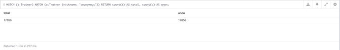
Figure 7-1. Showing the results of the Cypher query being used without DISTINCT
You can see in Figure 7-2 that the results are the same for both values, which is of course useless to us. To make this data actually useful, DISTINCT is added as shown in Figure 7-2.

Figure 7-2. Showing the results of the Cypher query with the use of DISTINCT
You can see here there are now unique values being returned for each, which is much more useful. The interesting thing here are the values being returned. The first value was 6076 for both `total` and `anon`, and the actual values were 98 and 82, for `total` and `anon` respectively. The two unique values multiplied together: 98 * 62 equals the first value, 6076. This gives some reasoning behind the initial value, but also shows the importance of DISTINCT, in the times it’s needed.
With the Cypher side out of the way, after the values are returned, they’re used to work out a percentage, and if it’s over 50%, the user cannot submit anonymously. If this user submitted data anonymously, with an unrounded percentage of 63.2, they’d have to add a nickname to get their shot at catching them all.
To best understand how the queries work, you must first know the data you are querying against. In this case, all 151 Pokémon were imported into the database, with various different properties. An example of Bulbasaur, the first Pokémon (in terms of Id number, 1, that is) can be seen in Table 7-2.
Table 7-2. Bulbasaur’s properties within the database
Property | Value |
|---|---|
Name | Bulbasaur |
Index | 1 |
Height | 7 |
Weight | 69 |
Type | [poison, grass] |
The data for each Pokémon was obtained from the Pokeapi, available at http://pokeapi.co. I wrote a script to import the Pokémon into Neo4j, based on the Id numbers, and then picked these properties to use. The API has a lot available to use, so it’s worth looking at if you’re doing a Pokémon-related project. The type(s) I wanted to store as an array, so they could be used as a filter later. The Pokeapi was a bit too verbose with the information it had regarding the types, at least for my needs, so I had to trim it down to just the names of the types.
With the Pokémon nodes, it was then just a case of relating a Trainer to the Pokémon as needed. There are two relationship types used, RESERVED and CAUGHT. The former, are the Pokémon that are picked by the user, and the latter, are the Pokémon that have been randomly assigned. This helps do some interesting queries later, including the most reserved Pokémon.
When a user submits their data, a Trainer node is created, with any information they supply attached as properties to the node. The Trainer is then related to their RESERVED Pokémon, with a RESERVED relationship, and the website assigns the CAUGHT relationships as needed. This database is one that is relationship heavy, as one user can have up to a maximum of 204 relationships, provided they get the highest achievable random value. An example of how a Trainer’s relationships will be displayed can be seen in Figure 7-3, where a random node has been selected, and its structure can be seen.
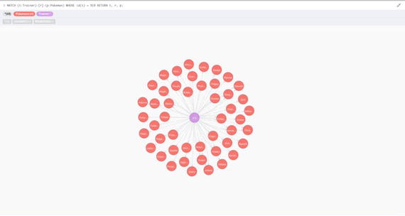
Figure 7-3. The structure of Trainer node in the database, in this case node 919
As you can see, Figure 7-3 shows that one Trainer has many relationships to Pokémon, in this case 54, to 48 different Pokémon. The query used to achieve this was as follows:
MATCH (t:Trainer)-[r]-(p:Pokemon)
WHERE id(t) = 919
RETURN t, r, p;
The query is just a normal relationship-based query, with a WHERE clause to filter it down to the trainer with the node id of 919. This example node shows how the relationships will work within the application, so when we get to the Cypher queries, the use of Pokémon and Trainer Labels will make a little more sense.
Rules for Choosing Pokémon
To make things a little bit more interesting there was a catch when it came to selecting which Pokémon you were allowed to pick. The first rule was that you were only allowed one starter Pokémon, or any evolution of that Pokémon. If you’ve ever played the games, you’ll know that you only get a choice of one of three starter Pokémon, so this rule was to bring some of those feelings back. To give some extra choice, I allowed the inclusion of evolutions of the Pokémon, so you could pick Charmander, or Charizard for your starter, if you even wanted to pick one.
This rule means that it’s possible to see the most popular starter Pokémon, including their evolutions, which is interesting for analysis. There was a similar rule applied for Fossil-based Pokémon, and also Legendary Pokémon for their uniqueness. The rules don’t have any real impact on the process, it just allows for additional analytics points. When the actual Pokémon are picked by the system, these rules don’t apply, so it’s a 1/151 chance to get any particular Pokémon.
Querying the Data
With all the data collected (at the last point it could be before printing) it’s now possible to use that data and work out a lot of different things. Although this dataset is mostly random, a lot can be learned from it, as the concepts used here can be applied to other things where the data won’t be so random, such as e-commerce. A number of different values will be worked out, with the Cypher used to retrieve them, and of course, the results of the queries on the data. In addition to taking data for analytics, it’s also possible to make recommendations for individual `Trainers` (as they’re labeled in Neo4j in the database) for different Pokémon they could catch, based on which type they have the least of, for example.
To make things easier, the queries will be divided into two groups. The first group will be queries based on the dataset as a whole, so the more analytical aspect. The second group will be recommendation based, and will be applied to individual trainers. Let’s get right into it, starting with the analytics side of things.
Analyzing the Data as a Whole
Whether your dataset is big or small, being able to analyze it helps provide insight into what you’re actually collecting, and you can then use the results to help streamline your application. In this case we have a lot of random sets of Pokémon, based on anonymous, and non-anonymous data. Once again, the queries can be broken down into two groups, anonymous (so not using, nickname, gender, or age) and non-anonymous (using the values collected to filter data) respectively. Within each group there will be a number of queries based upon the group they’re in, and the results of those queries. Let’s just dive into the anonymous data sample, and do some queries on all of the data.
These queries are ones that applied to the dataset as a whole, without taking any of the properties of the Trainer nodes (data submitted, along with their reserved Pokémon) into account. The first query will be totaling which Pokémon was the most popular overall, so let’s get to it.
Most Popular Pokémon
In terms of trainers there are two kinds of Pokémon in the database, those they caught by means of them being randomly generated, and those they reserved. For this query, we don’t care, we just want to know which is the most popular Pokémon between the Trainers, which in Cypher terms, is like this:
MATCH (:Trainer)--(p:Pokemon)
RETURN p.name AS name, count(p.name) AS count
ORDER BY count DESC
LIMIT 10
This query then gives the results seen in Figure 7-4.
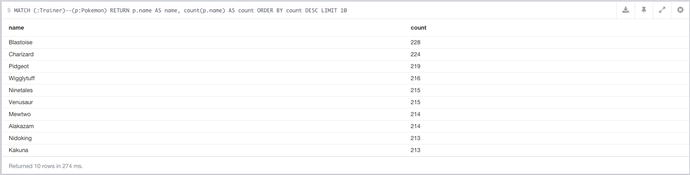
Figure 7-4. The first 10 results of the most popular Pokémon query
We’ll get to the results in a minute, but the query itself isn’t too complicated. First, we need the Pokémon that a Trainer has caught. We could have achieved this by using ()-[]-(p:Pokemon) which gets any Trainer to Pokémon, regardless of direction or type. This does work, but being specific in Cypher queries is always good for performance, and specifying the Trainer label helps speed up the query, even if only marginally. Since the relationship isn’t considered here, that can also be dropped from the query, resulting in (:Trainer)--(p:Pokemon) being used.
After returning the data, it’s time to arrange it in descending order, which is achieved with ORDER BY count DESC. Rather than getting all of the data, it’s better to get a small subset, which in this case, was 15.
It’s not surprising to see all of the top-level Pokémon in the list. Although these results are random at this stage, it’s still good to see. That’s enough about those, let’s move on to more specific queries.
Who Caught the Most
Since the website was based around catching them all, finding out if anybody did is a big deal, so let’s get started on the query. What we essentially need to see here is which trainers got the most relationships, but only unique relationships, to remove the duplicates. This is achieved with the following Cypher query:
MATCH (t:Trainer)--(p:Pokemon)
RETURN id(t) AS id, t.nickname AS name, count(DISTINCT p.name) AS count
ORDER BY count desc
LIMIT 10
Using this query, the following results were obtained, which can be seen in Figure 7-5.
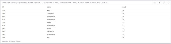
Figure 7-5. The results of the query showing which users caught the most Pokémon
This query is a little difficult, and the most important part is the use of the id function. The match here gets the Trainers that have caught Pokémon, regardless of their type, as we want them all. Next the data is just returned, with DISTINCT p.name being counted. Without the id function in the query, this count would actually make all of the values of ’t.name` unique, and then sum the corresponding values. This means that rather than multiple anonymous values, there would be one super anonymous value, with all of the various count totals added to it. The id function then ensures each node is evaluated individually, in this case keeping the duplicates.
The Results
It was user `KeV` that managed to get the top spot here. Sadly there wasn’t a score of 151, but I’m sure, given enough shots, somebody would get it eventually. If you invert this query, it reveals that the lowest score was a tie between CJ, schlocke, and hill79 all had a tie at 5. That’s unlucky, I blame Team Rocket.
Most Popular CAUGHT and RESERVED Pokémon
We’ve already seen the results for the most popular Pokémon, but we’ve yet to see the values for the specific types. In this case, we’ll be covering the most popular randomly caught Pokémon. This really provides insight into how the balance was between the different numbers, so essentially if it was actually fair. The query isn’t too different from the previous one, it just has a small change. The full query is as follows:
MATCH (:Trainer)-[r:CAUGHT]-(p:Pokemon)
WITH count(p.name) AS total_count
MATCH (:Trainer)-[r:CAUGHT]-(p:Pokemon)
WITH p.index AS id, p.name AS name, count(p.name) AS total, total_count
RETURN id, name, total, total_count AS `Total Caught`
ORDER BY total DESC
LIMIT 10
With this query, you then get the results seen in Figure 7-6.
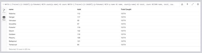
Figure 7-6. Shows all of the CAUGHT Pokémon, with an included total
The query used to generate these results is a little different from the previous ones, as it has multiple MATCH statements. The first MATCH statement is to get the total number of CAUGHT Pokémon within the database, which could be used to work out the percentage of the total each Pokémon has. This value could have been obtained from its own query of course, but this way it’s included on every result row, so if it’s needed it’s there.
To ensure both queries work as expected, WITH is utilized, to help only pass the relevant information to the rest of the query. You can see that the count of `p.name` has been aliased to `count` using AS. In the next statement, another WITH is used, which essentially just passes these values to the RETURN clause, so they can be returned. When using WITH, you’ll see that the `count` from the first statement is also included in the WITH of the second. Without this inclusion, `count` would not be defined for use in the return statement.
Another thing to mention about the first query is the value it returns. If you ran that query by itself, it would be like so:
MATCH (:Trainer)-[r:CAUGHT]-(p:Pokemon)
RETURN count(p.name) AS `Total Caught`
Since only a count is returned, and nothing node related, then all of the values that would be returned if the count was specific to the node (just like in the second part of the previous query) are added together, and returned as one total value. The rest of the query just gets some additional information about the Pokémon being returned, and also orders the results by the most counted, in descending order.
Given how the relationships are set up within the database, determining the most popular RESERVED Pokémon, rather than the most random CAUGHT Pokémon requires one change, the relationship type. The modified query can be seen below.
MATCH (:Trainer)-[r:RESERVED]-(p:Pokemon)
WITH count(p.name) AS total_count
MATCH (:Trainer)-[r:RESERVED]-(p:Pokemon)
WITH p.name AS name, count(p.name) AS total, total_count
RETURN name, total, total_count AS `Total Reserved`
ORDER BY total DESC
LIMIT 10
Depending on the use case, it may be possible to remove total count from the query as we’re looking at this data as user-selected data, so whomever is on top is the most popular. That being said, having the total allows us to work out the percentage of the total each value was, so whether or not this query can be trimmed down can be decided. The modified query gives the results seen in Figure 7-7.
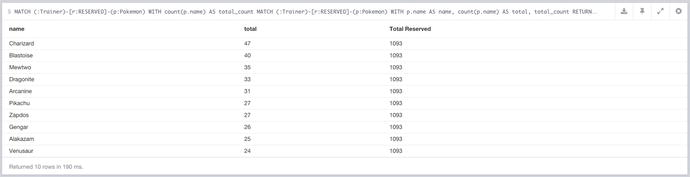
Figure 7-7. The results of the most popular RESERVED Pokémon query
Most Popular Pokémon Type
Each Pokémon has at least one type within the database; in some cases, two. These values have been stored in Neo4j as an array of string values, which means they can be used within queries, provided the values are treated the same as they are stored, so in this case, strings. The query now needs to take the types from all of the caught Pokémon, and ensure the list is ordered by the most popular type. That’s enough talk, let’s get straight into it. The Cypher for the query can be seen below.
MATCH (:Trainer)--(p:Pokemon)
WITH p.type AS types
UNWIND types AS type
RETURN type, count(type) AS total
ORDER BY total DESC
LIMIT 10
As we’re only interested in Pokémon data, the Trainer alias can be left off as it’s not used. The interesting part of the query comes with the use of UNWIND, which allows each individual type to be counted, rather than treating multiple values as one row. If the above has been run without the UNWIND, then any time a Pokémon had more than one type, this combination would be counted as one type, rather than two different types.
We already know Bulbasaur’s types from previously in the chapter, which are poison and grass. Without the use of UNWIND, the combination of poison and grass would be counted as one value. Essentially, the use of UNWIND allows each item in the array to be evaluated as an individual item.
Thanks to the combination of WITH and UNWIND, it means that when the data has to be counted, it’s already just a huge list of types, so they just need to be counted, ordered, and of course the type itself needs to be returned, so the numbers make sense. This query gives the result shown in Figure 7-8.
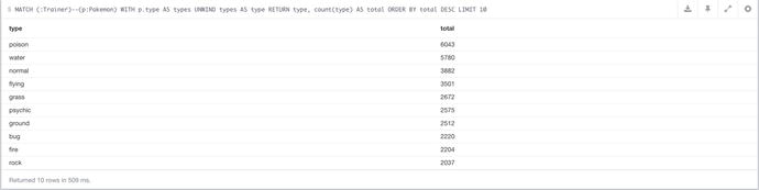
Figure 7-8. The results of the query to determine the most popular types within the database
This query could be modified slightly to give more specific result sets depending on the use case, so if you wanted to know the most popular type within RESERVED Pokémon, just add a relationship constraint to the query. It could be also possible to see what is the most popular type among the Pokémon, regardless of the Trainer input, which would look like so:
MATCH (p:Pokemon) WITH p.type AS types UNWIND types AS type
RETURN type, count(type) AS total
ORDER BY total DESC
LIMIT 10
This allows you to see which are the most and least popular Pokémon types, so if you wanted to catch specific types to strengthen your team, that could be done using this query. The only real change in this query is the removal of the Trainer relationship, as we can just query the Pokémon nodes directly to get the types in this case. Speaking of the results of the Trainer version of the query, let’s go through those.
All of the previous queries have been based on completely anonymous results, but the database isn’t all anonymous, so it’s time to look at what data we have available. As mentioned earlier, the fields recorded were `nickname`, `gender`, `email`, and `age`. Really, out of these fields, there are only two that can be of any real use, which are `gender` and `age`. With these fields, it allows the data to be categorized by age ranges, and of course, gender.
Of course, had I collected more data, such as location, there would have been more granular results, but with age and gender values, this still gives some values. We’ll be performing a number of queries using these values to help filter down the results, and give some insight into those that submitted their data to be used.
Popular Pokémon Filtered by Gender
We’ve already done a query to work out the most popular Pokémon, so with a couple of alterations, it can be modified to return gender-specific values. The resulting Cypher query can be seen below.
MATCH (t:Trainer)--(p:Pokemon)
WHERE t.gender = ’male’
RETURN p.name AS name, count(p.name) AS count
ORDER BY count DESC
LIMIT 10
In this query, we need to use the values of the Trainer node, so `t` has to be in to supply data for the filter. In terms of the stored data, the gender property will be either set to `male`, or `female`, or be null, as it only gets set if there’s a value to set. In the WHERE, it’ll remove null values by default, unless specified otherwise. Since we don’t want the null values, then the basic WHERE does the job. To get the female results it’s just a case of swapping out `male` for `female` in the query. You can see the results of this query in Figure 7-9.
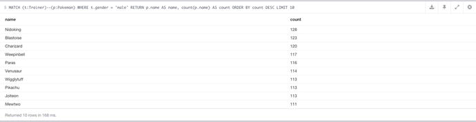
Figure 7-9. The results of most popular Pokémon query, filtered by gender, in this case `male`
Switching the results to filter by `female` rather than `male` gives the results, seen in Figure 7-10.
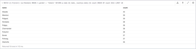
Figure 7-10. The results of most popular Pokémon query, filtered by gender, in this case `female`
Popular Pokémon Filtered by Age
Having access to age is a brilliant way to filter data, as it allows you to filter by age ranges, as well as an individual age. If you want to filter by an age range, you can either have these preset, or decide them based on what values are available within your data. In this case, we’ll be checking the ages submitted, and using those values to build up acceptable ranges on which to base the main query. First, we need all the ages that have been submitted and the counts for these, which in Cypher terms looks like this:
MATCH (t:Trainer)
RETURN t.age AS age, count(t.age) AS count
ORDER BY count DESC
In addition to giving the different range of ages within the data, it also gives the most popular, which although it’s not particularly useful in this case, being able to identify your key age or age group is always a good thing. To get this value, the query just needs to be ordered by the `count`, rather than the `age`. The results of the query can be seen in Figure 7-11.
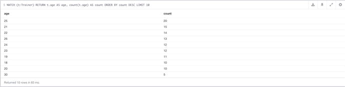
Figure 7-11. A query to show all of the submitted ages within the database
With a slight modification it could also be possible to use an age range with the query, which would look like so:
MATCH (t:Trainer)--(p:Pokemon)
WHERE t.age > 18 AND t.age < 21
RETURN p.name AS name, count(p.name) AS count, t.nickname
ORDER BY count DESC
After covering queries that were based on the data as a whole, it’s time to get to a more personal level and recommend different things to the Trainers. Each Trainer node has at least 4 relationships to different Pokémon within the system, which means there are still 147 different choices available. Unless you’re like Ash (the main character in Pokémon) and want to ‘Catch them all’, you may want to apply some strategy to the Pokémon you catch. This is where the recommendations come in.
Recommend Pokémon, Based on Type
As a trainer, it would be nice to know what types you have the most of, because this shows you which areas you may need to build on. Even if that’s of no use to you, knowing which areas you are weakest in could be, so let’s get to working that out, shall we? A node id used previously was 919, so we’ll use it again here. Trainer 919 needs the types of all of the Pokémon they have caught, and the counts for them.
MATCH (t:Trainer)-[]-(p:Pokemon)
WHERE id(t) = 919
UNWIND p.type AS type
RETURN type, count(type) AS total
ORDER BY total ASC
With the query in place, Trainer 919 gets the results seen in Figure 7-12. In this query, we’re selecting Trainer 919 using WHERE id(t) = 919 after getting all of the Pokémon related to said Trainer. Since the type is an array, it needs to be iterated, which is where UNWIND comes in. After that `type`, and the count of `type` are returned. Thanks to count aggregating the `type` values to count them, it also removes the duplicates from the rows, which is useful in this case.
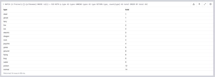
Figure 7-12. The types and their counts for the Pokémon Trainer 919 has
The only bad thing about this list is there are no zero values, so what if Trainer 919 doesn’t have a type at all? Well, there’s an easy way to check, we just need to get all of the different types that the Pokémon have, look at the total. Using Cypher, that looks like this:
MATCH (p:Pokemon)
UNWIND p.type AS type
RETURN DISTINCT type
This query gives the results seen in Figure 7-13. This query is a slimmed down version of the one used above. In this case, because the count is being used in the return, duplicate values will be returned, so to get around that, DISTINCT is used.
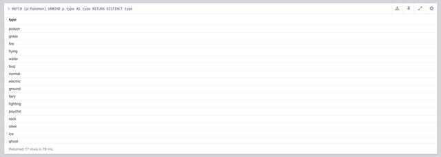
Figure 7-13. The results of a query to get a unique list of all the Pokémon types
With that query, we find that there are 17 types returned, and Trainer 919 only has 16, so we know there’s one missing. There should technically be 18 types, there is one missing, which is the `dark` type. It is not included in the list because it wasn’t introduced until the second generation, and therefore none of the first 151 Pokémon are `dark`.
From Figure 7-12, we know that `steel`, `ghost`, and `fairy` are the top 3 lowest counts, at 1 each. We can use this information to recommend some Pokémon with those types. To do this, it requires the combination of the previous query, and some additional Cypher code, which looks like so:
MATCH (t:Trainer)-[]-(p:Pokemon)
WHERE id(t) = 919
UNWIND p.type AS type
WITH type, count(type) AS total, t
ORDER BY total ASC
LIMIT 3

MATCH (p:Pokemon)
WHERE type IN p.type
AND NOT (t)--(p)
RETURN p.name, p.type
LIMIT 5
The first part of the query is the exact one from before, just with a WITH clause in place of RETURN. The values passed over by WITH have already been evaluated, so type is being iterated over, and counted. With the use of WITH, each of the types from the previous query can be used in WHERE. Since the types are stored in an array, they must be filtered using IN, as you cannot compare two arrays. This essentially means to compare two arrays, you must be first iterating over the first, then use IN to check if the value is in the second.
In this case, the query is checking to see if one of the top 3 types (`steel`, `ghost`, and `fairy`) are within a Pokémon’s type array. There’s nothing worse than being recommended something that you already have, and the same goes here. To get around this, AND is used to add that the Trainer cannot be related to the Pokémon returned. Gotta catch em’ all, right? To stop too many choices being returned, the results are limited, after the `name` and `type` are returned. The results of the query can be seen in Figure 7-14.
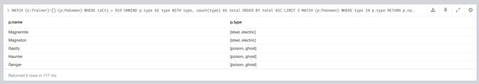
Figure 7-14. The top 5 results for Pokémon with the least popular types that Trainer 191 had
This data can be incredibly useful for Trainer 919 to help them catch some Pokémon that round out their types a little better. If this information was fed back into the Pokémon website, it should easily recommend these Pokémon as good suggestions to catch. The ordering of the query could also be reversed to show a list of Pokémon that should be caught to add to the more popular types owned, which would help if you were trying to get all Pokémon of a certain type, for example.
If you’re attempting any kind of collection, it’s always nice to have an idea of how much is remaining, and a Pokémon Trailer is no different. It’s always handy to have a list of the renamed Pokémon you had to catch, and luckily Cypher can help with that using the following simple query.
MATCH (p:Pokemon), (t:Trainer)
WHERE id(t) = 919
AND NOT (t)--(p)
RETURN p.name
Once again we use Trainer 919 as an example by using the combination of WHERE and the id function. We’re also matching Pokémon (`p`), but without any matches this time. Essentially what’s being done here is any Pokémon that aren’t related to Trainer 919 are then returned, and we have our list of remaining Pokémon. The results for this query can be seen in Figure 7-15.
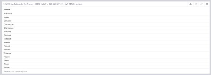
Figure 7-15. The remaining Pokémon Trainer 919 has to catch
Relating to e-Commerce
Some of the queries used for the Pokémon examples can also be applied to an e-commerce application for recommending products, instead of Pokémon. We’ll go through a couple of these applications to show how the same query can be used to achieve a similar result.
Most Popular Product
Knowing which product is the most popular in your store is always going to be a good thing. We’ve already calculated the most popular Pokémon caught by Trainers, which is essentially customers buying products. In an e-commerce based structure, products would be somehow related to customers, either directly, or through orders. This link allows you to query the dataset for any products that have a customer or order connection, and then count those. This will give stats on the most popular products, which could then be broken down by category. Assuming that orders were related to products in some way, an example Cypher query would look like so:
MATCH (p:Product)--(:Order)
RETURN p.name AS name, count(p.name) AS count
ORDER BY count DESC
LIMIT 15
Since a product is related to an order, provided the relationship exists, it has been bought. With this match in place, it’s just a case of returning the product name, with a count of the products, and finally ordering by that count, in descending order. This particular query has a limit of 15, but this could easily be changed to say 1, to only return the top product.
This same logic, applied on a per-customer basis, would allow you to see which products your customers bought most often. You could then take these products, and promote deals containing them, or the products themselves to the customer, because you know these are deals they’ll be interested in. Assuming the same structure as before, but with the addition of a customer being related to an order, an example Cypher query would be like so:
MATCH (p:Product)--(:Order)--(c:Customer)
WHERE id(c) = 919
RETURN p.name AS name, count(p.name) AS count
ORDER BY count DESC
LIMIT 15
The same query as before now adds another relationship to the match, in the form of a `Customer` node. When a customer makes an order, their node will be related to an order node, which will be related to product nodes. This gives the customer a link to the products, which query takes advantage of using a WHERE to filter the results. This gives the customer the most purchased products, and can be then used to promote any deals containing those products.
Most Popular Product Category
A customer may buy a whole range of products, but only ever buy each one once. If you were to try to work out their most popular product, there wouldn’t be much information to go on. The products themselves though will be part of a category, and it may be that this customer likes a particular category. Depending on how the categories have been set up, it may be that each product has an array of categories, much like our Pokémon nodes and their types. The same query used for getting the most popular type can also be used here for the most popular category. However, the more likely case will be that products are related to categories via Category nodes, which would contain many products.
If the categories are related as nodes, then it then means you can access a customer’s favorite category through the products they’ve bought. This can be achieved building on the query used in the previous example, and would look something like this:
MATCH (c:Category)--(:Product)--(:Order)--(u:Customer)
WHERE id(u) = 919
RETURN c.name AS name, count(c.name) AS count
ORDER BY count DESC
LIMIT 15
The query adds another relationship to the MATCH clause, including the Category nodes that are related the purchased products of the customer. In this case, the WHERE and the customer relationship could be removed, which would give an overall view on the most popular products within the whole store.
Just as we recommended Pokémon to Trainers earlier, it’s just as easy to recommend products to customers. Depending on your use case, you may want to recommend a customer’s most popular product to them or just those in the same category. In the case of the category, there isn’t too much that needs to be added to the previous query, used to get the top categories. All that’s required is to get the products related to the linked categories, which would look something like this:
MATCH (p:Product)--(c:Category)--(:Product)--(o:Order)--(u:Customer)
WHERE id(u) = 919
AND NOT (o)--(p)
RETURN p.name AS name
The query gets the products from the related categories, but in the AND, also checks to make sure the product and order nodes are not related, as this would mean the products have been purchased before. Of course, this would just return products in the same category, but there may be other values available to make the query more accurate, and therefore give more targeted results.
Thank You
Before moving on, I have to thank all of those who participated in the Pokémon website, and submitted their data to be used in the book. I may never meet any of the users who submitted data to the website, but I can at least thank each and every person for submitting their data and helping make this chapter. As I mentioned earlier, I wanted to make this chapter a little different, and thanks to the community that has happened.
The project itself will be available on GitHub when the book is published (with the data removed, of course) so anyone can look at the code. As the url isn’t known yet, if you’re interested in seeing the project, just check my github account, chrisdkemper and look for it there.
Out of the box, Neo4j doesn’t handle location-based queries, but with the addition of a plugin, that can easily be changed. The plugin in question here is the Neo4j Spatial plugin (https://github.com/neo4j-contrib/spatial) which adds location-based functionality to Neo4j. Although we won’t be detailing all of the functionality included in the plugin here, if you’d like to find out more then have a look at the github page.
To do these queries there are a couple of steps you need to take to allow for the data to be used. For now though, these steps won’t be covered (as they will be in the next chapter) so these queries assume you’ve got the spatial plugin setup for them to work.
For now we need an example. Where I live, Newcastle, UK, there is a local rail system called the Metro. I’ve gathered the location data for these rail lines so it can be used in the examples. Within the region there are 60 stations, so for these examples it’ll be using various random points within the city, and around the stations in question. This should give an idea on how to perform the queries needed to return nodes based on location, that can be adapted to your own application.
Figure 7-16 shows how the data looks in the browser if you run MATCH (n) RETURN n on the Metro station database, with the spatial database set up.
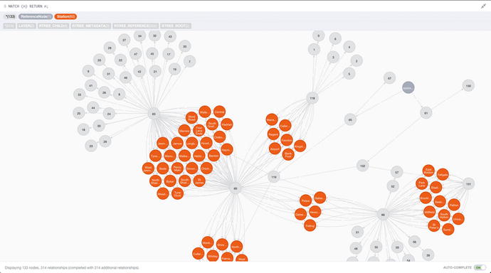
Figure 7-16. The result of running MATCH (n) RETURN n; on a database location data set up on the spatial plugin
You can see the stations with various relationships linking groups of stations. You’ll have to take my word for the fact that the areas that have the most relationships are where the stations are the closest together. This helps give an idea of how the spatial plugin works. With that out of the way, let’s look at some queries, starting with where the closest Metro station is.
If you’re in a strange place, being able to find the closest mode of transport could always be useful, so we’ll do that here, just with Metro stations. The cypher needed to achieve this query isn’t too complicated, we just need a location and a distance. The distance needed is in kilometers, and a location to start from is provided. When this is queried in Cypher, it’s looked up via the plugin and the results are returned, and can be used as needed in your application. In this case, the query is where the nearest Metro station is. The query needed to run this query is as follows:
START n=node:geom("withinDistance:[54.9773781,-1.6123878,10.0]") RETURN n LIMIT 1
The location being used here is one near City Hall. If you run this query the result can be seen in Figure 7-17. The query itself is using START to initiate a traversal of the graph. It then uses the geom index to perform the function, which has arguments of latitude, longitude, and distance (in kilometers) respectively.

Figure 7-17. The result of performing the distance query for a given location on Metro station data
You’ll just have to take my word on the fact that the query is correct as Haymarket is in fact the closest Metro station to that location at City Hall. This shows how easy it is to query located data, so with a bit of setup (which will be covered in the next chapter), you’ll be able to have location awareness in your applications.
Summary
Through the course of the chapter, a large spectrum of different query types have been shown and demonstrated, using (hopefully) interesting means. There’s been many different types of recommendation and analysis queries from the Pokémon website, and the closest location query made possible by the spatial plugin. These varying uses will hopefully be useful enough to help push you in the right direction when it comes to your own applications. Now though, it’s time to build an application that takes everything we’ve done so far in the book and puts it all together.