Chapter 2. Online Streaming Experiment
Digital A/B tests such as AirCnC’s 1-click button are the simplest and easiest to implement, so we’ll first see how to do one from A to Z. This doesn’t mean that there aren’t opportunities to mess it up and end up with a useless experiment, so we’ll have to be careful! Making your experiment a success starts much before any customer or employee sees your treatment.
In the first section, we’ll review carefully how to plan the experiment, which involves understanding what you’re testing as well as your criteria for success and what makes you believe your experiment will be a success.
In the second section, we’ll then determine our sample size, the number of customers (experimental psychologists would say “subjects”) we need to include in our experiment, as well as the “statistical power” of our experiment. In this section, I’ll do a deep dive into the meaning of statistical significance and I’ll show you how to use simulations instead of traditional statistics. That material will be heavier than usual, as I’ll introduce a number of concepts and methods that we’ll reuse for the other experiments, but if you stick around, I promise that you’ll never have to worry or puzzle over p-values ever again.
Finally, in the third section, we’ll analyze our experimental data, using a traditional test of proportions and then a logistic regression.
Planning the experiment
Planning is a crucial step of experimental design. Experiments can fail for a variety of reasons many of which you can’t control, such as the implementation going awry; but poor planning is both a frequent cause of failure and one you can control.
To make it easy to digest and remember, I’ll break down this phase into three steps:
-
Criteria for success
-
Definition of intervention
-
Logic for success
Criteria for success
You might be surprised that I start with the criteria for success instead of the definition of the intervention. After all, shouldn’t we know what we’re testing first? Unfortunately, a common cause of failure is the decision to test something (often the latest management fad or something that your boss’s boss read about) without a clear sense of what we’re solving for.
What does success look like? Ideally, it should be expressed in terms of dollars of additional revenue or decreased cost. If that’s not possible, you should at least have an operational metric that seems reasonably connected to business outcomes. In the case of the 1-click button, we can obviously look at booking rates. But what about the duration of website visit? If the button shortens how long it takes someone to book a trip but otherwise doesn’t increase bookings in any way, is that a success or not? What about satisfaction with the booking experience and net promoter score? These may not translate directly into dollar figures, but it is reasonable to assume that improving them has a positive impact for your business.
A compromise you’ll often have to make at this point is to use “leading indicators”—basically causes of the variables you’re ultimately interested in. For example, sign-up can be used as a leading indicator for usage, usage for amount purchased, etc. This will allow you to report results much earlier than if you used long-term business metrics. You may care about your customers’ LTV (Life-Time Value, the total amount they’ll spend with your company) but have to settle for 3-month booking amount.
This is sometimes done informally, by picking operational metrics as targets for experimentation and assuming with some hand-waving that these will end up benefiting the company’s bottom line. Of course, armed with this book, we can do better. We can validate and measure the causal connection between a short-term operational metric and long-term business outcomes through an observational study or a dedicated experiment, as we’ll see later.
Here again, the goal is to make good business decisions. I don’t want to be a fanatic of dollar figures, because it would be unduly restrictive and would exclude a large range of business improvements. At the same time, you want to make sure that you have a measurable target metric that you’ll be able to track. There are several potential pitfalls that you should avoid here.
The first one is picking something you can’t measure reliably. What would it mean to say “the 1-click button makes the booking experience easier”? How would you measure it? Asking the product manager or the product owner to decide after the fact whether there has been an improvement is not a measurement. “Our customers rate the website as easier to navigate, as measured by a 2-question survey at the end of a visit” may be an imperfect proxy but at least it can be measured.
The second pitfall is to write down a laundry list of metrics, such as “success would be an improvement in booking rate, booking amount, customer satisfaction or net promoter score”, or even worse, to wait until after seeing the results to determine the metrics for success—e.g. you were originally thinking that the experiment would improve customer experience, but when the results come, customer experience is flat and average website session duration has improved. The problem with that approach is that it increases the risk of false positives (calling the result a success when it was a random fluke)1. It’s ok however to have up to 2 or 3 target metrics that are clearly defined before the experiment as long as you take that into account when analyzing the results (more on that later).
Definition of intervention
Once we have our criteria for success, we can work on defining our intervention. You may remember our earlier discussion of customer satisfaction in chapter 5, and how many rather hidden assumptions were going into a CSAT score. The same problem occurs here: there can be a large gap between a business idea, so used and familiar that everyone immediately feels they know what it is, and a specific implementation.
On the face of it, what could be simpler than a “1-click booking” button? Most of us have seen it implemented on the website of an online retailer and the idea seems perfectly straightforward. But if you think about the nitty-gritty details of how it would be implemented, there are actually a lot of questions to answer, each with multiple possible answers:
-
At which point in the process does the button become available?
-
Where is the button located?
-
What does the button look like? Is it in the same colors as the other buttons on the page or does it stand out in a bright and rich color?
-
What is written on the button?
-
What information do we need about a customer to make 1-click booking available and how do we make sure we have it?
-
What happens after the customer clicks the button? What page are they taken to, and what, if any, actions do they still have to take?
-
Etc., etc.
Let’s say for example that the website’s color theme is pastel green and blue, to hint at nature and travel, and the new button is a shiny red. If that button increases booking, it might be because of the attractiveness of 1-click booking, but it could also be because customers otherwise struggle to see the normal booking button and give up. In that case, the cause of the increase in booking is really “a more visible booking button” rather than “a 1-click booking button”, but you can’t distinguish between the two because the 1-click button was also more visible. Unfortunately, you can’t ever just test one idea, as you’re always also testing the many ways in which it is implemented.
The lesson here is that A/B testing is a powerful but narrow tool. You need to be careful not to make—or let others make—grand statements about what a specific experiment says. It is definitely easier said than done, because business partners often want answers that are broad, clear cut and without fine prints. With that said, even simply stating in your presentation that you’re testing a specific implementation and not a general idea can be useful, for example “this experiment will test the impact of a 1-click button under such and such conditions, and its results should not be interpreted as applying to booking buttons more broadly”.
A better yet alternative would be to test different implementations of the same concept in the experiment. If four slightly different 1-click button treatments have the same impact, you can more confidently draw conclusions regarding the general impact of 1-click booking; on the other hands, if they have very different impacts, then this suggests that implementation matters a lot and that you need to be very careful with your conclusions regarding how a specific implementation will generalize.
Logic for success
Once we know our criteria for success and we have defined our intervention, the last step is to connect the two through the logic for success: why and how would our intervention impact our criteria for success?
This is another surprisingly common source of failure for experiments: a problem has been identified and someone decides to implement the latest management fad that they have been thinking about recently, even though it’s unclear why it would help with this specific problem. Or someone decides that a more attractive and simpler User Interface will increase purchase amounts. To have confidence in our experiment, you need to be able to articulate a reasonable behavioral story2. In the case of 1-click booking, you might hypothesize that customers identify an attractive booking but give up before completing their booking because the booking process is cumbersome; the 1-click button would impact the probability of booking by shortening and simplifying the booking process. Drawing a CD here comes handy to visualize your logic (figure 8-1).
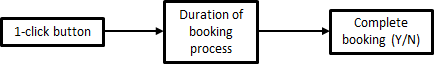
Figure 2-1. Articulating our logic for success with a CD
Overall, articulating your logic for success has two benefits.
First, it is often testable in itself. Does a large number of customers actually drop off between starting a booking and completing it? If so, the hypothesized logic makes sense from a behavioral data perspective. But if, for example, most customers leave without having started the booking process with a specific product, e.g. because they couldn’t find something that appealed to them or they were overwhelmed with the number of options, then AirCnC is trying to solve the wrong problem; it’s unlikely that offering 1-click booking will improve their numbers.
Ask yourself: what would confirm or infirm our logic? What would the data look like if it were true or false? If you don’t have the necessary data at hand, it might be worth running a preliminary test, such as bringing in 10 people for User Experience testing—e.g. observing them trying to use your website while they’re thinking out loud. This may not fully confirm or infirm your logic, but it will probably give you some indication, at a fraction of the development cost for the solution considered. As the often-cited quote by Albert Einstein goes, “If I had an hour to solve a problem, I’d spend 55 minutes thinking about the problem and 5 minutes thinking about solutions”.
The second benefit of articulating the logic of your intervention is that it will generally give you a sense of the potential upside. What would the numbers look like, in the best-case scenario, if the problem at hand was solved? Assuming that all customers who drop off during the booking process would complete it with 1-click booking, how much would the booking rate increase? This is the best-case scenario from the perspective of the experiment because we’re assuming that it would fully solve the problem, which is unlikely in reality. If the increase in booking rate under this scenario would not pay for the implementation of the 1-click booking, then don’t even bother testing it.
Once you’ve validated that your best-case scenario would be profitable, you can start thinking about your most likely scenario. How much would we expect 1-click booking to improve the booking rate? There is undoubtedly a lot of subjectivity and uncertainty involved, but it can still be a worthwhile exercise, by making explicit people’s assumptions and gut feelings. Use your business sense and understanding of the processes. If most customers are dropping off at the exact same step in the process, e.g. payment, then it’s likely that there is something wrong with that specific step—people don’t all run out of patience at the exact same time. You can then compare the expected benefits with the cost of implementing the solution. Is it still worthwhile?
You can also approach this question from the other side: start by determining the break-even point of the solution, i.e. the improvement in the target metric that would make the solution profitable to implement, and then consider whether that improvement is realistic from a behavioral standpoint. From a psychological perspective, it’s better to start with the expected result than with the break-even point: if you start with the break-even point, you’re more likely to anchor on it and find reasons to justify that it’s achievable. However, in many cases, you’ll know the break-even point first, for example if it was calculated during a preliminary cost-benefit analysis; your company or business partners might also request it and refuse to think about the expected result first. Don’t worry too much about it. Regardless of whether you’re working with your expected or best-case result, we’ll need it to determine the minimum detectable effect for our experiment.
It’s important that your logic connects your proposed solution with your target metric. Don’t leave it to “this will improve the customer experience”. How will you know it? If your logic is solid, you should be able to express it in terms of a causal diagram, with at least some of the effects being observable.
A useful rule of thumb to help you articulate your logic is to break down your business metric into components. For example, revenue (or most of its variations) can be broken down into number of customers, probability/frequency of purchase, quantity purchased, and price paid. Determining which components are likely to be affected can allow you to better articulate the business case. If your business partners are concerned by a decrease in the number of customers and the proposed intervention would most likely only increase the quantity purchased, you need to clarify with them that they would still call it a win. This approach can also reduce the noise in your experiment; if the proposed intervention would most likely only increase the quantity purchased, you can focus on that metric and disregard somewhat random fluctuations in price paid.
Determining random assignment and sample size/power
The next phase is determining how we’ll assign customers randomly to our two experimental groups, control and treatment, as well as how many customers we need to include in our experiment.
Random assignment
The theory of random assignment could not be simpler: whenever a customer reaches the relevant page, they should be shown the current version of the page (called “control” in experimental jargon) with a 50% chance and the version with the 1-click booking button (the “treatment”) with a 50% chance.
From a coding perspective, assuming that you are not using a software that takes care of it for you, this can easily be implemented in R or Python:
-
Whenever a new customer reaches the relevant page, we generate a random number between 0 and 1;
-
Then we assign the customer a group based on that random number: if K is the number of groups we want (including a control group), then all individuals with a random number less than 1/K are assigned to the first group; all individuals with a random number between 1/K and 2/K are assigned to the second group, and so on.
Here, K is equal to two, which translates into a very simple formula:
## R>K<-2>assgnt=runif(1,0,1)>group=ifelse(assgnt<=1/K,“control”,“treatment”)## PythonK=2assgnt=np.random.uniform(0,1,1)group="control"ifassgnt<=1/Kelse"treatment"
There are, however, a certain number of subtleties which can trip novice experimenters.
The first one is determining the right point in time for random assignment. Let’s say that whenever a customer gets on the first page of the website, you assign them to either the control or the treatment group. Many of these customers will never reach the point of making a booking and will therefore not see your booking interface. This would dramatically reduce the effectiveness of your experiment because you would in effect experiment only on a fraction of your sample.
When determining which customers should be part of the experiment and when they should be assigned to an experimental group, you should reflect on how the treatment will be implemented if the experiment is a success. Your experimental design should include the same people who would see the treatment if it got implemented in business as usual and only them. Visitors who leave the website before booking will still not see the button, whereas any future promotion or change to the booking page would be built in addition so to speak “on top of” the button which would always be present. Therefore, non-booking visitors should be excluded but customers with a promotion should be included.
The second challenge is making sure that the random assignment is happening at the “right” behavioral level. I’ll explain what this means with an example. Let’s say that a visitor comes on the AirCnC website, starts a booking but then for whatever reason leaves the website (they got disconnected, it’s time for dinner, etc.) and comes back to it later. Should they see the same booking page? If they were offered 1-click booking the first time, should they still be offered it the second time?
The problem here is that there are really multiple levels that could potentially make sense. You could assign control or treatment at the level of a single website visit, of a booking, however many visits it takes, or at the level of a customer account (which may or may not be the same person if several people in a household use the same account). Unfortunately, there are no hard rules here, the right approach must be determined on a case-by-case basis by thinking about the conclusions you want to draw and what a permanent implementation would look like.
In many cases, it makes sense to do an assignment at the closest level you can to a human being: customer account if you can’t distinguish people in a household, or individual customer if they each have a sub-account, as is the case for example with Netflix. Human beings have persistent memories and alternating options for the same person can get confusing. Here, this would mean that our AirCnC customer should see the 1-click button for the whole duration of the experiment, regardless of how many visits and bookings they make during that time. Unfortunately, this means that you can’t just roll the dice metaphorically each time someone starts a booking on the website to determine their assignment; you need to keep track of whether they have been assigned in the past and if so to which group. For a website experiment, this can be done through cookies (assuming the customer allows them!).
Warning
The level at which you’re making your random assignment should also be the level at which you calculate your sample size. If you make assignments at the customer level and customers make an average of 3 visits per month, you’ll need a 3x longer experiment than if you make assignments at the visit level. But the level you choose for your random assignment should determine your sample size, not the other way around!
Whatever level you choose, you’ll have to keep track of the assignment(s) to be able to link them to business outcomes later. This is why best-in-class companies use centralized systems that record all assignments and connect them to customer IDs in a database, so that they can serve a consistent experience to customers over time.
More broadly, what these two challenges point at is that the implementation of a business experiment is almost always a complex technical affair. A variety of vendors now offer somewhat plug-and-play solutions that hide the complexity under the hood, especially for website experimentation. Whether you rely on them or on your internal tech people, you’ll need to understand how they’re doing the random assignment to make sure that you’re getting the experiment you want.
A good way to check that the system works correctly is to start with an A/A test, where there is a random assignment but the two groups see the same version of the page. This will allow you to check that there are indeed the same number of people in the two groups and that they don’t differ in any significant way.
Sample size and experiment power
Once we know what we’re going to test and how, we need to determine our sample size. In some cases, as here with our 1-click booking experiment, we can choose our sample size: we can just decide how long we want to run the experiment. In other cases, our sample size might be defined for us. If we’re going to run a test across our whole customer or employee population, we can’t increase that population just for the sake of experimentation!
Regardless of the situation we’re in, we will look at our sample size in relation to other experimental variables, such as statistical significance, and not in a vacuum. Understanding how these variables are related is crucial to ensure that our experimental results are usable and that we’re drawing the right conclusions from them. Unfortunately, these are highly complex and nuanced statistical concepts and they have not been developed for business decisions.
In line with the spirit of this book, I’ll do my best to explain these statistical concepts and conventions in the context of business decisions. I’ll then share my reservations about the traditional conventions and offer my two cents regarding how to tweak them while remaining in the traditional framework. And finally, I’ll describe an alternative approach that has been slowly gaining momentum and which I think is superior, namely using computer simulations.
A little bit of statistics theory without math
When running an experiment such as the “1-click booking” button, our goal is to make the right decision: should we implement it or not? Unfortunately, even after running an experiment (or a hundred), we can never be 100% sure that we’re making the right decision, because we have only partial information. Certainly, if we ran an experiment for years on end, we might reach a point where there is only 1 chance in a million that we’re wrong, but lotteries often have worse odds and people still win. Moreover, we generally don’t want to run an experiment for years on end, when we could be running other experiments instead! Therefore, there’s a trade-off between the sample size of an experiment and our degree of certainty.
Because we can never know after the fact whether a specific decision was right or not, our approach will be to try to select a good sample size and a good decision rule before the experiment. What does “good” mean here? Well, the very best possible sample size and rule would be those that maximize our expected profit over time. The corresponding calculations are doable but require advanced methods that are beyond the scope of this book3. Instead, we’ll rely on the following measures:
-
Assuming that our 1-click button does increase our booking rate, what is the probability that we’ll rightly implement the button? This is called the “True Positive” probability. On the other hand, if there is a positive effect and we wrongly conclude that there is none, it’s called a “False Negative”.
-
Assuming that our 1-click button has no discernible effect (or, God forbid, a negative effect!) on our booking rate, what is the probability that we’ll wrongly implement the button? This probability is called the “False Positive” probability. On the other hand, if there is no effect and we rightly conclude that there is no effect, it’s called a “True Negative”.
These various configurations are summarized in table 8-1.
| Do we implement the 1-click booking button? | |||
| YES | NO | ||
| Does the 1-click booking button increase the booking rate? | YES | True Positive | False Negative |
| NO | False Positive | True Negative | |
Table 8-1. Making the right decision in the right situation
We would want our True Positive and our True Negative rates to be as high as possible, and our False Positive and False Negative rates to be as low as possible. However, the simplicity of this table is deceptive, and it actually encompasses an infinite number of situations: when we say that the button increases the booking rate, it could mean that the increase is 1%, 2%, etc. On the other hand, when we say that the button does not increase the booking rate, it could mean that it has exactly zero effect, or that it is decreasing the booking rate by 1%, 2%, etc. All these effect sizes would have to be factored in to calculate the overall True Positive and True Negative rates, which would be too complicated. Instead, we will rely on two threshold values.
The first one is an impact of exactly zero for all subjects, also called the “sharp null hypothesis” (the non-sharp “null hypothesis” would be an average zero effect across subjects). The False Positive rate for this value is called the statistical significance of our experiment. Because a negative impact would be easier to catch than a null effect, the False Positive rate for any negative value will be at least as large as the statistical significance, and larger negative effects will have higher False Positive rates. The most common convention in academic research is to set the statistical significance at 5%, although in certain fields such as particle physics, it can sometimes be as low as 0.00000054.
The second threshold value is set at some positive effect that we’re interested in measuring. For example, we might say that we want to choose a sample size so that we can be “reasonably sure” that we will capture a 1% increase in booking rate, but we’re okay with missing smaller effects than that. This value is often called the “alternative hypothesis”, and the True Positive rate for this value is called the statistical power of our experiment. Because larger effects would be easier to catch, the True Positive rate for any larger value will be at least as large as the statistical power, and larger positive effects will have higher True Positive rates. “Reasonably sure” is traditionally taken to mean 80%.
Our table updated according to the traditional convention would therefore look like table 8-2.
| Do we implement the 1-click booking button? | ||
|---|---|---|
| YES | NO | |
| The 1-click booking button increases the booking rate by more than 1% | >80% (larger for larger effect sizes) | <20% (smaller for larger effect sizes) |
| The 1-click booking button increases the booking rate by exactly 1% | 80% (statistical power) | 20% (1-statistical power) |
| The 1-click booking button increases the booking rate by less than 1% | <80% (larger for larger effect sizes) | >20% (smaller for larger effect sizes) |
| The 1-click booking button has exactly no impact on the booking rate | 5% (statistical significance) | 95% (1-statistical significance) |
| The 1-click booking button strictly decreases the booking rate | <5% (smaller for larger negative effect sizes) | >95% (larger for larger negative effect sizes) |
Table 8-2. The thresholds used in the traditional statistical approach
Setting your experiments to have a power of 80% for the effect size of interest means that, on average, 20% of your experiments with a valuable effect of the intervention will wrongly reject the intervention. In my opinion, what is the point of designing good and good valuable interventions if you’re going to reject them? I would therefore target a statistical power of 90% for our effect of interest of 1%.
Regarding statistical significance, the conventional approach introduces a fixed asymmetry between the control and the treatment with a statistical significance threshold of 95%. The bar of evidence the treatment has to pass to get implemented is much higher than for the control, which is implemented by default. Let’s say that you’re setting up a new marketing email campaign and you have two options to test. Why should one version be given the benefit of the doubt over the other? On the other hand, if you have a campaign that has been running for years and for which you have run hundreds of tests, the current version is probably extremely good and a 5% chance of wrongly abandoning it might be too high; the right threshold here might be 99% instead of 95%. More broadly, relying on a conventional value that is the same for all experiments feels to me like a missed opportunity to reflect on the respective costs of false positives and false negatives. In the case of the 1-click button, which is easily reversible and has minimal costs of implementation, I would target a statistical significance threshold of 90% as well.
To recap, from a statistical perspective, our experiment can be summarized by 4 values:
-
The statistical significance, often represented by the Greek letter beta (β);
-
The Effect size chosen for the alternative hypothesis;
-
The statistical power, often represented as 1- α where α is the False Negative rate for the chosen alternative effect size;
-
The sample size of our experiment, represented by N.
These four variables are referred to as the B.E.A.N. (Beta, Effect size, Alpha, sample size N), and determining them for an experiment is called a “power analysis”5. For our 1-click button experiment, we have decided on the first 3 of them and we only have to determine the sample size. We’ll see next how to do it with traditional statistical formulas and then how to do it with computer simulations.
Traditional power analysis
The appropriate statistical test here would be a Test of Proportions, because our target variable is binary (Complete booking Y/N) and we’ll compare the proportions of customers completing a booking in our two experimental groups. As it is a standard test, the formula to calculate the corresponding sample size is easily available. In R, we’ll use the pwr package.
With an average booking rate of 17% in our historical data, the chosen effect size of 1% would translate into an expected booking rate for our treatment group of 18%. For the standard values of the parameters—statistical significance = 0.05 and power = 0.8—the corresponding formula in R would be:
## R>library(pwr)>effect_size<-ES.h(0.194,0.184)>pwr.2p.test(h=effect_size,n=NULL,sig.level=0.05,power=0.8,alternative="greater")Differenceofproportionpowercalculationforbinomialdistribution(arcsinetransformation)h=0.02554423n=18950.14sig.level=0.05power=0.8alternative=greaterNOTE:samesamplesizes
The syntax of all the functions for power analysis in the pwr package is the same, with the exception of the notation for the effect size, which changes from one formula to another:
-
h is the effect size, based on the increase in probability we want to be able to observe over the baseline probability;
-
n is the sample size for each group;
-
sig.level is the statistical significance;
-
power is the statistical power, equal to 1-α.
When entering the formula, you should enter the values for three of these variables and set the remaining one to NULL. In the formula above, we’re calculating the sample size, so we set n = NULL.
Note that for a test of two proportions, the effect size for statistical purposes depends on the baseline rate; an increase of 5% from a baseline of 10% or 90% is more “important” than from a baseline of 50%. Fortunately, the package pwr provides the ES.h function which translates the expected probability and the baseline probability into the right effect size for the formula.
Note also the parameter at the end of the formula: alternative indicates whether you want to run a 1-sided (“greater” or “less”) or a 2-sided (“two.sided”) test. As long as our treatment doesn’t increase our booking rate, we don’t really care whether it has the same booking rate or a lower booking rate compared to our control; either way, we won’t implement it. This implies we can run a one-sided test instead of a two-sided test by setting “alternative = ‘greater’”.
The code for Python is similar, but we need to calculate our standardized effect size ourselves, by plugging the formula from the ES.h function in the R library pwr.
## Pythonfrommathimportasin,sqrtimportstatsmodels.stats.powerassspeffect_size=2*asin(sqrt(0.194))-2*asin(sqrt(0.184))ssp.tt_ind_solve_power(effect_size=effect_size,alpha=0.05,nobs1=None,alternative='larger',power=0.8)Out[1]:18950.818821558503
The sample size returned by the formula is 18,950 per group (plus or minus some minor variation between R and Python), i.e. 37,900 total, which means we can achieve the necessary sample size in a bit less than 4 months. That was easy! Using a statistical significance of 0.1 and a power of 0.9 would yield a sample size of 20,136 per group, just a bit longer.
However, these sample sizes are calculated for a statistical test of proportions, not a regression. Such statistical tests are very simple but do not allow for the inclusion of other predictors or other methods such as matching to reduce noise. In addition, they rely on statistical assumptions regarding your data that may or may not be valid. Formulas for linear regression exist, but they still rely on statistical assumptions, and there is no formula for logistic regression. Therefore, we’ll use a general approach instead that doesn’t rely on any assumption regarding your data: simulations.
Power analysis without statistics: simulations
The logic of using simulations is very simple: we’re going to use some of our past historical data to “fake” an experiment and see what happens. By running a large number of such fake experiments, we can get a reasonable idea of what will happen in our real experiment under a variety of situations. What if the button has no effect whatsoever? What if it increases the booking rate by 1%? By 10%? What if we run the experiment with 10,000 customers? 40,000? Simulations will tell you!
Simulations at scale can be a little difficult to wrap your head around, so I’ll start with single runs that demonstrate how we can simulate false positives, and then false negatives.
Understanding simulations: false positives
First, we’ll tackle false positives, because they’re easier to understand. Let’s assume that our 1-click button has no impact on the booking rate. This means that on average our control group and our treatment group should have the same booking rate. The key phrase here is “on average”: if we take 2,000 customers and assign them at random to one of two groups, these two groups are unlikely to have exactly the same booking rate, because of random variations. Think of coins: if we toss two coins 10 times each, we expect that they’ll both have about 5 tails and 5 heads, but one might have 6 and 4, while the other has 3 and 7. Life is random! The question is how random it might get. It is possible that out of sheer luck all customers in one group will book a location and none in the other group does, but that’s extremely unlikely, so we can safely ignore that possibility. But what about a 10% difference? Could one group have a 55% booking rate and the other a 65% booking rate just out of luck? That’s where simulations come in.
We have a bit less than 3 years of historical data, and we know with certainty that the button could not affect them, because it was not in place. This is how we’ll proceed:
-
Draw at random 2,000 observations from our data;
-
For each one of them, change the OneClick variable to 1 with probability 50% (i.e. we randomly assign them to the treatment group);
-
Run a regression and measure the coefficient and p-value for the OneClick variable.
## R>n<-2000>prob_button<-runif(n)>sim_data<-hist_data%>%+sample_n(K)%>%+mutate(oneclick=ifelse(prob_button>0.5,1,0))>sim_mod<-glm(booked~age+gender+period+oneclick,+family=binomial(link="logit"),data=sim_data)>summary(sim_mod)Call:glm(formula=booked~age+gender+period+oneclick,family=binomial(link="logit"),data=sim_data)DevianceResiduals:Min1QMedian3QMax-2.0298-0.5282-0.2785-0.11163.0201Coefficients:EstimateStd.ErrorzvaluePr(>|z|)(Intercept)10.296240.6645815.493<2e-16***age-0.318150.01834-17.349<2e-16***gendermale0.135190.142580.9480.3430period-0.017310.00713-2.4280.0152*oneclick0.273510.142801.9150.0554.---Signif.codes:0‘***’0.001‘**’0.01‘*’0.05‘.’0.1‘ ’1(Dispersionparameterforbinomialfamilytakentobe1)Nulldeviance:1810.8on1999degreesoffreedomResidualdeviance:1276.6on1995degreesoffreedomAIC:1286.6NumberofFisherScoringiterations:6
As you can see, the coefficient for the OneClick variable is not null, and actually pretty high compared to the coefficient for age (in absolute value). Our imaginary button has about the same effect as decreasing a customer’s age by 1 year! It’s also statistically significant at the 10% threshold and close to the 5% one, with a p-value of 0.055. That’s clearly a false positive, given that we flipped the OneClick variable at random without changing anything else.
The corresponding Python code is
## Python code (output not shown)random.seed(123)np.random.seed(123)# Simulating the experiment with no true effectn=2000prob_button=np.random.uniform(size=n)sim_data_df=hist_data_df.sample(n).drop('oneclick',axis=1)sim_data_df['prob_button']=np.random.uniform(size=n)sim_data_df['oneclick']=sim_data_df['prob_button'].apply(lambdax:1ifx>0.5else0)# Running a logistic regressionimportstatsmodels.formula.apiassmfmodel=smf.logit('booked ~ age + gender + period + oneclick',data=sim_data_df)model.fit().summary()
To determine how large (again, in absolute values) false positives can get, we can repeat the previous process, say 1,000 times and see what happens. The code is the same, except that we save our results in a list that we then convert into a data frame.
## R>#Simulation loop>Nloop<-1000>set.seed(1234)>ptm<-proc.time()>sim_list<-list()>n<-2000>for(iin1:Nloop){+sim_data<-pre_data%>%+sample_n(n)%>%+mutate(oneclick=ifelse(runif(n)>0.5,1,0))+sim_mod<-glm(booked~age+gender+period+oneclick,+family=binomial(link="logit"),data=sim_data)+sim_list[[i]]<-data.frame(+coeff=sim_mod$coefficients['oneclick'],+pvalue=coef(summary(sim_mod))[5,4]+)+}>sim_data_summary<-bind_rows(sim_list)>proc.time()-ptmusersystemelapsed15.520.8916.48>summary(sim_data_summary)coeffpvalueMin.:-0.412403Min.:0.002921stQu.:-0.1006931stQu.:0.24325Median:-0.008339Median:0.47684Mean:-0.004953Mean:0.486873rdQu.:0.0997783rdQu.:0.73260Max.:0.390446Max.:0.99547## Python version (output not shown)nloops=1000sample_sizes=[2000]*nloops#Serialized function with FOR loopdeffalse_positive_repeat_sim(sample_sizes):coeff_vector=[]pvalue_vector=[]forsinsample_sizes:sim_data_df=hist_data_df.sample(s)sim_data_df['prob_button']=np.random.uniform(size=s)sim_data_df['oneclick']=sim_data_df['prob_button'].apply(lambdax:1ifx>0.5else0)model=smf.logit('booked ~ age + gender + period + oneclick',data=sim_data_df)res=model.fit(disp=0)# Extracting the coefficients of interest from the summarycoeff_vector.append(res.params['oneclick'])pvalue_vector.append(res.pvalues['oneclick'])sim_summary_df=pd.DataFrame({'coeff':coeff_vector,'pvalue':pvalue_vector})returnsim_summary_dfsim_summary_df=false_positive_repeat_sim(sample_sizes)sim_summary_df.describe()
The coefficient estimates go from strongly negative to strongly positive, and the p-values are distributed uniformly between 0 and 1. By definition of a p-value when there is no effect, about 10% of the p-values are less than or equal to 0.1. Let’s see how large these estimates are by filtering on p-values and taking the absolute values of the coefficients.
## R>sim_data_summary%>%filter(pvalue<=0.1)%>%mutate(coeff=abs(coeff))%>%summarize(min_eff=min(coeff),max_eff=max(coeff),avg_eff=mean(coeff))min_effmax_effavg_eff10.22677980.41240270.290947## Python (output not shown)deff(c):returnpd.Series([c.abs().min(),c.abs().mean(),c.abs().max()],index=['min_eff','avg_eff','max_eff'])sim_summary_df.loc[sim_summary_df.pvalue<=0.1].apply(f).drop('pvalue',axis=1)
There is a 10% chance that we’ll observe a coefficient that will be between 0.23 and 0.41, with an average of 0.29. Remember that these are coefficient in a logistic regression so they don’t have an immediate interpretation, but we can get a sense of their relative size by comparing with the coefficients for the other variables in the earlier regression: at 0.41, our button would have the biggest impact of all variables!
2,000 customers is not that many. What if we run the previous simulation with 10,000 of them, about a month worth of data? The code is identical so I will only provide the results: coefficients in the top 10% are now between 0.105 and 0.23, with an average of 0.13. By using a larger sample, we’ve reduced the random variation in our data and we’re now much less likely to see a large effect out of randomness. As you try out various sample sizes, you’ll get a sense of how much uncertainty you can expect in your real experiment.
Understanding simulations: false negatives
Handling false negatives (falsely concluding that there is no impact when there is one) is more complicated because it depends on the effect size we’re looking at, which we’ve set at 1%.
Dealing with logistic regression also adds some complexity because we don’t observe directly the booking probability, only whether someone booked or not. There are several ways to manage that, with various degrees of complexity and accuracy. The approach I’ll use is somewhat in the middle of the pack in both regards (the steps that are different from the statistical significance simulation are in italics):
-
Calculate the probability of booking in our complete historical dataset;
-
Draw at random 10,000 observations from our data;
-
For each one of them, change the OneClick variable to 1 with probability 50% (i.e. we randomly assign them to the treatment group);
-
For those in the treatment group, increase the probability of booking by 1%;
-
For all observations, reassign the Booked variable based on the probability of booking (e.g. if the probability of booking is 0.5 for an observation, then assign it the value 1 with probability 50%, regardless of the true value)
-
Run a regression and measure the coefficient and p-value for the OneClick variable.
-
Repeat the process 1,000 times.
This approach preserves the observed existing statistical relationships between all of our variables while allowing us to increase the probability of booking in the treatment group. An alternative approach would be to switch 1% of the Booking values in the treatment group from 0 to 1. That second approach is simpler but less precise, so you should simulate a much larger number of “experiments” if you’re using it.
## R>#Add predicted probability of booking to historical data>hist_mod<-glm(booked~age+gender+period,family=binomial(link="logit"),data=pre_data)>pre_data<-pre_data%>%mutate(pred_prob_bkg=hist_mod$fitted.values)>>#Simulation loop>Nloop<-1000>set.seed(1234)>ptm<-proc.time()>sim_list<-list()>K<-10000>>for(iin1:Nloop){sim_data<-pre_data%>%sample_n(K)%>%select(-oneclick)%>%mutate(oneclick=ifelse(runif(K)>0.5,1,0))%>%mutate(pred_prob_bkg=ifelse(oneclick==1,pred_prob_bkg+0.01,pred_prob_bkg))%>%mutate(booked=ifelse(pred_prob_bkg>=runif(K,0,1),1,0))sim_mod<-glm(booked~age+gender+period+oneclick,family=binomial(link="logit"),data=sim_data)sim_list[[i]]<-data.frame(coeff=sim_mod$coefficients['oneclick'],pvalue=coef(summary(sim_mod))[5,4])}>sim_data_summary<-bind_rows(sim_list)>proc.time()-ptmusersystemelapsed48.610.1848.93>summary(sim_data_summary)coeffpvalueMin.:-0.15894Min.:0.00000661stQu.:0.056461stQu.:0.0333601Median:0.09374Median:0.1297420Mean:0.09445Mean:0.23452293rdQu.:0.131403rdQu.:0.3491058Max.:0.28237Max.:0.9974436>sim_data_summary%>%summarize(power=sum(pvalue<=0.1&coeff>0)/n())power10.454
Now that we’ve simulated a “true” effect of 1%, our p-values are not uniformly distributed anymore. You can see from the data summary that the median value is a bit less than 0.13, as opposed to close to 0.5 previously. Looking at the third quartile value, we can see that 75% of p-values are less than 0.349.
What is the probability that we’ll rightly conclude that there is a positive and statistically significant effect, assuming we use the 10% threshold? About 45.4%. In other words, our simulated estimate of the statistical power of our experiment for an effect size of 1% and a sample size of 10,000 is a bit more than 45%.
The Python code is similar:
## PythonNloop=1000n=10000coeff_vector=[]pvalue_vector=[]random.seed(123)np.random.seed(123)foriinrange(Nloop):#Assigning button to 50% of samplesim_data_df=hist_data_df.sample(n)sim_data_df['prob_button']=np.random.uniform(size=n)sim_data_df['oneclick']=sim_data_df['prob_button'].apply(lambdax:1ifx>0.5else0)#Updating probability of booking for people with buttonsim_data_df['pred_prob_bkg']=np.where(sim_data_df['oneclick']==1,sim_data_df['pred_prob_bkg']+0.01,sim_data_df['pred_prob_bkg'])#Generating binary value for booked based on new probabilitysim_data_df['prob_booked']=np.random.uniform(size=n)sim_data_df['booked']=np.where(sim_data_df['pred_prob_bkg']>=sim_data_df['prob_booked'],1,0)model=smf.logit('booked ~ age + gender + period + oneclick',data=sim_data_df)res=model.fit()# Extracting the coefficients of interest from the summarycoeff_vector.append(res.params['oneclick'])pvalue_vector.append(res.pvalues['oneclick'])sim_summary_df=pd.DataFrame({'coeff':coeff_vector,'pvalue':pvalue_vector})sim_summary_df.describe()#Getting the overall empirical power of our analysislen(sim_summary_df[(sim_summary_df['pvalue']<=0.1)&(sim_summary_df['coeff']>0)].index)/len(sim_summary_df.index)
Using simulations to determine sample size
In the previous two sections, we looked at two questions:
-
For a given sample size, assuming that there’s no true effect, how large of an effect can we observe out of sheer randomness at the 10% statistical significance level?
-
For a given sample size, assuming that there is a true effect of 1%, how likely are we to observe an effect at the 10% statistical significance level?
However, in the present case, what we want to determine is the sample size. Therefore, what we’ll do is run a version of the previous simulations for various sample sizes, and then check for each possible sample size the answer to the two questions above. This will allow us to check the sample size provided by the statistical formula against “real life” conditions.
The full code for this simulation is on the book’s Github, but the intuition remains the same as before: for each possible sample size, we run a large number of “experiments” of that size and then look at the distribution of the variable of interest.
Let’s look at a few summary graphs that provide insights into the questions we have (figure 8-2). If we apply tests of proportion to our simulated datasets, how large of a sample size do we need to observe a statistically significant effect 90% of the time when there is one? What about applying a logistic regression?

Figure 2-2. Empirical power for a test of proportions (left) and a logistic regression (right).
The empirical power for the test of proportions seems in line with the statistical formula. Remember that our required sample size for a power of 0.9 was 2 x 18,966 = 37,932. Our logistic regression shows a bit more oomph, with a power of 90% at 35,000, or three months and a half.
With that established, we can now run the experiment and analyze its results. The actual “running the experiment” part is very technology-driven and each situation is unique, so I won’t get into details regarding that. Just remember to rely on your experimental design: the metrics you’re tracking, the criteria and logic for success, the process for random assignment.
Analyzing the experiment
After running the experiment and collecting the corresponding data, you can analyze them. The standard statistical test to determine the impact of the 1-click button on the booking probability is the test of proportions. I’m no fan of it because it doesn’t allow for the inclusion of other explanatory variables, but it is commonplace so let’s see quickly how to run it before getting back to my preferred approach of regression, here a logistic regression.
Test of proportions
In R, you need to provide a 2 x 2 table representing your two variables of interest for your experimental data.
## R>tab<-with(exp_data,table(oneclick,booked))>prop.test(tab,alternative="greater",conf.level=0.9)2-sampletestforequalityofproportionswithcontinuitycorrectiondata:tabX-squared=1.8176,df=1,p-value=0.0888alternativehypothesis:greater90percentconfidenceinterval:0.00016416211.0000000000sampleestimates:prop1prop20.93649530.9331240## Pythonimportstatsmodels.stats.proportionasssprexp_data_df.groupby('oneclick').agg(booked_percentage=('booked',np.mean))Out[2]:booked_percentageoneclick00.06350510.066876tab=exp_data_df.groupby('oneclick').agg(count_booked=('booked',sum),count_total=('age','count'))sspr.proportions_ztest(count=tab.count_booked,nobs=tab.count_total,alternative='larger')Out[3]:(-1.3683887677631428,0.9144047908879882)
We’re only interested in determining whether the 1-click button increases the booking rate or not, so we can use a one-tailed test by setting the “alternative” parameter to “greater” in R (“larger” in Python). The confidence level is the one you have chosen earlier.
The probability of booking in the control group is 6.35 percentage points (pp) and the probability of booking in the treatment group is 6.69pp, with a difference of about 0.34pp. In other words, the measured effect size for the 1-click button is an increase of 0.34pp in absolute terms in booking probability, or around 5.3% in relative terms (0.34/6.35)6.
The p-value for this result is about 8.9%, weakly significant. According to conventional wisdom, this makes the result of the experiment statistically not significant because it’s less than 5%. People will often use this threshold as a strict cut-off: if the p-value is less than 5% and the difference is positive, the treatment is deemed a success and gets implemented; if the p-value is more than 5%, the effect is treated as if it was zero and the treatment does not get implemented. This interpretation is mistaken. In the absence of any other information, your best estimate of the difference is your measured effect size, which here is 0.34pp, regardless of whether the p-value is 0.00001%, 5% or even 90%. The short version of the story is that even under the most generous interpretation, your p-value tells you how confident you can be in your result, but it doesn’t tell you anything about your result itself. This is apparent here in the confidence interval for the difference, which goes from 0.016pp to 1.00. In other words, you can be confident that the 1-click button has a positive effect, and values near 0.34pp are more likely than values far away from it, the closer the likelier; but you should not be confident that the true effect is truly 0.34pp, as it could really be anything between 0 and 1. Does it matter? Well, that depends on your situation. If there is little cost and risk in implementing your treatment, you should go ahead and do that; if you want to be more confident, for example if you only want to implement the button with an effect size above 4%, then you should run another experiment to increase your confidence.
Ultimately, statistical tests do not make full use of the data available, which is why I prefer regression instead.
Logistic regression
Running a logistic regression instead of using a test of proportion is straightforward and offers multiple advantages. Because of the random assignment, we know that our coefficient for the 1-click button is unconfounded—we don’t need to control for any confounder. However, by adding other variables that are also causes of the booking probability, we can reduce noise and significantly improve the precision of our estimation.
## R>log_mod_exp<-glm(booked~oneclick+age+gender,+data=exp_data,family=binomial(link="logit"))>summary(log_mod_exp)Call:glm(formula=booked~oneclick+age+gender,family=binomial(link="logit"),data=exp_data)DevianceResiduals:Min1QMedian3QMax-2.7191-0.3076-0.1527-0.06963.6957Coefficients:EstimateStd.ErrorzvaluePr(>|z|)(Intercept)11.692820.2256551.819<2e-16***oneclick0.157840.047023.3570.000789***age-0.394060.00643-61.282<2e-16***gendermale0.254200.049055.1820.000000219***---Signif.codes:0‘***’0.001‘**’0.01‘*’0.05‘.’0.1‘ ’1(Dispersionparameterforbinomialfamilytakentobe1)Nulldeviance:19358on40159degreesoffreedomResidualdeviance:12949on40156degreesoffreedomAIC:12957NumberofFisherScoringiterations:7##Python code (output not shown)importstatsmodels.formula.apiassmfmodel=smf.logit('booked ~ age + gender + oneclick',data=exp_data_df)res=model.fit()res.summary()
The coefficients from a logistic regression are not directly interpretable, and I find that the recommended solution of using the odds ratio only helps marginally. My preferred rule of thumb is to generate two copies of the experimental data, one where the variable for 1-click button is set to 1 for everyone, and the other where it is set to 0. By comparing the probability of booking predicted by our logistic model for these two datasets, we can calculate an “average” effect that is very close to the effect you would observe if implementing the treatment for everyone. It’s unscientific but useful.
## R>### Calculating average difference in probabilities>no_button<-exp_data%>%mutate(oneclick=0)%>%#mutate(oneclick = factor(oneclick)) %>%select(age,gender,oneclick)>button<-exp_data%>%mutate(oneclick=1)%>%#mutate(oneclick = factor(oneclick)) %>%select(age,gender,oneclick)>#Adding the predictions of the model>no_button<-no_button%>%mutate(pred_mod=predict(object=log_mod_exp,newdata=no_button,type="response"))>button<-button%>%mutate(pred_mod=predict(object=log_mod_exp,newdata=button,type="response"))>#Calculating average difference in probabilities>diff<-button$pred_mod-no_button$pred_mod>mean(diff)[1]0.007129714## Python (output not shown)#Creating new copies of datano_button_df=exp_data_df[['age','gender']]no_button_df['oneclick']=0button_df=exp_data_df[['age','gender']]button_df['oneclick']=1#Adding the predictions of the modelno_button_df['pred_bkg_rate']=res.predict(no_button_df)button_df['pred_bkg_rate']=res.predict(button_df)#Calculating average difference in probabilitiesdiff=button_df['pred_bkg_rate']-no_button_df['pred_bkg_rate']diff.mean()
The syntax of the code above is as follows:
-
We create a dataset called no_button for which we set the variable oneclick to zero for all rows (and convert it to factor so that the predict function later will work);
-
We create a dataset called button for which we set the variable oneclick to one for all rows;
-
We calculate the predicted probability of booking in each case by using the predict function with our model log_mod_exp;
-
We calculate the difference between the predicted probabilities.
We can see that after our average effect across our experimental population is about 0.7pp. This is not very far from the observed value of 0.34pp, but higher. Most likely, there is a slight difference between our control and treatment group that explains the remaining 0.36pp.
In the present case, the p-value for the 1-click coefficient is very low, so we can safely conclude that the result is highly statistically significant.
However, even if that was not the case, the same logic would apply here as for the T-test above: our best guess for the size of the effect is the estimated coefficient, which here translated into a 0.7pp increase. You would need to ask yourself and your business partners if this increase is economically significant. In most lines of business, a 0.7pp increase in a rate is nothing to scoff at. You would then have two options:
Run a second experiment to get more precision in your estimate.
Implement the 1-click button regardless of the poor statistical significance, if the costs or risks of doing so are low.
To cover all cases, let’s recap our decision rule (table 8-3). This way, you’ll see what to do depending on whether the observed estimated effect is statistically significant or not and economically significant (taken here to mean a 1pp increase) or not.
| Observed estimated effect | ||||
|---|---|---|---|---|
| estimated effect <= 0 | 0 < estimated effect < 1pp | 1pp <= Estimated effect | ||
| Statistical significance of observed results | “High” (p-value <= threshold) | Don’t implement button | Implement button or not, depending on estimated effect size, costs and risk appetite | Implement button |
| Low” (p-value > threshold) | Don’t implement button | Implement button or run new test, depending on confidence interval and risk appetite | ||
Table 8-3. Decision rule for 1-click booking button.
References
-
Bertrand, Marianne, and Sendhil Mullainathan. “Are Emily and Greg more employable than Lakisha and Jamal? A field experiment on labor market discrimination.” American economic review 94, no. 4 (2004): 991-1013.
-
Gerber & Green, Field Experiments – Design, Analysis and Interpretation, W. W. Norton & Company, 2012. My go-to book for a deeper perspective on experimental design. It contains a lot of statistical and mathematical equations but these should be understandable by anyone with even a moderate quantitative background.
-
Glennerster & Takavarasha, Running randomized evaluations – a practical guide, Princeton University Press, 2013. An accessible introduction to experimentation in the context of development economics and aid. Contains extensive discussions of the empirical challenges of running “offline” experiments.
Exercises
The file 2004_Bertrand_Mullainathan.dta contains the data from a widely cited economics article on racial discrimination (Bertrand & Mullainathan, 2004). The authors randomized various characteristics on resumes they sent to potential recruiters. The binary variable “call” indicates whether the resume generated a callback.
.dta files can be read with the function read_dta from the R package haven or with pd.read_stata in Python.
Exercise 1. The variable “race” has two values: w (white) and b (black). Run a one-sided test of proportions at the 90% confidence level to determine whether resumes with black names receive fewer callback.
Exercise 2. Run a logistic regression of the variable “call” on the variables “education”, “yearsexp”, “col”, “race” and “sex. Calculate the average effect of race for the observed sample.
1 This is why pharmaceutical trials, as well as an increasing number of social science experiments, are pre-registered. You can’t set out to test a drug for a heart condition and then decide after the fact that it is an effective drug against hair loss because the patients in the treatment group have seen their hairline move forward; you’d need to run a second experiment, itself pre-registered, for the purpose of testing the new hypothesized effect.
2 Wendel (2020) is a great resource to understand the obstacles and drivers of a behavior and build a strong behavioral logic.
3 In case you’re wondering: you would need to use Bayesian methods. Maybe I’ll get to that in the next edition of this book! In the meantime, Downey, Think Bayes (2013) is one of the most approachable introductions I know to the topic.
4 https://en.wikipedia.org/wiki/Search_for_the_Higgs_boson
5 Cf. Aberson (2019).
6 When our target metric is a percentage (here the booking rate), things can get confusing: a “one percent increase from a base rate of 6%” can mean either (6%+1%)=7% or (6%+6%*1%)=6.06%. A solution is to express absolute variations (the former case) as 1pp and relative variations (the latter case) as 1%, which is what I did here. I revert back to using the “%” sign whenever there is no ambiguity.