Planning the experiment

Planning our experiment involves answering three things:

1. What are the criteria for success?

2. What are we testing?

3. What is the logic for success?

Based on the HBR article, our criterion for success or target metric appears straightforward: customer satisfaction as measured by a 1-question survey administered by email after the phone call. However, we’ll see in a minute that there are complications, so we’ll need to revisit it after discussing what we’re testing.

The treatment we’re testing will be whether the reps have been trained in the new SOP and instructed to implement it.

The first difficulty is in the implementation of the treatment. We know from past experience that asking the reps to apply different SOPs to different customers is very challenging: asking reps to switch processes at random between calls increases their cognitive load and the risk of non-compliance. Therefore, we’ll have to train some reps and instruct them to use the new SOP for all of their calls, while keeping other reps on the old SOP.

Even with that correction, compliance remains at risk: reps may implement the new SOP inconsistently or even not at all. Obviously, this would also muddle our analysis and make the treatment appear less different from the control group than it is. One way to mitigate this issue is to first run a pilot study, where we select a few reps, train them and observe compliance with the new SOP by listening to calls. Debriefing the reps in the pilot study after the fact can help identify misunderstandings and obstacles to compliance. Unfortunately, it is generally impossible to have 100% compliance in an experiment where human beings are delivering or choosing the treatment. The best we can do is to try to measure compliance and take it into account when drawing conclusions.

Finally, there is a risk of “leakage” between our control and our treatment groups. Reps are human beings, and reps in a given call center interact and chat. Given that reps are incentivized on the average monthly CSAT for their calls, if reps in the treatment group started seeing significantly better results, there is a risk that reps in the control group of the same call center would start changing their procedure. Having some people in the control group apply the treatment would muddle the comparison for the two groups and make the difference appear smaller than it really is. Therefore, we’ll apply the treatment at the call center level: all reps in a given call center will either be in the treatment group or in the control group.

Applying the treatment at the call center level instead of at the call level has implications for our criterion for success. If our unit of randomization is the call center, should we measure the CSAT at the call center level? This would seem logical, but it would mean that we can’t use any information about individual reps or individual calls. On the other hand, measuring average CSAT at the rep level or even CSAT at the call level would allow us to use more information, but it would be problematic for two reasons:

• First, if we were to disregard the fact that randomization was not done at the call level and use standard power analysis, our results would be biased because randomization is unavoidably correlated with the call center variable; adding more calls in our sample would not change the fact that we have only 30 call centers and therefore only 30 randomization units.

• Second, in our data analysis, we would run into trouble due to the nested nature of the data: because each rep belongs to one and only one call center, there will be multicollinearity between our call center variable and our rep variable (e.g. we can add 1 to the coefficient for the first call center and subtract 1 from the coefficients for all the reps in that call center without changing the results of the regression; therefore the coefficients for the regression are essentially undetermined).

Fortunately, there is a simple solution to this problem: we’ll use a hierarchical model, which recognizes the nested structure of our data and handle it appropriately, while allowing us to use explanatory variables down to the call level². For our purpose here, we won’t get into statistical details and we’ll only see how to run the corresponding code and interpret the results. Hierarchical model is a general framework that can be applied to linear and logistic regression, so we’ll still be in known territory.

Finally, the logic for success for this experiment is simple: the new SOP will make customers feel better during the interaction, which will translate into a higher measured CSAT (figure 10-1).

Figure 4-1. Causal logic for our experiment

Determining random assignment and sample size/power

Now that we have planned the qualitative aspects of our experiment, we need to determine the random assignment we’ll use as well as our sample size and power. In our two previous experiments (chapters 8 and 9), we had some target effect size and statistical power, and we chose our sample size accordingly. Here, we’ll add a wrinkle by assuming that our business partners are willing to run the experiment only for a month³, and the minimum effect they’re interested in capturing is 0.5 (i.e. they want to know if the treatment increases CSAT by at least 0.5; they’re not interested in any value lower than that).

Under these constraints, the question becomes: how much power do we have to capture a difference of that amount with that sample? In other words, assuming that the difference is indeed equal to 0.5, what is the probability that we’ll correctly conclude that it is positive and large enough?

As mentioned above, we’ll be using a hierarchical regression to analyze our data and that will complicate our power analysis a bit, but let’s first briefly review the process for random assignment.

## R
library(blockTools)
library(caret)
library(scales)
set.seed(1234)
assgt_data <- prel_data %>%
  #Adding number of reps in each call center
  group_by(center_ID, rep_ID) %>%
  mutate(nreps = n()) %>%
  ungroup() %>%
  #Adding average call CSAT per call center
  group_by(center_ID) %>%
  #Averaging over constant values for nreps, just to keep the number of reps in the summary
  summarize(nreps = mean(nreps),
    avg_call_CSAT = mean(call_CSAT)) %>%
  #Rescaling variables
  mutate(nreps = rescale(nreps),
         avg_call_CSAT = rescale(avg_call_CSAT))
assgt <- assgt_data %>%
  block(id.vars = c("center_ID"), n.tr = 2,
      algorithm = "naiveGreedy", distance = "euclidean") %>%
  assignment()
assgt <- assgt$assg$`1`
assgt <- assgt %>%
  select(-Distance)
colnames(assgt) <- c("ctrl", "treat")
assgt <- gather(assgt,group, id, 'ctrl':'treat') %>%
  mutate(group = as.factor(group))

Sample size and power

Using a standard statistical formula for power analysis (in this case it would be the formula for the T-test) would be highly misleading because it would not take into account the correlation that exists in the data. Gelman & Hill (2006) provides some specific statistical formula for hierarchical models, but I don’t want to go down the rabbit hole of accumulating increasingly complex and narrow formulas. As you may guess, I’ll focus on running simulations as our foolproof approach to power analysis.

Statistical power analysis

Let’s start with the formula for the T-test, just to see what power it would predict. The necessary inputs are:

• The standardized effect size: d = 0.5/sd(call_CSAT) = 0.5/2.06 = 0.24;

• The sample size: n = total nb reps x nb calls/reps= 282 * 500 = 141,000 calls per month; we need to divide by 2 to get the sample size for each group

## R
> library(pwr)
> pwr.t.test(d = 0.24, n = 141000/2, sig.level = 0.1, power = NULL, alternative = "greater")
     Two-sample t test power calculation
              n = 70500
              d = 0.24
      sig.level = 0.1
          power = 1
    alternative = greater
NOTE: n is number in *each* group

## Python
In [1]: import statsmodels.stats.power as ssp
   ...: analysis = ssp.TTestIndPower()
   ...: analysis.solve_power(effect_size = 0.24, alpha = 0.1,
nobs1 = 141000/2, alternative = ‘larger’, power=None)
Out[15]: 1.0

This test suggests that our power would be 100%, and by a wide margin: we would have to decrease the sample size below 1,000 to get to 99% power. Does that mean that we can just run the experiment for a day and go home? Not so fast! The T-test assumes that each unit in our sample is independent; in particular, this would require randomization to be done at the call level. But here, we’re randomizing at the level of a call center. In the worst-case scenario, this would mean that instead of having 141,000 units in our sample, we only have 30 (the number of call centers) and our experiment is vastly underpowered—replacing the sample size by 30 in the previous formula would yield a power of 26%. In reality, we probably have more power than that because of the data we have at the rep and call level. In order to determine our true power, we’ll now turn to simulations.

Simulations for power analysis

As mentioned above, we’ll analyze the data for our experiment with a hierarchical regression. Therefore, let’s first review the syntax for this type of models in a simple context, by looking at the determinants of call CSAT in our historical data. We have two call-level variables: the reason for the call (either issues with the payment or issues with the property) and the age of the customer. In addition, there are significant variations in CSAT across call centers and across reps within a center.

The R code is as follows:

## R
> #Hierarchical analysis
> library(lme4)
> library(lmerTest)
> h_mod <- lmer(data=prel_data, call_CSAT ~ reason + age + (1|center_ID))
> summary(h_mod)
Linear mixed model fit by REML. t-tests use Satterthwaite's method ['lmerModLmerTest']
Formula: call_CSAT ~ reason + age + (1 | center_ID)
   Data: prel_data
REML criterion at convergence: 644948.1
Scaled residuals:
    Min      1Q  Median      3Q     Max
-4.7684 -0.6082  0.0202  0.6329  4.3371
Random effects:
 Groups    Name        Variance Std.Dev.
 center_ID (Intercept) 3.735    1.933
 Residual              1.917    1.384   

The lmer function has a similar syntax to the traditional lm function, with one exception: we need to enter the clustering variable, here center ID, between parentheses and preceded by “1|”. This allows the intercept of our regression to vary from one call center to another. Therefore, we have one coefficient for each call center; you can think of these coefficients as similar to the coefficients we would get in a standard linear regression with a dummy for each call center⁴.

The “Random effects” section of the results refers to the clustering variable(s). The coefficients for each call center ID are not displayed in the summary results (they can be accessed with the command coef(h_mod)). Instead, we get measures of the variability of our data within call centers and between call centers, in the form of variance and standard deviation. Here, the standard deviation of our data between call centers is 1.933; in other words, if we were to calculate the mean CSAT for each call center and then calculate the standard deviation of the means, we would get 1.933 as you can check for yourself:

## R
> prel_data %>%
   group_by(center_ID)%>%
   summarize(call_CSAT = mean(call_CSAT)) %>%
   summarize(sd = sd(call_CSAT))
# A tibble: 1 x 1
     sd
  <dbl>
1  1.93

The standard deviation of the residuals, here 1.384, indicates how much variability there is left in our data after accounting for the effect of call centers. Comparing the two standard deviations, we can see that the call center effects represent more than half of the variability in our data.

The “Fixed effects” section of the results should look familiar: it indicates the coefficients for the call level variables. Here, we can see that customers calling for a “property” issue have on average a CSAT 0.285554 higher than customers calling for a “payment” issue, and that each year of additional age for our customers adds on average 0.038022 to the call CSAT. After having run the experiment, the experimental group will appear in this section, and the interpretation of the coefficient will be similar.

The Python code works quite similarly, although it is more concise. The main difference is that the groups are expressed with the code groups = hist_data_df["center_ID"]:

## Python
#Hierarchical analysis of historical data
import statsmodels.formula.api as sm
mixed = sm.mixedlm("call_CSAT ~ reason + age", data = hist_data_df,
groups = hist_data_df["center_ID"])
print(mixed.fit().summary())
           Mixed Linear Model Regression Results
=============================================================
Model:              MixedLM Dependent Variable: call_CSAT
No. Observations:   682049  Method:             REML
No. Groups:         30      Scale:              1.6868
Min. group size:    12592   Log-Likelihood:     -1146245.5641
Max. group size:    36269   Converged:          Yes
Mean group size:    22735.0
-------------------------------------------------------------
                   Coef. Std.Err.    z    P>|z| [0.025 0.975]
-------------------------------------------------------------
Intercept          3.288    0.259  12.700 0.000  2.780  3.795
reason[T.property] 0.192    0.003  58.043 0.000  0.185  0.198
age                0.020    0.000 143.575 0.000  0.020  0.020
Group Var          2.010    0.333
=============================================================

The coefficient for the group variance is slightly different, but otherwise the results are identical to the regression in R.

As we did in the previous chapters, let’s now run the simulations for our power analysis, which you should hopefully be familiar with by now. The only additional thing we need to take into account here is that our data is stratified, aka clustered. This has two implications.

First, we can’t just draw calls from historical data at random. In our experiment, we expect reps to have almost exactly the same number of calls each; on the other hand, a truly random draw would generate some significant variation in the number of calls per rep. We expect reps to handle around 500 calls a month; having one rep handle 400 calls and another handle 600 is much more likely with a truly random draw than in reality. Fortunately, from a programming standpoint, this can easily be resolved by grouping our historical data at the call center and rep level before making a random draw.

## R
> sim_data <- prel_data %>%
      #Sampling historical data at the rep level
      group_by(center_ID, rep_ID) %>% sample_n(Ncalls_rep) %>% ungroup()
      

## Python
sim_data = hist_data_df.groupby('center_ID', 'rep_ID').apply(lambda x: x.sample(Ncalls_rep))

The second implication is at the statistical level and is more profound. We’re using stratification to pair similar call centers and assign one in each pair to the control group and the other to the treatment group. This is good, because we reduce the risk that some call center characteristics will bias our analysis. But at the same time, this introduces a fixed effect in our simulations: let’s say that call centers 1 and 5 are paired together because they’re very similar. Then, however many simulations we run, one of them will be in the control group and the other one will be in the treatment group; we’ve reduced the total number of possible combinations. With a completely free randomization, there are 30!/(15! * 15!) ≈ 155 million different assignments of 30 call centers in equally sized experimental groups⁵. With stratification, there are only 2^15 ≈ 33,000 different assignments, because there are two possible assignments for each of the 15 pairs: (C,T) and (T,C). This means that if you were to run 60,000 simulations, in a certain sense you would be running only 33,000 meaningfully different ones. 33,000 is still a very respectable number and I’ll be running way fewer simulations than that, so in the present situation we’re fine. However, if we had to randomize across say a total of 12 call centers, our total number of different assignments would be 2^6 = 64 instead of 12!/(6! * 6!) = 924.

This doesn’t mean that we should not use stratification; on the contrary, stratification is even more crucial the smaller our experimental population gets! This does imply however that it is pretty much pointless to run many more simulations than you have truly different assignments. With 12 calls centers, it would make sense to run up to one to two thousand simulations, because we draw calls at random from our historical data and that introduces some modicum of variation beyond the experimental assignment, but not more than that.

Let’s get back to the case at hand: if we run 200 simulations where there is no true difference between the control and treatment group, how often will we see a statistically significant coefficient? How large can these coefficients get? How different are they between a standard model and a hierarchical model?

Looking at the results of the simulations (the complete code is in the Github) strongly underscores the need to use the right model, here a hierarchical model. The coefficients for the treatment in the linear regression model with no true effect are all over the map and appear strongly significant, while the corresponding coefficients in the hierarchical regression model are nicely clustered around zero and have non-significant p-values (Figure 4-2). Note again the different ranges of the X-axes, for readability.

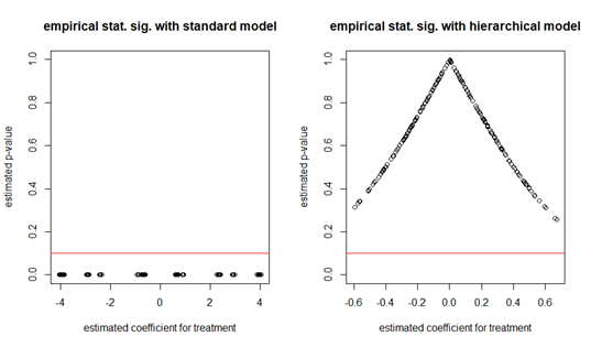
Figure 4-2. Empirical statistical significance with no true effect for standard linear regression (left) and hierarchical regression (right).

Warning

As you may have noticed in figure 10-2, our p-values are vastly off: by definition we should expect to see about 10% of the simulations under the 10% threshold but in reality either 100% of the simulations are under the threshold (with a standard linear regression model) or 0% (with a hierarchical model). This is due to the clustered nature of the data.

Let’s turn to statistical power. With a true treatment effect of 0.5, how often will we see a statistically significant result? We can see on Figure 4-3 that there has been basically no change for the standard linear model—coefficients are still all over the place and appear very significant. On the other hand, coefficients for the hierarchical model have shifted and are now mostly positive, with 89% of them at zero or above; their mean is 0.5, which means they’re unbiased; but only about 2% of them are statistically significant at the 10% s.s. level (i.e. under the horizontal line).

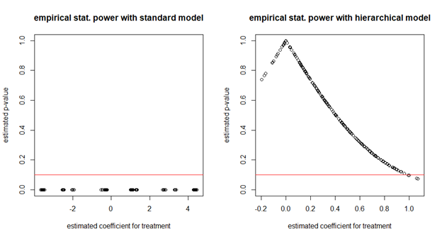
Figure 4-3. Empirical statistical power with a true effect of 0.5 for standard linear regression (left) and hierarchical regression (right).

This means that our power to catch a 0.5 effect at the 10% s.s. level is almost nil. Our power increases quickly with the effect size: running the previous simulation with a 1 effect size gives us an 89% power at the 10% s.s. level.

What should we do? Unfortunately, there is no rule here, it will ultimately be a judgment call—which is precisely the reason why I designed the case study like this. There is nothing wrong or unusual with the situation at hand, but it lands in a grey area and your job is to clearly lay out to the decision-makers what their options are and what are the corresponding trade-offs. The way I see it, there are several options:

• Implement the intervention across the board without running an experiment. I don’t think that’s a good idea, because it would mean that you learn exactly nothing and you take the risk that the intervention has a strong negative effect.

• Run the experiment as designed and stick with a 10% (or even 5%) s.s. level, with the knowledge that you’ll be quite safe from a false positive but will have a high risk of a false negative (i.e. not seeing a s.s. positive effect when indeed there is one). This is a very conservative and statistically sound approach, which minimizes the potential downside at the cost of limiting the upside. However, if you keep shooting down business initiatives as not statistically significant, you take the risk in the long run of finding yourself out of a client or worse, out of a job!

• Run the experiment as designed and change your decision rule to implementing the treatment if the estimated treatment effect is above a certain economic threshold (e.g. 0.75 or 1, to give yourself some margin of error) regardless of its statistical significance. This is a bolder approach, which would raise eyebrows in many quarters, but it’s also probably the closest you can get to maximizing your expected profit without using a full-fledged Bayesian framework.

Which one you or your business partner picks depends on your risk appetite. The data analysis will remain the same, only the decision rule based on it will change. Once you’ve made your decision, you can get to the random assignment and actually run the experiment.

Analyzing the experiment

Once you have run your experiment, you can collect and analyze the data. We’ll apply our hierarchical model, which hopefully should be familiar to you after your power simulations (Example 10-2).

Example 10-2. Hierarchical analysis of the experimental data

## R (output not shown)
> h_mod <- lmer(data=exp_data, call_CSAT ~ reason + age + group + (1|center_ID))
> summary(h_mod)

## Python
h_mod = sm.mixedlm("call_CSAT ~ reason + age + group", data = exp_data_df,
groups = exp_data_df["center_ID"])
print(h_mod.fit().summary())
           Mixed Linear Model Regression Results
============================================================
Model:              MixedLM Dependent Variable: call_CSAT
No. Observations:   71634   Method:             REML
No. Groups:         30      Scale:              1.6522
Min. group size:    1256    Log-Likelihood:     -119759.2898
Max. group size:    3901    Converged:          Yes
Mean group size:    2387.8
------------------------------------------------------------
                   Coef. Std.Err.   z    P>|z| [0.025 0.975]
------------------------------------------------------------
Intercept          3.370    0.416  8.095 0.000  2.554  4.185
reason[T.property] 0.209    0.010 20.641 0.000  0.189  0.229
group[T.treat]     0.827    0.588  1.405 0.160 -0.326  1.979
age                0.020    0.000 45.785 0.000  0.019  0.020
Group Var          2.594    0.534
============================================================

We can see here that the coefficient for our treatment variable is 0.827, with a p-value of 0.16. Depending on the decision rule you’ve picked, you should either decide that the effect is not statistically significant and therefore the intervention should not be implemented, or decide that the effect appears economically significant and therefore the interventions should be implemented.

Alternatively, you can decide to dig deeper into the data, to determine if the treatment was more effective for certain reps (e.g. the most compliant reps) or for certain customers (e.g. certain demographics). Unfortunately, in the case at hand, increasing the sample size by running the experiment longer wouldn’t help much if at all, due to the hierarchical (aka clustered) nature of our experimental units.

Chapter Conclusion

This concludes our tour of experimental design. In the next two chapters (chapter 11 and 12), we’ll see advanced tools that will allow us to dig deeper in the analysis of experimental data, but the call center experiment we’ve just seen is about as complex as experiments get in real life. Being unable to randomize at the lowest level and having a predetermined amount of time to run an experiment are unpleasant but not infrequent circumstances. Randomizing at the level of an office or a store instead of customers or employees is common, to avoid logistical complications and “leakage” between experimental groups. Leveraging simulations for power analysis and stratification for random assignment becomes pretty much unavoidable if you want to get useful results out of your experiment; hopefully you should now be fully equipped to do so.

Designing and running experiments is in my opinion one of the most fun parts of behavioral science. When everything goes well, you get to measure with clarity the impact of a business initiative or a behavioral science intervention. But getting everything to go well is no small feat in itself. Popular media and business vendors often feed the impression that experimentation can be as simple as “plug and play, check for 5% significance and you’re done!”, but this is misleading, and I’ve tried to address several misconceptions that come out of this.

First of all, statistical significance and power are often misunderstood, which can lead to wasted experiments and suboptimal decisions. As I’ve shown you across 3 different case studies, simulations can provide you with a much more nuanced understanding of what an experiment might say and how to interpret it.

Second, treating experiments as a pure technology and data analysis problem is easier but less fruitful than adopting a behavioral-causal approach. Using causal diagrams allows you to articulate more clearly what would be a success and what makes you believe your treatment would be successful.

Implementing an offline experiment in the field is fraught with difficulties (see Glennerster & Takavarasha (2013) for an in-depth discussion), and unfortunately each experiment is different, therefore I can only give you some generic advice (see tip box).

References

Gelman & Hill, Data Analysis Using Regression and Multilevel/Hierarchical Models, Cambridge University Press, 2006. Provides a deeper analysis of multilevel (i.e. clustered) data, at the cost of a higher threshold for mathematical and statistical knowledge.

Gerber & Green, Field Experiments – Design, Analysis and Interpretation, W. W. Norton & Company, 2012. My go-to book for a deeper perspective on experimental design. It contains a lot of statistical and mathematical equations but these should be understandable by anyone with even a moderate quantitative background.

Glennerster & Takavarasha, Running randomized evaluations – a practical guide, Princeton University Press, 2013. An accessible introduction to experimentation in the context of development economics and aid. Contains extensive discussions of the empirical challenges of running “offline” experiments.

Exercises

Exercise 1 (R).

In chapter 5, we analyzed a real-life dataset of hotel bookings. Because I was running a standard linear regression, I had to aggregate most countries in the Country variable into “Other” to keep things manageable. Using the glmer function from the lme4 package in R, can you run a hierarchical logistic regression instead? (warning: the glmer function can be slow and unstable, so run a regression on NRDeposit and Country only, at least to start with).