
Modular Reduction
6.1 Basics of Modular Reduction
Modular reduction arises quite often within public key cryptography algorithms and various number theoretic algorithms, such as factoring. Modular reduction algorithms are the third class of algorithms of the “multipliers” set. A number a is said to be reduced modulo another number b by finding the remainder of the division a/b. Full integer division with remainder is covered in Section 8.1.
Modular reduction is equivalent to solving for r in the following equation: a= bq+ r where q= ![]() . The result r is said to be “congruent to a modulo b,” which is also written as r≡a(mod b). In other vernacular, r is known as the “modular residue,” which leads to “quadratic residue”1 and other forms of residues.
. The result r is said to be “congruent to a modulo b,” which is also written as r≡a(mod b). In other vernacular, r is known as the “modular residue,” which leads to “quadratic residue”1 and other forms of residues.
Modular reductions are normally used to create finite groups, rings, or fields. The most common usage for performance driven modular reductions is in modular exponentiation algorithms; that is, to compute d= ab (mod c) as fast as possible. This operation is used in the RSA and Diffie-Hellman public key algorithms, for example. Modular multiplication and squaring also appears as a fundamental operation in elliptic curve cryptographic algorithms. As will be discussed in the subsequent chapter, there exist fast algorithms for computing modular exponentiations without having to perform (in this example) b−1 multiplications. These algorithms will produce partial results in the range 0≤ x< c2, which can be taken advantage of to create several efficient algorithms. They have also been used to create redundancy check algorithms known as CRCs, error correction codes such as Reed-Solomon, and solve a variety of number theoretic problems.
6.2 The Barrett Reduction
The Barrett reduction algorithm [6] was inspired by fast division algorithms that multiply by the reciprocal to emulate division. Barrett’s observation was that the residue c of a modulo b is equal to
Since algorithms such as modular exponentiation would be using the same modulus extensively, typical DSP2 intuition would indicate the next step would be to replace a/b by a multiplication by the reciprocal. However, DSP intuition on its own will not work, as these numbers are considerably larger than the precision of common DSP floating point data types. It would take another common optimization to optimize the algorithm.
6.2.1 Fixed Point Arithmetic
The trick used to optimize equation 6.1 is based on a technique of emulating floating point data types with fixed precision integers. Fixed point arithmetic would become very popular, as it greatly optimized the “3D-shooter” genre of games in the mid 1990s when floating point units were fairly slow, if not unavailable. The idea behind fixed point arithmetic is to take a normal k-bit integer data type and break it into p-bit integer and a q-bit fraction part (where p+ q= k).
In this system, a k-bit integer n would actually represent n/ 2q. For example, with q= 4 the integer n=37 would actually represent the value 2.3125. To multiply two fixed point numbers, the integers are multiplied using traditional arithmetic and subsequently normalized by moving the implied decimal point back to where it should be. For example, with q= 4, to multiply the integers 9 and 5 they must be converted to fixed point first by multiplying by 2q. Let a= 9(2q) represent the fixed point representation of 9, and b= 5(2q) represent the fixed point representation of 5. The product ab is equal to 45(22q), which when normalized by dividing by 2q produces 45(2q).
This technique became popular since a normal integer multiplication and logical shift right are the only required operations to perform a multiplication of two fixed point numbers. Using fixed point arithmetic, division can be easily approximated by multiplying by the reciprocal. If 2qis equivalent to one, then, 2q/bis equivalent to the fixed point approximation of 1/b using real arithmetic. Using this fact, dividing an integer a by another integer b can be achieved with the following expression.
The precision of the division is proportional to the value of q. If the divisor b is used frequently, as is the case with modular exponentiation, pre-computing 2q/bwill allow a division to be performed with a multiplication and a right shift. Both operations are considerably faster than division on most processors.
Consider dividing 19 by 5. The correct result is ![]() 19/5
19/5![]() =3. With q=3, the reciprocal is
=3. With q=3, the reciprocal is ![]() 2q/5
2q/5![]() = 1, which leads to a product of 19, which when divided by 2q produces 2. However, with q= 4 the reciprocal is
= 1, which leads to a product of 19, which when divided by 2q produces 2. However, with q= 4 the reciprocal is ![]() 2q/5
2q/5![]() =3 and the result of the emulated division is
=3 and the result of the emulated division is ![]() 3 · 19/2q
3 · 19/2q![]() =3, which is correct. The value of 2q must be close to or ideally larger than the dividend. In effect, if a is the dividend, then q should allow 0≤
=3, which is correct. The value of 2q must be close to or ideally larger than the dividend. In effect, if a is the dividend, then q should allow 0≤![]() a/2q
a/2q![]() ≤1 for this approach to work correctly. Plugging this form of division into the original equation, the following modular residue equation arises.
≤1 for this approach to work correctly. Plugging this form of division into the original equation, the following modular residue equation arises.
Using the notation from [6], the value of ![]() 2q/b
2q/b![]() will be represented by the μ symbol. Using the μ variable also helps reinforce the idea that it is meant to be computed once and re-used.
will be represented by the μ symbol. Using the μ variable also helps reinforce the idea that it is meant to be computed once and re-used.
Provided that 2q ≥ a, this algorithm will produce a quotient that is either exactly correct or off by a value of one. In the context of Barrett reduction the value of a is bound by 0 ≤ a ≤ (b−1)2, meaning that 2q ≥ b2 is sufficient to ensure the reciprocal will have enough precision.
Let n represent the number of digits in b. This algorithm requires approximately 2n2 single precision multiplications to produce the quotient, and another n2 single precision multiplications to find the residue. In total, 3n2 single precision multiplications are required to reduce the number.
For example, if b= 1179677 and q= 41 (2q> b2), the reciprocal μ is equal to ![]() 2q/b
2q/b![]() = 1864089. Consider reducing a= 180388626447 modulo b using the preceding reduction equation. The quotient using the new formula is
= 1864089. Consider reducing a= 180388626447 modulo b using the preceding reduction equation. The quotient using the new formula is ![]() (a.μ)/2q
(a.μ)/2q![]() = 152913. By subtracting 152913b from a, the correct residue a= 677346 (mod b) is found.
= 152913. By subtracting 152913b from a, the correct residue a= 677346 (mod b) is found.
6.2.2 Choosing a Radix Point
Using the fixed point representation, a modular reduction can be performed with 3n2 single precision multiplications3. If that were the best that could be achieved. a full division4 might as well be used in its place. The key to optimizing the reduction is to reduce the precision of the initial multiplication that finds the quotient.
Let a represent the number of which the residue is sought. Let b represent the modulus used to find the residue. Let m represent the number of digits in b. For the purposes of this discussion we will assume that the number of digits in a is 2m, which is generally true if two m-digit numbers have been multiplied. Dividing a by b is the same as dividing a 2m digit integer by an m digit integer. Digits below the m−1′th digit of a will contribute at most a value of 1 to the quotient, because βk<bfor any 0≤ k ≤ m−1. Another way to express this is by re-writing a as two parts. If a′≡ a(mod bm)and a″=a−a′, then![]() which is equivalent to
which is equivalent to![]() Since a′is bound to be less than b, the quotient is bound by 0≤
Since a′is bound to be less than b, the quotient is bound by 0≤![]() <1.
<1.
Since the digits of a′do not contribute much to the quotient the observation is that they might as well be zero. However, if the digits “might as well be zero,” they might as well not be there in the first place. Let q0 = ![]() a/βm−1
a/βm−1![]() represent the input with the irrelevant digits trimmed. Now the modular reduction is trimmed to the almost equivalent equation
represent the input with the irrelevant digits trimmed. Now the modular reduction is trimmed to the almost equivalent equation
Note that the original divisor 2q has been replaced with βm+1 where in this case q is a multiple of lg(β). Also note that the exponent on the divisor when added to the amount q0 was shifted by equals 2m. If the optimization had not been performed the divisor would have the exponent 2m, so in the end the exponents do “add up.” Using equation 6.5 the quotient![]() (q0 · μ)/βm+1
(q0 · μ)/βm+1![]() can be off from the true quotient by at most two. The original fixed point quotient can be off by as much as one (provided the radix point is chosen suitably), and now that the lower irrelevant digits have been trimmed the quotient can be off by an additional value of one for a total of at most two. This implies that 0≤ a− b ·
can be off from the true quotient by at most two. The original fixed point quotient can be off by as much as one (provided the radix point is chosen suitably), and now that the lower irrelevant digits have been trimmed the quotient can be off by an additional value of one for a total of at most two. This implies that 0≤ a− b · ![]() (q0 · μ)/βm+1
(q0 · μ)/βm+1![]() <3b. By first subtracting b times the quotient and then conditionally subtracting b once or twice the residue is found.
<3b. By first subtracting b times the quotient and then conditionally subtracting b once or twice the residue is found.
The quotient is now found using (m + 1)(m) = m2 + m single precision multiplications and the residue with an additional m2 single precision multiplications, ignoring the subtractions required. In total, 2m2 + m single precision multiplications are required to find the residue. This is considerably faster than the original attempt.
For example, let β= 10 represent the radix of the digits. Let b= 9999 represent the modulus, which implies m= 4. Let a= 99929878 represent the value of which the residue is desired; in this case, q= 8 since 107<99992, meaning that μ=![]() βq/b
βq/b![]() = 10001. With the new observation the multiplicand for the quotient is equal to q0 =
= 10001. With the new observation the multiplicand for the quotient is equal to q0 =![]() a/βm−1
a/βm−1![]() = 99929. The quotient is then
= 99929. The quotient is then![]() (q0 · μ)/βm+1
(q0 · μ)/βm+1![]() = 9993. Subtract 9993b from a and the correct residue a= 9871 (mod b) is found.
= 9993. Subtract 9993b from a and the correct residue a= 9871 (mod b) is found.
6.2.3 Trimming the Quotient
So far, the reduction algorithm has been optimized from 3m2 single precision multiplications down to 2m2+ m single precision multiplications. As it stands now, the algorithm is already fairly fast compared to a full integer division algorithm. However, there is still room for optimization.
After the first multiplication inside the quotient (q0 · μ) the value is shifted right by m + 1 places, effectively nullifying the lower half of the product. It would be nice to be able to remove those digits from the product to effectively cut down the number of single precision multiplications. If the number of digits in the modulus m is far less than β, a full product is not required for the algorithm to work properly. In fact, the lower m−2 digits will not affect the upper half of the product at all and do not need to be computed.
The value of μ is an m-digit number and q0 is an m + 1 digit number. Using a full multiplier (m + 1)(m) = m2 + m single precision multiplications would be required. Using a multiplier that will only produce digits at and above the m−1′th digit reduces the number of single precision multiplications to m2+m/2 single precision multiplications.
6.2.4 Trimming the Residue
After the quotient has been calculated it is used to reduce the input. As previously noted, the algorithm is not exact and can be off by a small multiple of the modulus; that is, 0≤ a− b · ![]() (q0 · μ)/βm+1
(q0 · μ)/βm+1![]() <3b. If b is m digits, the result of reduction equation is a value of at most m + 1 digits (provided 3<β) implying that the upper m−1 digits are implicitly zero.
<3b. If b is m digits, the result of reduction equation is a value of at most m + 1 digits (provided 3<β) implying that the upper m−1 digits are implicitly zero.
The next optimization arises from this very fact. Instead of computing b · ![]() (q0 · μ)/βm+1
(q0 · μ)/βm+1![]() using a full O(m2) multiplication algorithm, only the lower m + 1 digits of the product have to be computed. Similarly, the value of a can be reduced modulo βm+1 before the multiple of b is subtracted, which simplifies the subtraction as well. A multiplication that produces only the lower m + 1 digits requires
using a full O(m2) multiplication algorithm, only the lower m + 1 digits of the product have to be computed. Similarly, the value of a can be reduced modulo βm+1 before the multiple of b is subtracted, which simplifies the subtraction as well. A multiplication that produces only the lower m + 1 digits requires![]() single precision multiplications.
single precision multiplications.
With both optimizations in place the algorithm is the algorithm Barrett proposed. It requires m2 + 2m−1 single precision multiplications, which are considerably faster than the straightforward 3m2 method.
6.2.5 The Barrett Algorithm
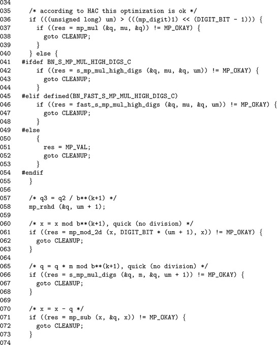
Algorithm mp_reduce. This algorithm will reduce the input a modulo 6 in place using the Barrett algorithm. It is loosely based on algorithm 14.42 of HAC [2, pp. 602], which is based on the paper from Paul Barrett [6]. The algorithm has several restrictions and assumptions that must be adhered to for the algorithm to work (Figure 6.1).
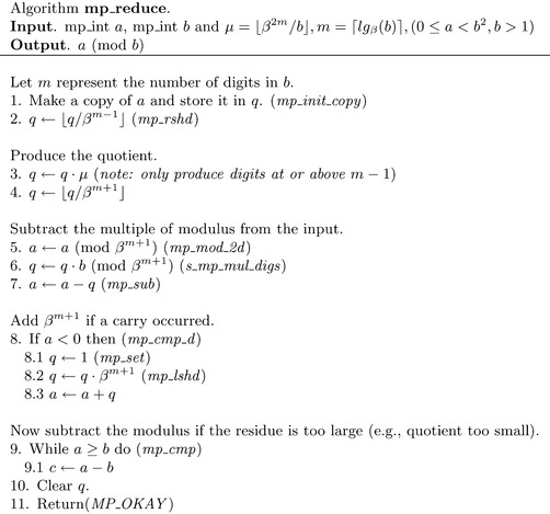
First, the modulus b is assumed positive and greater than one. If the modulus were less than or equal to one, subtracting a multiple of it would either accomplish nothing or actually enlarge the input. The input a must be in the range 0 ≤ a< b2for the quotient to have enough precision. If a is the product of two numbers that were already reduced modulo b, this will not be a problem. Technically, the algorithm will still work if a ≥ b2 but it will take much longer to finish. The value of μ is passed as an argument to this algorithm and is assumed calculated and stored before the algorithm is used.
Recall that the multiplication for the quotient in step 3 must only produce digits at or above the m−1′th position. An algorithm called s_mp_mul_high_digs that has not been presented is used to accomplish this task. The algorithm is based on s_mp_mul_digs, except that instead of stopping at a given level of precision it starts at a given level of precision. This optimal algorithm can only be used if the number of digits in b is much smaller than β.
While it is known that a ≥ b · ![]() (q0 · μ)/βm+1
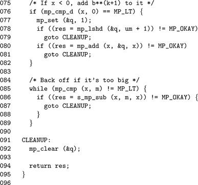
(q0 · μ)/βm+1![]() , only the lower m + 1 digits are being used to compute the residue, so an implied “borrow” from the higher digits might leave a negative result. After the multiple of the modulus has been subtracted from a, the residue must be fixed up in case it is negative. The invariant βm+1 must be added to the residue to make it positive again.
, only the lower m + 1 digits are being used to compute the residue, so an implied “borrow” from the higher digits might leave a negative result. After the multiple of the modulus has been subtracted from a, the residue must be fixed up in case it is negative. The invariant βm+1 must be added to the residue to make it positive again.
The while loop in step 9 will subtract b until the residue is less than b. If the algorithm is performed correctly, this step is performed at most twice, and on average once. However, if a ≥ b2, it will iterate substantially more times than it should.
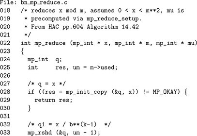
The first multiplication that determines the quotient can be performed by only producing the digits from m−1 and up. This essentially halves the number of single precision multiplications required. However, the optimization is only safe if β is much larger than the number of digits in the modulus. In the source code, this is evaluated on lines 36 to 44 where algorithm s_mp_mul_high_digs is used when it is safe to do so.
6.2.6 The Barrett Setup Algorithm
To use algorithm mp_reduce, the value of μ must be calculated in advance. Ideally, this value should be computed once and stored for future use so the Barrett algorithm can be used without delay.
Algorithm mp_reduce_setup. This algorithm computes the reciprocal μ required for Barrett reduction. First, β2m is calculated as 22.lg(β).m, which is equivalent and much faster. The final value is computed by taking the integer quotient of ![]() μ/b
μ/b![]() (Figure 6.2).
(Figure 6.2).
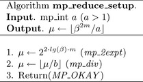
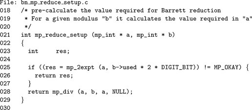
This simple routine calculates the reciprocal μrequired by Barrett reduction. Note the extended usage of algorithm mp_div where the variable that would receive the remainder is passed as NULL. As will be discussed in 8.1, the division routine allows both the quotient and the remainder to be passed as NULL, meaning to ignore the value.
6.3 The Montgomery Reduction
Montgomery reduction5 [6] is by far the most interesting form of reduction in common use. It computes a modular residue that is not actually equal to the residue of the input, yet instead equal to a residue times a constant. However, as perplexing as this may sound, the algorithm is relatively simple and very efficient.
Throughout this entire section the variable n will represent the modulus used to form the residue. As will be discussed shortly, the value of n must be odd. The variable x will represent the quantity of which the residue is sought. Similar to the Barrett algorithm, the input is restricted to 0 ≤ x< n2. To begin the description, some simple number theory facts must be established.
Fact 1. Adding n to x does not change the residue, since in effect it adds one to the quotient ![]() x/n
x/n![]() . Another way to explain this is that n is (or multiples of n are) congruent to zero modulo n. Adding zero will not change the value of the residue.
. Another way to explain this is that n is (or multiples of n are) congruent to zero modulo n. Adding zero will not change the value of the residue.
Fact 2. If x is even, then performing a division by two in ![]() is congruent to x · 2−1 (mod n). Actually, this is an application of the fact that if x is evenly divisible by any k∈
is congruent to x · 2−1 (mod n). Actually, this is an application of the fact that if x is evenly divisible by any k∈![]() , then division in
, then division in ![]() will be congruent to multiplication by k−1 modulo n.
will be congruent to multiplication by k−1 modulo n.
From these two simple facts the following simple algorithm can be derived.
The algorithm in Figure 6.3 reduces the input one bit at a time using the two congruencies stated previously. Inside the loop n, which is odd, is added to x if x is odd. This forces x to be even, which allows the division by two in ![]() to be congruent to a modular division by two. Since x is assumed initially much larger than n, the addition of n will contribute an insignificant magnitude to x. Let r represent the result of the Montgomery algorithm. If k>lg(n) and 0 ≤ x<n2, then the result is limited to 0≤ r<
to be congruent to a modular division by two. Since x is assumed initially much larger than n, the addition of n will contribute an insignificant magnitude to x. Let r represent the result of the Montgomery algorithm. If k>lg(n) and 0 ≤ x<n2, then the result is limited to 0≤ r<![]() x/2k
x/2k![]() +n. At most, a single subtraction is required to get the residue desired.
+n. At most, a single subtraction is required to get the residue desired.
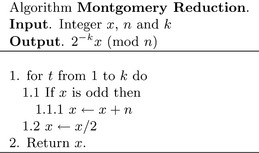
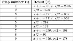
Consider the example in Figure 6.4, which reduces x= 5555 modulo n = 257 when k = 9 (note βk= 512, which is larger than n). The result of the algorithm r= 178 is congruent to the value of 2−9 · 5555 (mod 257). When r is multiplied by 29 modulo 257, the correct residue r = 158 is produced.
Let k= ![]() lg(n)
lg(n)![]() + 1 represent the number of bits in n. The current algorithm requires 2k2 single precision shifts and k2 single precision additions. At this rate, the algorithm is most certainly slower than Barrett reduction and not terribly useful. Fortunately, there exists an alternative representation of the algorithm.
+ 1 represent the number of bits in n. The current algorithm requires 2k2 single precision shifts and k2 single precision additions. At this rate, the algorithm is most certainly slower than Barrett reduction and not terribly useful. Fortunately, there exists an alternative representation of the algorithm.
This algorithm is equivalent since 2tn is a multiple of n and the lower k bits of x are zero by step 2. The number of single precision shifts has now been reduced from 2k2 to k2 + k, which is only a small improvement (Figure 6.5).
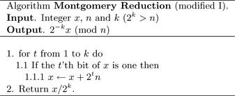
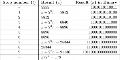
Figure 6.6 demonstrates the modified algorithm reducing x = 5555 modulo n= 257 with k= 9. With this algorithm, a single shift right at the end is the only right shift required to reduce the input instead of k right shifts inside the loop. Note that for the iterations t= 2, 5, 6, and 8 where the result x is not changed. In those iterations the t′th bit of x is zero and the appropriate multiple of n does not need to be added to force the t′th bit of the result to zero.
6.3.1 Digit Based Montgomery Reduction
Instead of computing the reduction on a bit-by-bit basis it is much faster to compute it on digit-by-digit basis. Consider the previous algorithm re-written to compute the Montgomery reduction in this new fashion (Figure 6.7).
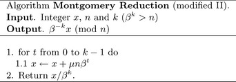
The value μnβt is a multiple of the modulus n, meaning that it will not change the residue. If the first digit of the value μnβtequals the negative (modulo β) of the t′th digit of x, then the addition will result in a zero digit. This problem breaks down to solving the following congruency.
In each iteration of the loop in step 1 a new value of μ must be calculated. The value of−1/n0 (mod β) is used extensively in this algorithm and should be precomputed. Let ρ represent the negative of the modular inverse of n0 modulo β.
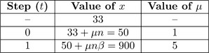
For example, let β= 10 represent the radix. Let n= 17 represent the modulus, which implies k= 2 and ρ≡7. Let x= 33 represent the value to reduce.
The result in Figure 6.8 of 900 is then divided by βkto produce the result 9. The first observation is that 9![]() x (mod n), which implies the result is not the modular residue of x modulo n. However, recall that the residue is actually multiplied by β−kin the algorithm. To get the true residue the value must be multiplied by βk. In this case, βk≡15 (mod n) and the correct residue is 9 · 15 = 16 (mod n).
x (mod n), which implies the result is not the modular residue of x modulo n. However, recall that the residue is actually multiplied by β−kin the algorithm. To get the true residue the value must be multiplied by βk. In this case, βk≡15 (mod n) and the correct residue is 9 · 15 = 16 (mod n).
6.3.2 Baseline Montgomery Reduction
The baseline Montgomery reduction algorithm will produce the residue for any size input. It is designed to be a catch-all algorithm for Montgomery reductions.
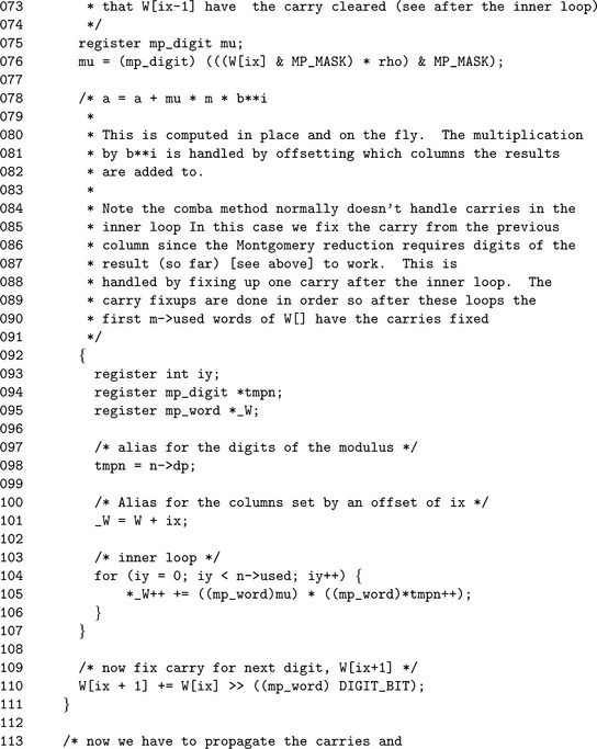
Algorithm mp_montgomery_reduce. This algorithm reduces the input x modulo n in place using the Montgomery reduction algorithm. The algorithm is loosely based on algorithm 14.32 of [2, pp.601], except it merges the multiplication of μnβt with the addition in the inner loop. The restrictions on this algorithm are fairly easy to adapt to. First, 0 ≤ x< n2 bounds the input to numbers in the same range as for the Barrett algorithm. Additionally, if n>1 and n is odd there will exist a modular inverse ρ. ρ must be calculated in advance of this algorithm. Finally, the variable k is fixed and a pseudonym for n.used(Figure 6.9).
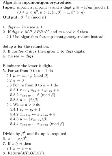
Step 2 decides whether a faster Montgomery algorithm can be used. It is based on the Comba technique, meaning that there are limits on the size of the input. This algorithm is discussed in 7.9.
Step 5 is the main reduction loop of the algorithm. The value of μ is calculated once per iteration in the outer loop. The inner loop calculates x + μnβixby multiplying μn and adding the result to x shifted by ix digits. Both the addition and multiplication are performed in the same loop to save time and memory. Step 5.4 will handle any additional carries that escape the inner loop.
On quick inspection, this algorithm requires n single precision multiplications for the outer loop and n2 single precision multiplications in the inner loop for a total n2 + n single precision multiplications, which compares favorably to Barrett at n2 + 2n−1 single precision multiplications.
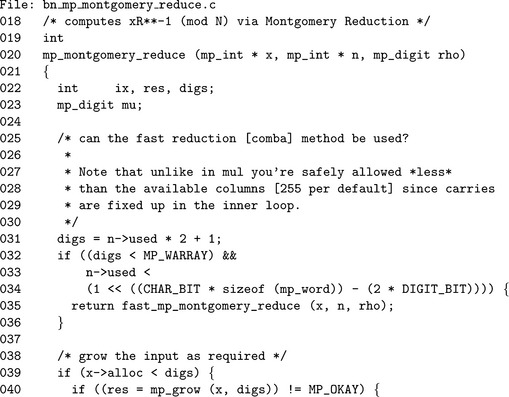
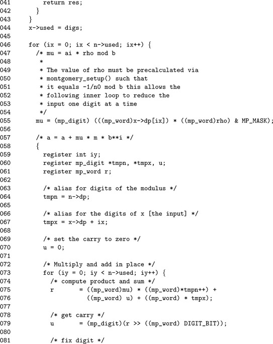
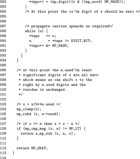
This is the baseline implementation of the Montgomery reduction algorithm. Lines 31 to 36 determine if the Comba–based routine can be used instead. Line 47 computes the value of μ for that particular iteration of the outer loop.
The multiplication μnβixis performed in one step in the inner loop. The alias tmpx refers to the ix′th digit of x, and the alias tmpn refers to the modulus n.
6.3.3 Faster “Comba” Montgomery Reduction
The Montgomery reduction requires fewer single precision multiplications than a Barrett reduction; however, it is much slower due to the serial nature of the inner loop. The Barrett reduction algorithm requires two slightly modified multipliers, which can be implemented with the Comba technique. The Montgomery reduction algorithm cannot directly use the Comba technique to any significant advantage since the inner loop calculates a k×1 product k times.
The biggest obstacle is that at the ix′th iteration of the outer loop, the value of xix is required to calculate μ. This means the carries from 0 to ix−1 must have been propagated upwards to form a valid ix′th digit. The solution as it turns out is very simple. Perform a Comba–like multiplier, and inside the outer loop just after the inner loop, fix up the ix + 1′th digit by forwarding the carry.
With this change in place, the Montgomery reduction algorithm can be performed with a Comba–style multiplication loop, which substantially increases the speed of the algorithm.
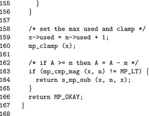
Algorithm fast_mp_montgomery_reduce. This algorithm will compute the Montgomery reduction of x modulo n using the Comba technique. It is on most computer platforms significantly faster than algorithm mp_montgomery_reduce and algorithm mp_reduce (Barrett reduction). The algorithm has the same restrictions on the input as the baseline reduction algorithm. An additional two restrictions are imposed on this algorithm. The number of digits k in the modulus n must not violate MP_W ARRAY > 2k+1 and n<δ. When β= 228, this algorithm can be used to reduce modulo a modulus of at most 3, 556 bits in length (Figure 6.10).
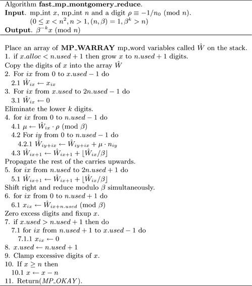
As in the other Comba reduction algorithms there is a Ŵ array that stores the columns of the product. It is initially filled with the contents of x with the excess digits zeroed. The reduction loop is very similar the to the baseline loop at heart. The multiplication in step 4.1 can be single precision only, since ab(mod β) = (a mod β) (b mod β). Some multipliers such as those on the ARM processors take a variable length time to complete depending on the number of bytes of result it must produce. By performing a single precision multiplication instead, half the amount of time is spent.
Also note that digit Ŵix must have the carry from the ix−1′th digit propagated upwards for this to work. That is what step 4.3 will do. In effect, over the n.used iterations of the outer loop the n.used′th lower columns all have their carries propagated forwards. Note how the upper bits of those same words are not reduced modulo β. This is because those values will be discarded shortly and there is no point.
Step 5 will propagate the remainder of the carries upwards. In step 6, the columns are reduced modulo β and shifted simultaneously as they are stored in the destination x.
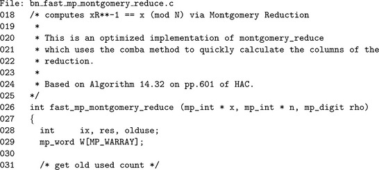
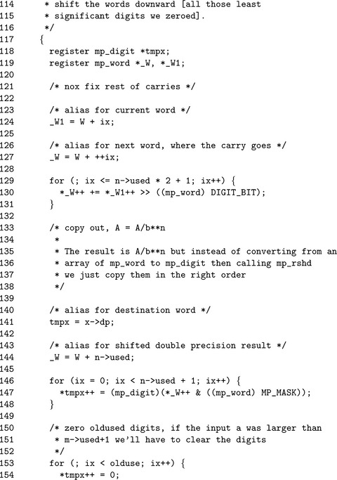
The Ŵ array is first filled with digits of x on Line 55, then the rest of the digits are zeroed on Line 60. Both loops share the same alias variables to make the code easier to read.
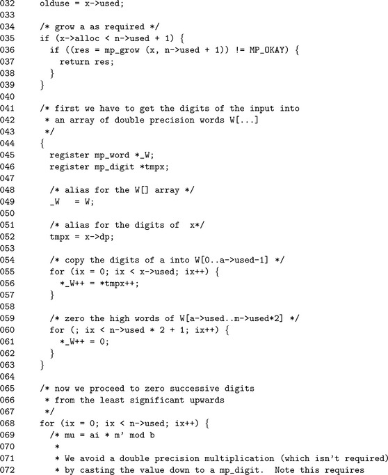
The value of μ is calculated in an interesting fashion. First, the value Ŵixis reduced modulo β and cast to a mp_digit. This forces the compiler to use a single precision multiplication and prevents any concerns about loss of precision. Line 110 fixes the carry for the next iteration of the loop by propagating the carry from Ŵixto Ŵix+1.
The for loop on Line 129 propagates the rest of the carries upwards through the columns. The for loop on Line 146 reduces the columns modulo β and shifts them k places at the same time. The alias _Ŵactually refers to the array Ŵ starting at the n.used′th digit, that is _Ŵt=Ŵn.used+t.
6.3.4 Montgomery Setup
To calculate the variable ρ, a relatively simple algorithm will be required.
Algorithm mp_montgomery_setup. This algorithm will calculate the value of ρ required within the Montgomery reduction algorithms. It uses a very interesting trick to calculate 1/n0 when βis a power of two (Figure 6.11).
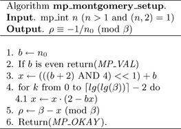
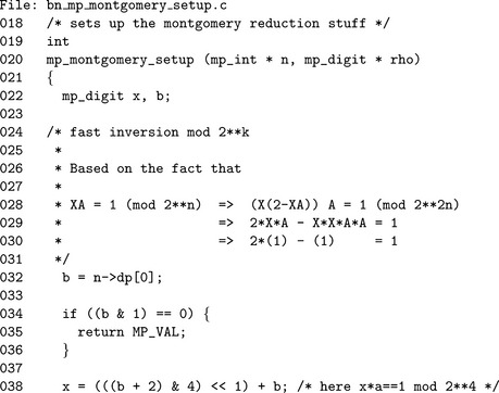
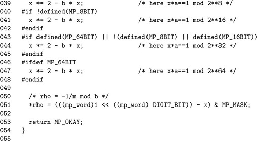
This source code computes the value of ρ required to perform Montgomery reduction. It has been modified to avoid performing excess multiplications when β is not the default 28 bits.
6.4 The Diminished Radix Algorithm
The Diminished Radix method of modular reduction [6] is a fairly clever technique that can be more efficient than either the Barrett or Montgomery methods for certain forms of moduli. The technique is based on the following simple congruence.
This observation was used in the MMB [6] block cipher to create a diffusion primitive. It used the fact that if n= 231 and k= 1, an x86 multiplier could produce the 62-bit product and use the “shrd” instruction to perform a double-precision right shift. The proof of equation 6.6 is very simple. First, write x in the product form.
Now reduce both sides modulo (n− k).
The variable n reduces modulo n− k to k. By putting q = ![]() x/n
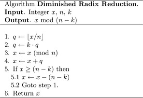
x/n![]() and r= x mod n into the equation the original congruence is reproduced, thus concluding the proof. The following algorithm is based on this observation.
and r= x mod n into the equation the original congruence is reproduced, thus concluding the proof. The following algorithm is based on this observation.
This algorithm will reduce x modulo n− k and return the residue. If 0 ≤ x<(n− k)2, then the algorithm will loop almost always once or twice and occasionally three times. For simplicity’s sake, the value of x is bounded by the following simple polynomial.
The true bound is 0 ≤ x<(n− k−1)2, but this has quite a few more terms. The value of q after step 1 is bounded by the following equation.
Since k2 is going to be considerably smaller than n, that term will always be zero. The value of x after step 3 is bounded trivially as 0 ≤ x< n. By step 4, the sum x + q is bounded by
With a second pass, q will be loosely bounded by 0 ≤ q< k2 after step 2, while x will still be loosely bounded by 0 ≤ x< n after step 3. After the second pass it is highly unlikely that the sum in step 4 will exceed n− k. In practice, fewer than three passes of the algorithm are required to reduce virtually every input in the range 0 ≤ x<(n− k−1)2.
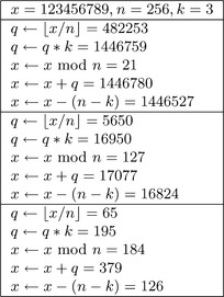
Figure 6.13 demonstrates the reduction of x= 123456789 modulo n− k= 253 when n= 256 and k= 3. Note that even while x is considerably larger than (n− k−1)2 = 63504, the algorithm still converges on the modular residue exceedingly fast. In this case, only three passes were required to find the residue x ≡126.
6.4.1 Choice of Moduli
On the surface, this algorithm looks very expensive. It requires a couple of subtractions followed by multiplication and other modular reductions. The usefulness of this algorithm becomes exceedingly clear when an appropriate modulus is chosen.
Division in general is a very expensive operation to perform. The one exception is when the division is by a power of the radix of representation used. Division by 10, for example, is simple for pencil and paper mathematics since it amounts to shifting the decimal place to the right. Similarly, division by 2 (or powers of 2) is very simple for binary computers to perform. It would therefore seem logical to choose n of the form 2p, which would imply that ![]() x/n
x/n![]() is a simple shift of x right p bits.
is a simple shift of x right p bits.
However, there is one operation related to division of power of twos that is even faster. If n= βp, then the division may be performed by moving whole digits to the right p places. In practice, division by βpis much faster than division by 2pfor any p. Also, with the choice of n= βpreducing x modulo n merely requires zeroing the digits above the p−1′th digit of x.
Throughout the next section the term restricted modulus will refer to a modulus of the form βp−k, whereas the term unrestricted modulus will refer to a modulus of the form 2p− k. The word restricted in this case refers to the fact that it is based on the 2p logic, except p must be a multiple of lg(β).
6.4.2 Choice of k
Now that division and reduction (steps 1 and 3 of Figure 6.12)have been optimized to simple digit operations, the multiplication by k in step 2 is the most expensive operation. Fortunately, the choice of kis not terribly limited. For all intents and purposes it might as well be a single digit. The smaller the value of k, the faster the algorithm will be.
6.4.3 Restricted Diminished Radix Reduction
The Restricted Diminished Radix algorithm can quickly reduce an input modulo a modulus of the form n= βp− k. This algorithm can reduce an input x within the range 0 ≤ x< n2 using only a couple of passes of the algorithm demonstrated in Figure 6.12. The implementation of this algorithm has been optimized to avoid additional overhead associated with a division by βp, the multiplication by k or the addition of x and q. The resulting algorithm is very efficient and can lead to substantial improvements over Barrett and Montgomery reduction when modular exponentiations are performed.
Algorithm mp_dr_reduce. This algorithm will perform the Diminished Radix reduction of x modulo n. It has similar restrictions to that of the Barrett reduction with the addition that n must be of the form n= βm− k where 0< k<β (Figure 6.14).
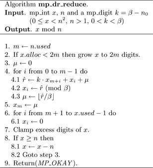
This algorithm essentially implements the pseudo-code in Figure 6.12, except with a slight optimization. The division by βm, multiplication by k, and addition of x mod βm are all performed simultaneously inside the loop in step 4. The division by βm is emulated by accessing the term at the m + i′th position, which is subsequently multiplied by k and added to the term at the i′th position. After the loop the m′th digit is set to the carry and the upper digits are zeroed. Steps 5 and 6 emulate the reduction modulo βm that should have happened to x before the addition of the multiple of the upper half.
In step 8, if x is still larger than n, another pass of the algorithm is required. First, n is subtracted from x and then the algorithm resumes at step 3.
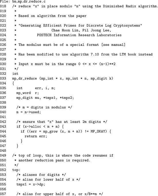
The first step is to grow x as required to 2m digits, since the reduction is performed in place on x. The label on Line 52 is where the algorithm will resume if further reduction passes are required. In theory, it could be placed at the top of the function. However, the size of the modulus and question of whether x is large enough are invariant after the first pass, meaning that it would be a waste of time.
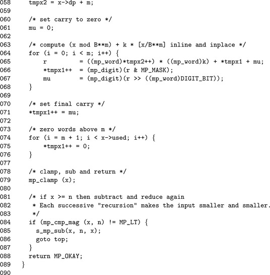
The aliases tmpx 1 and tmpx 2 refer to the digits of x, where the latter is offset by m digits. By reading digits from x offset by m digits, a division by βm can be simulated virtually for free. The loop on Line 64 performs the bulk of the work (corresponds to step 4 of algorithm 7.11) in this algorithm.
By Line 67 the pointer tmpx 1 points to the m′th digit of x, which is where the final carry will be placed. Similarly, by Line 74 the same pointer will point to the m + 1′th digit where the zeroes will be placed.
Since the algorithm is only valid if both x and n are greater than zero, an unsigned comparison suffices to determine if another pass is required. With the same logic at Line 81 the value of x is known to be greater than or equal to n, meaning that an unsigned subtraction can be used as well. Since the destination of the subtraction is the larger of the inputs, the call to algorithm s_mp_sub cannot fail and the return code does not need to be checked.
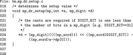
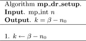
Setup
To set up the Restricted Diminished Radix algorithm the value k= β− n0 is required. This algorithm is not complicated but is provided for completeness (Figure 6.15).
Modulus Detection
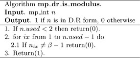
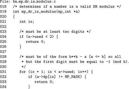
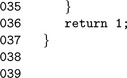
Another useful algorithm gives the ability to detect a Restricted Diminished Radix modulus. An integer is said to be of Restricted Diminished Radix form if all the digits are equal to β− 1 except the trailing digit, which may be any value.
Algorithm mp_dr_is_modulus. This algorithm determines if a value is in Diminished Radix form. step 1 rejects obvious cases where fewer than two digits are in the mp_int. step 2 tests all but the first digit to see if they are equal to β−1. If the algorithm manages to get to step 3, then n must be of Diminished Radix form (Figure 6.16).
6.4.4 Unrestricted Diminished Radix Reduction
The unrestricted Diminished Radix algorithm allows modular reductions to be performed when the modulus is of the form 2p−k. This algorithm is a straightforward adaptation of algorithm 6.12.
In general, the restricted Diminished Radix reduction algorithm is much faster since it has considerably lower overhead. However, this new algorithm is much faster than either Montgomery or Barrett reduction when the moduli are of the appropriate form.
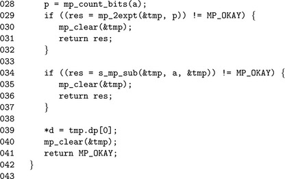
Algorithm mp_reduce_2k. This algorithm quickly reduces an input a modulo an unrestricted Diminished Radix modulus n. Division by 2pis emulated with a right shift, which makes the algorithm fairly inexpensive to use (Figure 6.17).
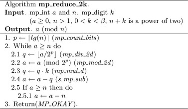
![]()
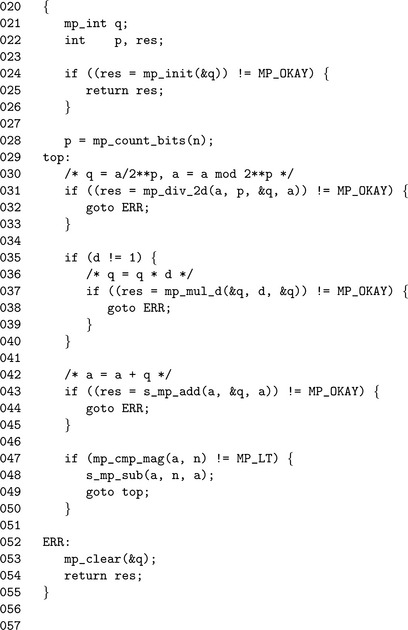
The algorithm mp_count_bits calculates the number of bits in an mp_int, which is used to find the initial value of p. The call to mp_div_2d on Line 31 calculates both the quotient q and the remainder a required. By doing both in a single function call, the code size is kept fairly small. The multiplication by k is only performed if k>1. This allows reductions modulo 2p −1 to be performed without any multiplications.
The unsigned s_mp_add, mp_cmp_mag, and s_mp_sub are used in place of their full sign counterparts since the inputs are only valid if they are positive. By using the unsigned versions, the overhead is kept to a minimum.
Unrestricted Setup
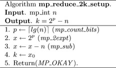
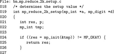
To set up this reduction algorithm, the value of k= 2p−n is required.
Algorithm mp_reduce_2k_setup. This algorithm computes the value of k required for the algorithm mp_reduce_2k. By making a temporary variable x equal to 2p, a subtraction is sufficient to solve for k. Alternatively if n has more than one digit the value of k is simply β− n0 (Figure 6.18).
Unrestricted Detection
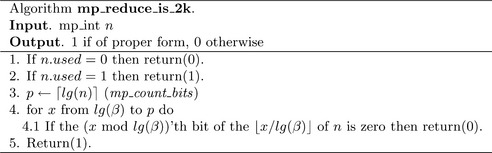
An integer n is a valid unrestricted Diminished Radix modulus if either of the following are true.
• The number has only one digit.
• The number has more than one digit, and every bit from the β′th to the most significant is one.
If either condition is true, there is a power of two 2psuch that 0<2p− n<β. If the input is only one digit, it will always be of the correct form. Otherwise, all of the bits above the first digit must be one. This arises from the fact that there will be value of k that when added to the modulus causes a carry in the first digit that propagates all the way to the most significant bit. The resulting sum will be a power of two.
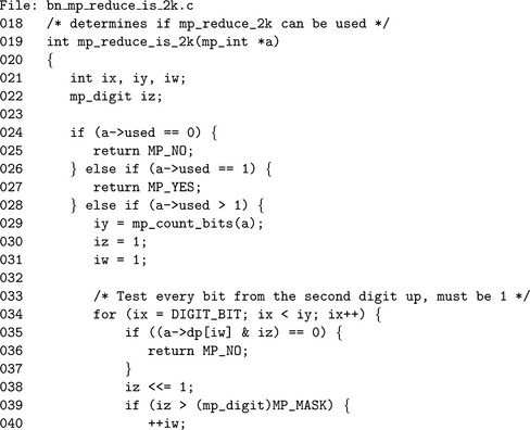
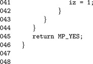
Algorithm mp_reduce_is_2k. This algorithm quickly determines if a modulus is of the form required for algorithm mp_reduce_2k to function properly (Figure 6.19).
6.5 Algorithm Comparison
So far, three very different algorithms for modular reduction have been discussed. Each algorithm has its own strengths and weaknesses that make having such a selection very useful. The following table summarizes the three algorithms along with comparisons of work factors. Since all three algorithms have the restriction that 0 ≤ x< n2 and n> 1, those limitations are not included in the table.
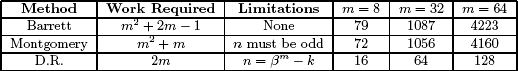
In theory, Montgomery and Barrett reductions would require roughly the same amount of time to complete. However, in practice since Montgomery reduction can be written as a single function with the Comba technique, it is much faster. Barrett reduction suffers from the overhead of calling the half precision multipliers, addition and division by β algorithms.
For almost every cryptographic algorithm, Montgomery reduction is the algorithm of choice. The one set of algorithms where Diminished Radix reduction truly shines is based on the discrete logarithm problem such as Diffie-Hellman and ElGamal. In these algorithms, primes of the form βm− k can be found and shared among users. These primes will allow the Diminished Radix algorithm to be used in modular exponentiation to greatly speed up the operation.
3. Prove that the “trick” in algorithm mp_montgomery_setup actually calculates the correct value of ρ.
2. Devise an algorithm to reduce modulo n + k for small k quickly.
4. Prove that the pseudo-code algorithm “Diminished Radix Reduction” (Figure 6.12)terminates. Also prove the probability that it will terminate within 1 ≤ k ≤ 10 iterations.
1That′s fancy talk for b≡a2 (mod p).
2It is worth noting that Barrett’s paper targeted the DSP56K processor.
4A division requires approximately O(2cn2) single precision multiplications for a small value of c. See 8.1 for further details.
5Thanks to Niels Ferguson for his insightful explanation of the algorithm.