
Number Theoretic Algorithms
This chapter discusses several fundamental number theoretic algorithms such as the greatest common divisor, least common multiple, and Jacobi symbol computation. These algorithms arise as essential components in several key cryptographic algorithms such as the RSA public key algorithm and various sieve-based factoring algorithms.
9.1 Greatest Common Divisor
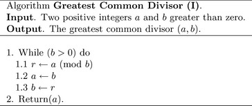
The greatest common divisor of two integers a and b, often denoted as (a, b), is the largest integer k that is a proper divisor of both a and b. That is, k is the largest integer such that 0 = a(mod k) and 0 = b(mod k) occur simultaneously.
The most common approach [1, pp. 337] is to reduce one operand modulo the other operand. That is, if a and b are divisible by some integer k and if qa+ r = b, then r is also divisible by k. The reduction pattern follows 〈 a, b〉→〈 b, a mod b〉.
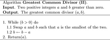
This algorithm will quickly converge on the greatest common divisor since the residue r tends to diminish rapidly (Figure 9.1). However, divisions are relatively expensive operations to perform and should ideally be avoided. There is another approach based on a similar relationship of greatest common divisors. The faster approach is based on the observation that if k divides both a and b, it will also divide a−b. In particular, we would like a−b to decrease in magnitude, which implies that b ≥ a.
Theorem Algorithm 9.2 will return the greatest common divisor of a and b.
Proof The algorithm in Figure 9.2 will eventually terminate; since b≥ a the subtraction in step 1.2 will be a value less than b. In other words, in every iteration that tuple 〈 a, b〉, decrease in magnitude until eventually a= b. Since both a and b are always divisible by the greatest common divisor (until the last iteration) and in the last iteration of the algorithm b = 0, therefore, in the second to last iteration of the algorithm b = a and clearly (a, a) = a, which concludes the proof.
As a matter of practicality, algorithm 9.1 decreases far too slowly to be useful, especially if b is much larger than a such that b−a is still very much larger than a. A simple addition to the algorithm is to divide b−a by a power of some integer p that does not divide the greatest common divisor but will divide b−a. In this case, ![]() is also an integer and still divisible by the greatest common divisor.
is also an integer and still divisible by the greatest common divisor.
However, instead of factoring b− a to find a suitable value of p, the powers of p can be removed from a and b that are in common first. Then, inside the loop whenever b−a is divisible by some power of p it can be safely removed.
This algorithm is based on the first, except it removes powers of p first and inside the main loop to ensure the tuple 〈 a, b〉 decreases more rapidly (Figure 9.3). The first loop in step 2 removes powers of p that are in common. A count, k, is kept that will present a common divisor of pk. After step 2 the remaining commondivisor of a and b cannot be divisible by p. This means that p can be safely divided out of the difference b− a as long as the division leaves no remainder.
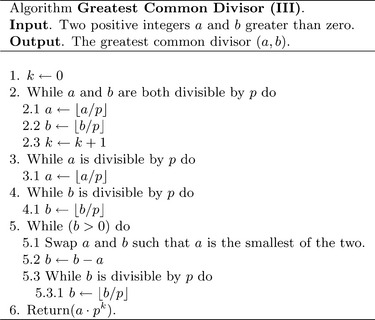
In particular, the value of p should be chosen such that the division in step 5.3.1 occurs often. It also helps that division by p be easy to compute. The ideal choice of p is two since division by two amounts to a right logical shift. Another important observation is that by step 5 both a and b are odd. Therefore, the difference b− a must be even, which means that each iteration removes one bit from the largest of the pair.
9.1.1 Complete Greatest Common Divisor
The algorithms presented so far cannot handle inputs that are zero or negative. The following algorithm can handle all input cases properly and will produce the greatest common divisor.
Algorithm mp_gcd. This algorithm will produce the greatest common divisor of two mp_ints a and b. It was originally based on Algorithm B, of Knuth [1, pp. 338] but has been modified to be simpler to explain. In theory, it achieves the same asymptotic working time as Algorithm B, and in practice, this appears to be true (Figure 9.4).
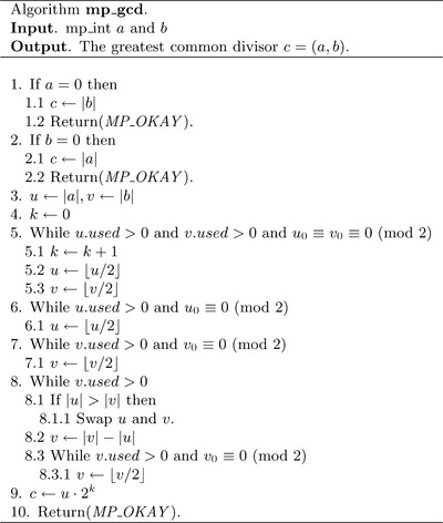
The first two steps handle the cases where either one or both inputs are zero. If either input is zero, the greatest common divisor is the largest input or zero if they are both zero. If the inputs are not trivial, u and v are assigned the absolutevalues of a and b, respectively, and the algorithm will proceed to reduce the pair.
step 5 will divide out any common factors of two and keep track of the count in the variable k. After this step, two is no longer a factor of the remaining greatest common divisor between u and v and can be safely evenly divided out of either whenever they are even. Steps 6 and 7 ensure that the u and v, respectively, have no more factors of two. At most, only one of the while loops will iterate since they cannot both be even.
By step 8 both u and v are odd, which is required for the inner logic. First, the pair are swapped such that v is equal to or greater than u. This ensures that the subtraction in step 8.2 will always produce a positive and even result. Step 8.3 removes any factors of two from the difference u to ensure that in the next iteration of the loop both are again odd.
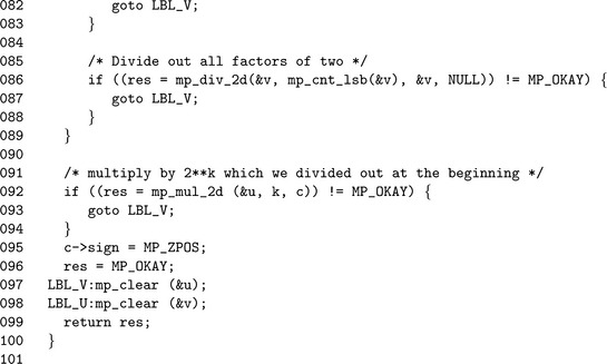
After v = 0 occurs the variable u has the greatest common divisor of the pair 〈 u, v〉 just after step 6. The result must be adjusted by multiplying by the common factors of two (2k) removed earlier.
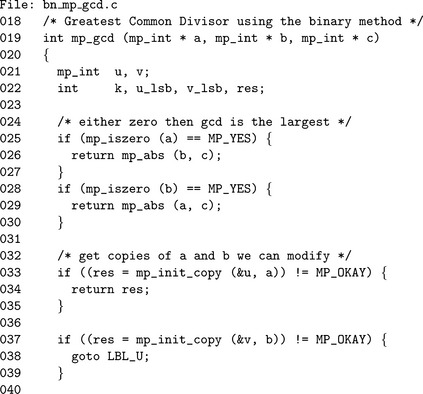
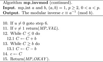
This function makes use of the macros mp_iszero and mp_iseven. The former evaluates to 1 if the input mp_int is equivalent to the integer zero; otherwise, it evaluates to 0. The latter evaluates to 1 if the input mp_int represents a non-zero even integer; otherwise, it evaluates to 0. Note that just because mp_iseven may evaluate to 0 does not mean the input is odd; it could also be zero. The three trivial cases of inputs are handled on lines 24 through 30. After those lines, the inputs are assumed non-zero.
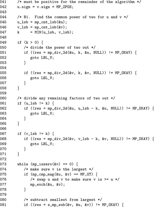
Lines 32 and 37 make local copies u and v of the inputs a and b respectively. At this point, the common factors of two must be divided out of the two inputs. The block starting at Line 44 removes common factors of two by first counting the number of trailing zero bits in both. The local integer k is used to keep track of how many factors of 2 are pulled out of both values. It is assumed that the number of factors will not exceed the maximum value of a C “int” data type1.
At this point, there are no more common factors of two in the two values. The divisions by a power of two on lines 62 and 68 remove any independent factors of two such that both u and v are guaranteed to be an odd integer before hitting themain body of the algorithm. The while loop on Line 73 performs the reduction of the pair until v is equal to zero. The unsigned comparison and subtraction algorithms are used in place of the full signed routines since both values are guaranteed to be positive and the result of the subtraction is guaranteed to be non-negative.
9.2 Least Common Multiple
The least common multiple of a pair of integers is their product divided by their greatest common divisor. For two integers a and b the least common multiple is normally denoted as [a, b] and numerically equivalent to (![]() For example, if a= 2 · 2 · 3 = 12 and b= 2 · 3 · 3 · 7 = 126, the least common multiple is
For example, if a= 2 · 2 · 3 = 12 and b= 2 · 3 · 3 · 7 = 126, the least common multiple is ![]()
The least common multiple arises often in coding theory and number theory. If two functions have periods of a and b, respectively, they will collide, that is be in synchronous states, after only [a, b] iterations. This is why, for example, random number generators based on Linear Feedback Shift Registers (LFSR) tend to use registers with periods that are co-prime (e.g., the greatest common divisor is 1.). Similarly, in number theory if a composite n has two prime factors p and q, then maximal order of any unit of ![]() will be [p−1, q−1].
will be [p−1, q−1].
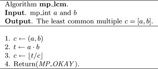
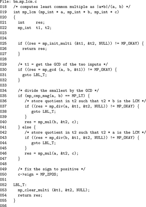
Algorithm mp_lcm. This algorithm computes the least common multiple of two mp_int inputs a and b. It computes the least common multiple directly by dividing the product of the two inputs by their greatest common divisor (Figure 9.5).
9.3 Jacobi Symbol Computation
To explain the Jacobi Symbol we will first discuss the Legendre function off which the Jacobi symbol is defined. The Legendre function computes whether an integer a is a quadratic residue modulo an odd prime p. Numerically it is equivalent to equation 9.1.
Theorem.Equation 9.1 correctly identifies the residue status of an integer a modulo a prime p.
Proof. Adapted from [21, pp. 68]. An integer a is a quadratic residue if the following equation has a solution.
Consider the following equation.
Whether equation 9.2 has a solution or not, equation 9.3 is always true. If a(p−1)/2−1 = 0 (mod p), then the quantity in the braces must be zero. By reduction,
As a result there must be a solution to the quadratic equation, and in turn, a must be a quadratic residue. If a does not divide p and a is not a quadratic residue, then the only other value a(p−1)/2 may be congruent to is−1 since
One of the terms on the right-hand side must be zero.
9.3.1 Jacobi Symbol
The Jacobi symbol is a generalization of the Legendre function for any odd non−prime moduli p greater than 2. If ![]() , then the Jacobi symbol
, then the Jacobi symbol ![]() is equal to the following equation.
is equal to the following equation.
By inspection if p is prime, the Jacobi symbol is equivalent to the Legendre function. The following facts2will be used to derive an efficient Jacobi symbol algorithm. Where p is an odd integer greater than two and ![]() , the following are true.
, the following are true.
Using these facts if a= 2k. a′ then
Subsequently, by fact three since p ≡ (p mod a) (mod a), then
By putting both observations into equation 9.7, the following simplified equation is formed.
The value of ![]() can be found using the same equation recursively.
can be found using the same equation recursively.
The value of ![]() equals 1 if k is even; otherwise, it equals
equals 1 if k is even; otherwise, it equals ![]() . Using this approach the factors of p do not have to be known. Furthermore, if (a, p) = 1, then the algorithm will terminate when the recursion requests the Jacobi symbol computation of
. Using this approach the factors of p do not have to be known. Furthermore, if (a, p) = 1, then the algorithm will terminate when the recursion requests the Jacobi symbol computation of ![]() , which is simply 1.
, which is simply 1.
Algorithm mp_jacobi. This algorithm computes the Jacobi symbol for an arbitrary positive integer a with respect to an odd integer p greater than three. The algorithm is based on algorithm 2.149 of HAC [2, pp. 73] (Figure 9.6).
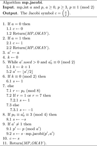
Steps 1 and 2 handle the trivial cases of a = 0 and a = 1, respectively. step 5 determines the number of two factors in the input a. If k is even, the term ![]() must always evaluate to one. If k is odd, the term evaluates to one if p0 iscongruent to one or seven modulo eight; otherwise, it evaluates to−1. After the
must always evaluate to one. If k is odd, the term evaluates to one if p0 iscongruent to one or seven modulo eight; otherwise, it evaluates to−1. After the ![]() term is handled, the (−1)(p−1)(a′−1)/4 is computed and multiplied against the current product s. The latter term evaluates to one if both p and a′ are congruent to one modulo four; otherwise, it evaluates to negative one.
term is handled, the (−1)(p−1)(a′−1)/4 is computed and multiplied against the current product s. The latter term evaluates to one if both p and a′ are congruent to one modulo four; otherwise, it evaluates to negative one.
By step 9 if a′ does not equal one a recursion is required. Step 9.1 computes p′≡ p(mod a′) and will recurse to compute ![]() , which is multiplied against the current Jacobi product.
, which is multiplied against the current Jacobi product.
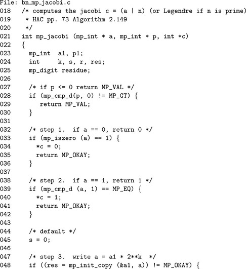
As a matter of practicality the variable a′ as per the pseudo-code is represented by the variable al since the ′ symbol is not valid for a C variable name character.
The two simple cases of a = 0 and a = 1 are handled at the very beginning to simplify the algorithm. If the input is non-trivial, the algorithm has to proceed and compute the Jacobi. The variable s is used to hold the current Jacobi product. Note that s is merely a C “int” data type since the values it may obtain are merely−1, 0 and 1.
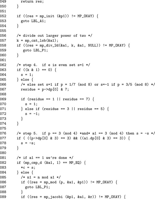
After a local copy of a is made, all the factors of two are divided out and the total stored in k. Technically, only the least significant bit of k is required; however, it makes the algorithm simpler to follow to perform an addition. In practice, an exclusive-or and addition have the same processor requirements, and neither is faster than the other.
Lines 62 through 73 determine the value of ![]() . If the least significant bit of k is zero, then k is even and the value is one. Otherwise, the value of s depends on which residue class p belongs to modulo eight. The value of (−1)(p−1)(a′−1)/4is computed and multiplied against s on lines 76 through 91.
. If the least significant bit of k is zero, then k is even and the value is one. Otherwise, the value of s depends on which residue class p belongs to modulo eight. The value of (−1)(p−1)(a′−1)/4is computed and multiplied against s on lines 76 through 91.
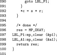
Finally, if a 1 does not equal one, the algorithm must recurse and compute ![]() .
.
9.4 Modular Inverse
The modular inverse of a number refers to the modular multiplicative inverse. For any integer a such that (a, p) = 1 there exists another integer b such that ab≡ 1 (mod p). The integer b is called the multiplicative inverse of a which is denoted as b = a−1. Modular inversion is a well-defined operation for any finitering or field, not just for rings and fields of integers. However, the former will be the matter of discussion.
The simplest approach is to compute the algebraic inverse of the input; that is, to compute b = aΦ(p)−1. If Φ(p) is the order of the multiplicative subgroup modulo p, then b must be the multiplicative inverse of a-the proof of which is trivial.
However, as simple as this approach may be it has two serious flaws. It requires that the value of F(p) be known, which if p is composite requires all of the prime factors. This approach also is very slow as the size of p grows.
A simpler approach is based on the observation that solving for the multiplicative inverse is equivalent to solving the linear Diophantine3equation.
Where a, b, p, and q are all integers. If such a pair of integers 〈 b, q〉 exists, b is the multiplicative inverse of a modulo p. The extended Euclidean algorithm (Knuth [1, pp. 342]) can be used to solve such equations provided (a, p) = 1. However, instead of using that algorithm directly, a variant known as the binary Extended Euclidean algorithm will be used in its place. The binary approach is very similar to the binary greatest common divisor algorithm, except it will produce a full solution to the Diophantine equation.
9.4.1 General Case
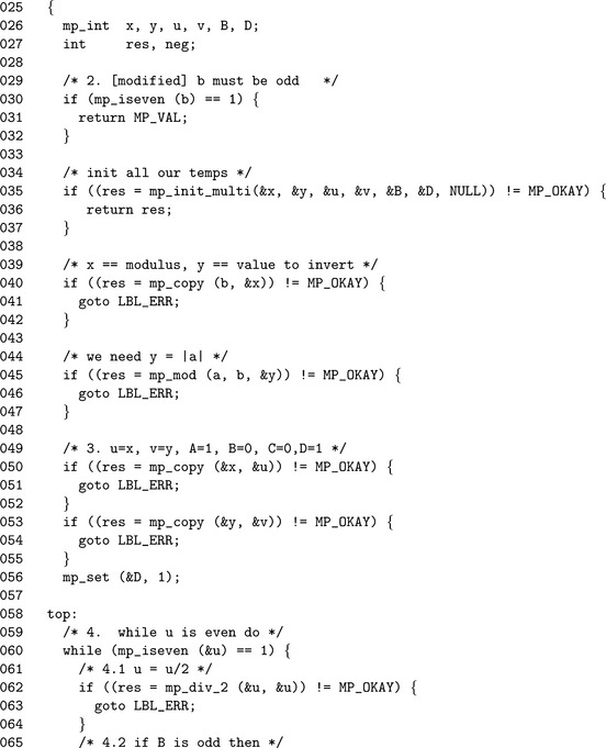
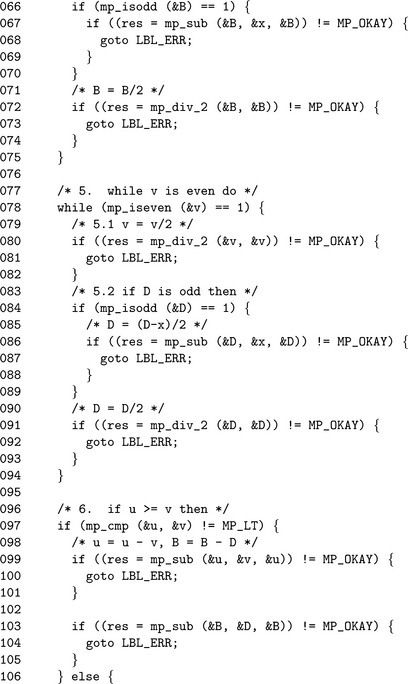
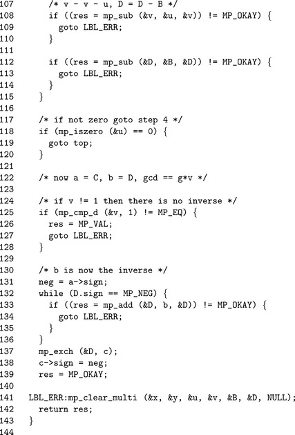
Algorithm mp_invmod. This algorithm computes the modular multiplicative inverse of an integer a modulo an integer b. It is a variation of the extended binary Euclidean algorithm from HAC [2, pp. 608], and it has been modified to only compute the modular inverse and not a complete Diophantine solution (Figure 9.7).
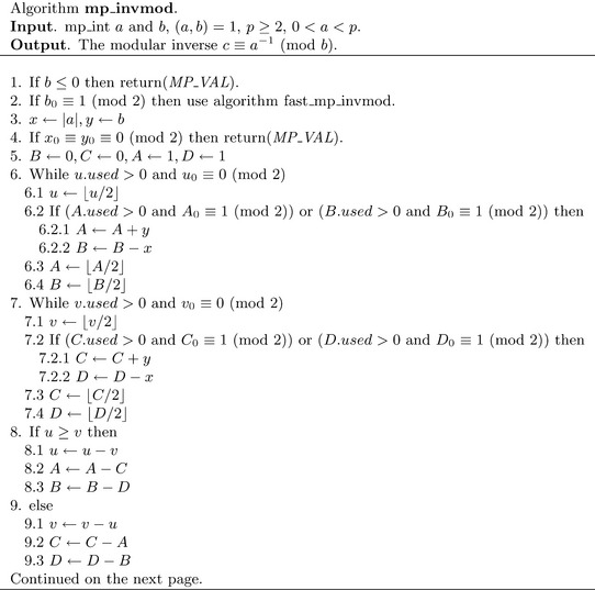
If b≤ 0, the modulus is invalid and MP_VAL is returned. Similarly if both a and b are even, there cannot be a multiplicative inverse for a and the error is reported.
The astute reader will observe that steps 7 through 9) are very similar to the binary greatest common divisor algorithm mp_gcd. In this case, the other variables to the Diophantine equation are solved. The algorithm terminates when u = 0, in which case the solution is
If v, the greatest common divisor of a and b, is not equal to one, then the algorithm will report an error as no inverse exists. Otherwise, C is the modular inverse of a. The actual value of C is congruent to, but not necessarily equal to, the ideal modular inverse, which should lie within 1 = a−1< b. Steps 12 and 13 adjust the inverse until it is in range. If the original input a is within 0< a< p, then only a couple of additions or subtractions will be required to adjust the inverse.
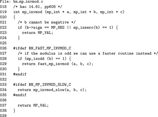
Odd Moduli
When the modulus b is odd the variables A and C are fixed and are not required to compute the inverse. In particular, by attempting to solve the Diophantine Cb + Da = 1, only B and D are required to find the inverse of a.
The algorithm fast_mp_invmod is a direct adaptation of algorithm mp_invmod with all steps involving either A or C removed. This optimization will halve the time required to compute the modular inverse.
9.5 Primality Tests
A non-zero integer a is said to be prime if it is not divisible by any other integer excluding one and itself. For example, a = 7 is prime since the integers 2 … 6 do not evenly divide a. By contrast, a = 6 is not prime since a = 6 = 2 · 3.
Prime numbers arise in cryptography considerably as they allow finite fields to be formed. The ability to determine whether an integer is prime quickly has been a viable subject in cryptography and number theory for considerable time. The algorithms that will be presented are all probabilistic algorithms in that when they report an integer is composite it must be composite. However, when the algorithms report an integer is prime the algorithm may be incorrect.
As will be discussed, it is possible to limit the probability of error so well that for practical purposes the probability of error might as well be zero. For the purposes of these discussions, let n represent the candidate integer of which the primality is in question.
9.5.1 Trial Division
Trial division means to attempt to evenly divide a candidate integer by small prime integers. If the candidate can be evenly divided, it obviously cannot be prime. By dividing by all primes 1< p ≤![]() , this test can actually prove whether an integer is prime. However, such a test would require a prohibitive amount of time as n grows.
, this test can actually prove whether an integer is prime. However, such a test would require a prohibitive amount of time as n grows.
Instead of dividing by every prime, a smaller, more manageable set of primes may be used instead. By performing trial division with only a subset of the primes less than ![]() +1, the algorithm cannot prove if a candidate is prime. However, often it can prove a candidate is not prime.
+1, the algorithm cannot prove if a candidate is prime. However, often it can prove a candidate is not prime.
The benefit of this test is that trial division by small values is fairly efficient, especially when compared to the other algorithms that will be discussed shortly. The probability that this approach correctly identifies a composite candidate when tested with all primes up to q is given by ![]() .
.
At approximately q = 30 the gain of performing further tests diminishes fairly quickly. At q = 90, further testing is generally not going to be of any practical use. In the case of LibTomMath the default limit q = 256 was chosen since it is not too high and will eliminate approximately 80% of all candidate integers. The constant PRIME_SIZE is equal to the number of primes in the test base. The array__prime_tab is an array of the first PRIME_SIZE prime numbers.
Algorithm mp_prime_is_divisible. This algorithm attempts to determine if a candidate integer n is composite by performing trial divisions (Figure 9.8).
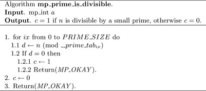
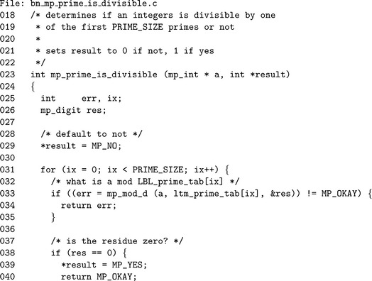
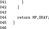
The algorithm defaults to a return of 0 in case an error occurs. The values in the prime table are all specified to be in the range of an mp_digit. The table__prime_tab is defined in the following file.
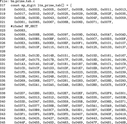
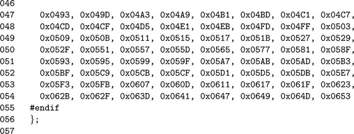
Note that there are two possible tables. When an mp_digit is 7-bits long, only the primes up to 127 may be included; otherwise, the primes up to 1619 are used. Note that the value of PRIME_SIZE is a constant dependent on the size of a mp_digit.
9.5.2 The Fermat Test
The Fermat test is probably one the oldest tests to have a non-trivial probability of success. It is based on the fact that if n is in fact prime, then an = a (mod n) for all 0< a< n. The reason being that if n is prime, the order of the multiplicative subgroup is n−1. Any base a must have an order that divides n−1, and as such, an is equivalent to a1 = a.
If n is composite then any given base a does not have to have a period that divides n−1, in which case it is possible that an an![]() a (mod n). However, this test is not absolute as it is possible that the order of a base will divide n−1, which would then be reported as prime. Such a base yields what is known as a Fermat pseudo-prime. Several integers known as Carmichael numbers will be a pseudo-prime to all valid bases. Fortunately, such numbers are extremely rare as n grows in size.
a (mod n). However, this test is not absolute as it is possible that the order of a base will divide n−1, which would then be reported as prime. Such a base yields what is known as a Fermat pseudo-prime. Several integers known as Carmichael numbers will be a pseudo-prime to all valid bases. Fortunately, such numbers are extremely rare as n grows in size.
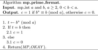
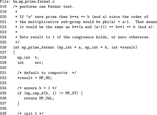
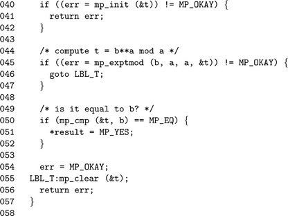
Algorithm mp_prime_fermat. This algorithm determines whether an mp_int a is a Fermat prime to the base b or not. It uses a single modular exponentiation to determine the result (Figure 9.9).
9.5.3 The Miller-Rabin Test
The Miller-Rabin test is another primality test that has tighter error bounds than the Fermat test specifically with sequentially chosen candidate integers. The algorithm is based on the observation that if n−1 = 2kr and if br ![]() ±1, then after up to k−1 squarings the value must be equal to−1. The squarings are stopped as soon as−1 is observed. If the value of 1 is observed first, it means that some value not congruent to ±l when squared equals one, which cannot occur if n is prime.
±1, then after up to k−1 squarings the value must be equal to−1. The squarings are stopped as soon as−1 is observed. If the value of 1 is observed first, it means that some value not congruent to ±l when squared equals one, which cannot occur if n is prime.
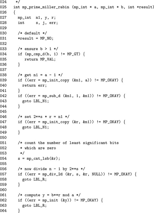
Algorithm mp_prime_miller_rabin. This algorithm performs one trial round of the Miller-Rabin algorithm to the base b. It will set c = 1 if the algorithm cannot determine if b is composite or c = 0 if b is provably composite. The values of s and r are computed such that a′ = a−1 = 2sr (Figure 9.10).
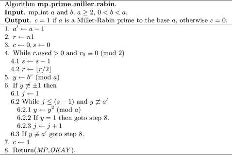
If the value y ≡bris congruent to ±1, then the algorithm cannot prove if a is composite or not. Otherwise, the algorithm will square y up to s−1 times stopping only when y ≡−1. If y2 ≡ 1 and y ≡ ±1, then the algorithm can report that a is provably composite. If the algorithm performs s−1 squarings and y ≡ −1, then a is provably composite. If a is not provably composite, then it is probably prime.

3. Devise and implement a method of computing the modular inverse of multiple numbers at once, by using a single inversion.
2. Look up and implement the “Almost Inverse” algorithm for integers. (Hint: Look in the IACR Crypto′95 proceedings.)
4. Devise and implement a method of generating random primes that avoids the need for trial division.
4. Devise and implement a method of generating large primes which are provably prime. Hint: Use a constructive approach to avoid the need for primality proof algorithms such as ECCP or AKS.
1Strictly speaking, no array in C may have more than entries than are accessible by an “int” so this is not a limitation.
2See HAC [2, pp. 72-74] for further details.
3See LeVeque [21, pp. 40-43] for more information.