
Exponentiation
Exponentiation is the operation of raising one variable to the power of another; for example,ab. A variant of exponentiation, computed in a finite field or ring, is called modular exponentiation. This latter style of operation is typically used in public key cryptosystems such as RSA and Diffie-Hellman. The ability to quickly compute modular exponentiations is of great benefit to any such cryptosystem, and many methods have been sought to speed it up.
7.1 Exponentiation Basics
A trivial algorithm would simply multiply a against itself b−1 times to compute the exponentiation desired. However, as b grows in size the number of multiplications becomes prohibitive. Imagine what would happen if b˜ 21024, as is the case when computing an RSA signature with a 1024-bit key. Such a calculation could never be completed, as it would take far too long.
Fortunately, there is a very simple algorithm based on the laws of exponents. Recall that lga(ab)=b and that lga(abac)=b+ c which are two trivial relationships between the base and the exponent. Let bi represent the i′th bit of b starting from the least significant bit. If b is a k–bit integer, equation 7.1 is true.
By taking the base a logarithm of both sides of the equation, equation 7.2 is the result.
The term a2i can be found from the i− 1′th term by squaring the term, since ![]() is equal to a2i+1. This observation forms the basis of essentially all fast exponentiation algorithms. It requires k squarings and on average k/2 multiplications to compute the result. This is indeed quite an improvement over simply multiplying by a a total of b−1 times.
is equal to a2i+1. This observation forms the basis of essentially all fast exponentiation algorithms. It requires k squarings and on average k/2 multiplications to compute the result. This is indeed quite an improvement over simply multiplying by a a total of b−1 times.
While this current method is considerably faster, there are further improvements to be made. For example, the a2i term does not need to be computed in an auxiliary variable. Consider the equivalent algorithm in Figure 7.1.
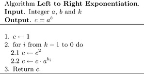
This algorithm starts from the most significant bit and works toward the least significant bit. When the i′th bit of b is set,a is multiplied against the current product. In each iteration the product is squared, which doubles the exponent of the individual terms of the product.
For example, let b= 1011002 = 4410. Figure 7.2 demonstrates the actions of the algorithm.
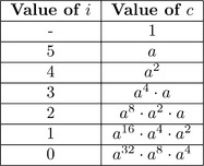
When the product a32.a8.a4 is simplified, it is equal to a44, which is the desired exponentiation. This particular algorithm is called “Left to Right” because it reads the exponent in that order. All the exponentiation algorithms that will be presented are of this nature.
7.1.1 Single Digit Exponentiation
The first algorithm in the series of exponentiation algorithms will be an unbounded algorithm where the exponent is a single digit. It is intended to be used when a small power of an input is required (e.g.,a5). It is faster than simply multiplying b−1 times for all values of b that are greater than three.
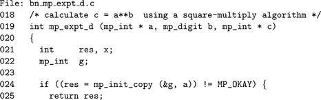
Algorithm mp_expt_d. This algorithm computes the value of a raised to the power of a single digit b. It uses the left to right exponentiation algorithm to quickly compute the exponentiation. It is loosely based on algorithm 14.79 of HAC [2, pp. 615], with the difference that the exponent is a fixed width (Figure 7.3).
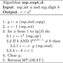
A copy of a is made first to allow destination variable c be the same as the source variable a. The result is set to the initial value of 1 in the subsequent step.
Inside the loop the exponent is read from the most significant bit first down to the least significant bit. First,c is invariably squared in step 3.1. In the following step, if the most significant bit of b is one, the copy of a is multiplied against c. The value of b is shifted left one bit to make the next bit down from the most significant bit the new most significant bit. In effect, each iteration of the loop moves the bits of the exponent b upwards to the most significant location.
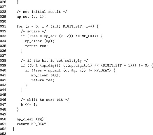
Line 29 sets the initial value of the result to 1. Next, the loop on Line 31 steps through each bit of the exponent starting from the most significant down toward the least significant. The invariant squaring operation placed on Line 33 is performed first. After the squaring the result c is multiplied by the base g if and only if the most significant bit of the exponent is set. The shift on Line 47 moves all of the bits of the exponent upwards toward the most significant location.
7.2 k–ary Exponentiation
When you are calculating an exponentiation, the most time-consuming bottleneck is the multiplications, which are in general a small factor slower than squaring.
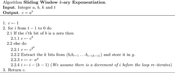
Recall from the previous algorithm that bi refers to the i′th bit of the exponent b. Suppose instead it referred to the i′th k–bit digit of the exponent of b. For k=1 the definitions are synonymous, and for k>1 algorithm 7.4 computes the same exponentiation. A group of k bits from the exponent is called a window, a small window on only a portion of the entire exponent. Consider the modification in Figure 7.4 to the basic left to right exponentiation algorithm.
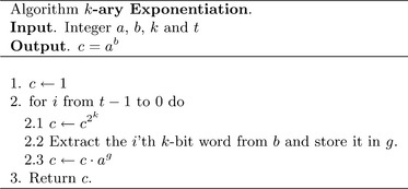
The squaring in step 2.1 can be calculated by squaring the value c successively k times. If the values of ag for 0< g<2khave been precomputed, this algorithm requires only t multiplications and tk squarings. The table can be generated with 2k−1−1 squarings and 2k−1 + 1 multiplications. This algorithm assumes that the number of bits in the exponent is evenly divisible by k. However, when it is not, the remaining 0< x = k− 1 bits can be handled with algorithm 7.1.
Suppose k=4 and t=100. This modified algorithm will require 109 multiplications and 408 squarings to compute the exponentiation. The original algorithm would on average have required 200 multiplications and 400 squarings to compute the same value. The total number of squarings has increased slightly but the number of multiplications has nearly halved.
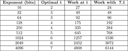
7.2.1 Optimal Values of k
An optimal value of k will minimize 2k +![]() n/k
n/k![]() + n − 1 for a fixed number of bits in the exponent n. The simplest approach is to brute force search among the values k=2, 3, …, 8 for the lowest result. Figure 7.5 lists optimal values of k for various exponent sizes and compares the number of multiplication and squaringsrequired against algorithm 7.1.
+ n − 1 for a fixed number of bits in the exponent n. The simplest approach is to brute force search among the values k=2, 3, …, 8 for the lowest result. Figure 7.5 lists optimal values of k for various exponent sizes and compares the number of multiplication and squaringsrequired against algorithm 7.1.
7.2.2 Sliding Window Exponentiation
A simple modification to the previous algorithm is only generate the upper half of the table in the range 2k−1![]() g<2k. Essentially, this is a table for all values of g where the most significant bit of g is a one. However, for this to be allowed in the algorithm, values of g in the range 0
g<2k. Essentially, this is a table for all values of g where the most significant bit of g is a one. However, for this to be allowed in the algorithm, values of g in the range 0![]() g<2k−1 must be avoided.
g<2k−1 must be avoided.
Figure 7.6 lists optimal values of k for various exponent sizes and compares the work required against algorithm 7.4.
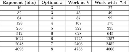
Similar to the previous algorithm, this algorithm must have a special handler when fewer than k bits are left in the exponent. While this algorithm requires the same number of squarings, it can potentially have fewer multiplications. The pre-computed table agis also half the size as the previous table.
Consider the exponent b= 1111010110010002 = 3143210, with k= 3 using both algorithms. The first algorithm will divide the exponent up as the following five 3-bit words b= (111, 101, 011, 001, 000)2. The second algorithm will break the exponent as b= (111, 101, 0, 110, 0, 100, 0)2. The single digit 0 in the second representation is where a single squaring took place instead of a squaring and multiplication. In total, the first method requires 10 multiplications and 18 squarings. The second method requires 8 multiplications and 18 squarings.
In general, the sliding window method is never slower than the generic k-ary method and often is slightly faster (Figure 7.7).
7.3 Modular Exponentiation
Modular exponentiation is essentially computing the power of a base within a finite field or ring. For example, computing d ≡![]() ab (mod c) is a modular exponentiation. Instead of first computing ab and then reducing it modulo c, the intermediate result is reduced modulo c after every squaring or multiplication operation.
ab (mod c) is a modular exponentiation. Instead of first computing ab and then reducing it modulo c, the intermediate result is reduced modulo c after every squaring or multiplication operation.
This guarantees that any intermediate result is bounded by 0![]() d
d![]() c2 − 2c+ 1 and can be reduced modulo c quickly using one of the algorithms presented in Chapter 7.
c2 − 2c+ 1 and can be reduced modulo c quickly using one of the algorithms presented in Chapter 7.
Before the actual modular exponentiation algorithm can be written a wrapper algorithm must be written. This algorithm will allow the exponent b to be negative, which is computed as c≡![]() (1/a)|b| (mod d). The value of (1/a) mod c is computed using the modular inverse (see Section 9.4). If no inverse exists, the algorithm terminates with an error.
(1/a)|b| (mod d). The value of (1/a) mod c is computed using the modular inverse (see Section 9.4). If no inverse exists, the algorithm terminates with an error.
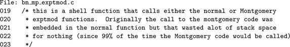
Algorithm mp_exptmod. The first algorithm that actually performs modular exponentiation is a sliding window k–ary algorithm that uses Barrett reduction to reduce the product modulo p. The second algorithm mp_exptmod_fast performs the same operation, except it uses either Montgomery or Diminished Radix reduction. The two latter reduction algorithms are clumped in the same exponentiation algorithm since their arguments are essentially the same (two mp_ints and one mp_digit)(Figure 7.8).
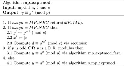
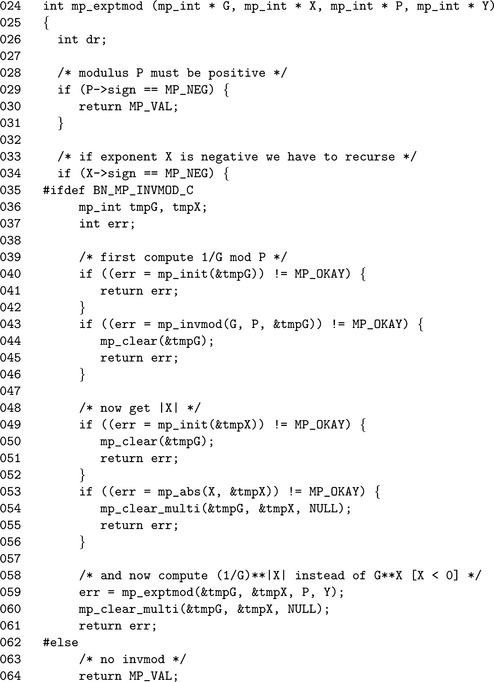

To keep the algorithms in a known state, the first step on Line 29 is to reject any negative modulus as input. If the exponent is negative, the algorithm tries to perform a modular exponentiation with the modular inverse of the base G. The temporary variable tmpG is assigned the modular inverse of G, and tmpX is assigned the absolute value of X. The algorithm will call itself with these new values with a positive exponent.
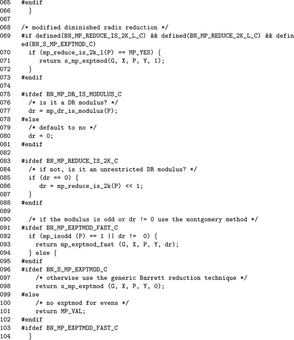
If the exponent is positive, the algorithm resumes the exponentiation. Line 77 determines if the modulus is of the restricted Diminished Radix form. If it is not, Line 86 attempts to determine if it is of an unrestricted Diminished Radix form. The integer dr will take on one of three values.
1. dr= 0 means that the modulus is not either restricted or unrestricted Diminished Radix form.
2. dr= 1 means that the modulus is of restricted Diminished Radix form.
3. dr= 2 means that the modulus is of unrestricted Diminished Radix form.
Line 49 determines if the fast modular exponentiation algorithm can be used. It is allowed if dr#0 or if the modulus is odd. Otherwise, the slower s_mp_exptmod algorithm is used, which uses Barrett reduction.
7.3.1 Barrett Modular Exponentiation
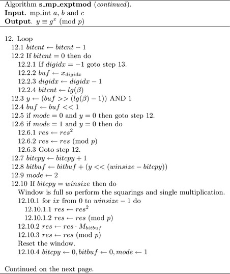
Algorithm s _mp_exptmod. This algorithm computes the x′th power of g modulo p and stores the result in y. It takes advantage of the Barrett reduction algorithm to keep the product small throughout the algorithm (Figure 7.9).
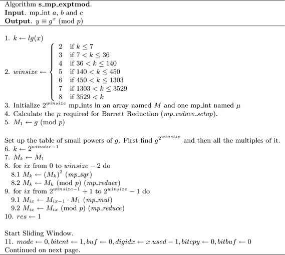
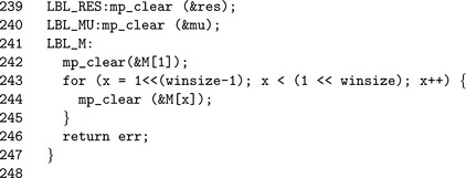
The first two steps determine the optimal window size based on the number of bits in the exponent. The larger the exponent, the larger the window size becomes. After a window size winsize has been chosen, an array of 2winsizemp_int variables is allocated. This table will hold the values of gx(mod p)for 2winsize− 1![]() x<2winsize.
x<2winsize.
After the table is allocated, the first power of g is found. Since g≥ p is allowed it must be first reduced modulo p to make the rest of the algorithm more efficient. The first element of the table at 2winsize−1 is found by squaring M1 successively winsize − 2 times. The rest of the table elements are found by multiplying the previous element by M1 modulo p.
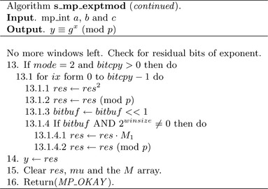
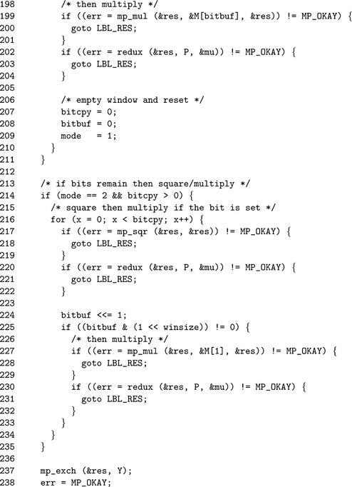
Now that the table is available, the sliding window may begin (Figure 7.10). The following list describes the functions of all the variables in the window.
1. The variable mode dictates how the bits of the exponent are interpreted.
(a) When mode= 0, the bits are ignored since no non-zero bit of the exponent has been seen yet. For example, if the exponent were simply1, then there would be lg(β) −1 zero bits before the first non–zero bit. In this case bits are ignored until a non–zero bit is found.
(b) When mode=1, a non–zero bit has been seen before and a new winsize–bit window has not been formed yet. In this mode, leading 0 bits are read and a single squaring is performed. If a non-zero bit is read, a new window is created.
(c) When mode=2, the algorithm is in the middle of forming a window and new bits are appended to the window from the most significant bit downwards.
2. The variable bitcnt indicates how many bits are left in the current digit of the exponent left to be read. When it reaches zero, a new digit is fetched from the exponent.
3. The variable buf holds the currently read digit of the exponent.
4. The variable digidx is an index into the exponent’s digits. It starts at the leading digit x.used−1 and moves toward the trailing digit.
5. The variable bitcpy indicates how many bits are in the currently formed window. When it reaches winsize the window is flushed and the appropriate operations performed.
6. The variable bitbuf holds the current bits of the window being formed.
step 12 is the window processing loop. It will iterate while there are digits available form the exponent to read. The first step inside this loop is to extract a new digit if no more bits are available in the current digit. If there are no bits left, a new digit is read, and if there are no digits left, the loop terminates.
After a digit is made available, step 12.3 will extract the most significant bit of the current digit and move all other bits in the digit upwards. In effect, the digit is read from most significant bit to least significant bit, and since the digits are read from leading to trailing edges, the entire exponent is read from most significant bit to least significant bit.
At step 12.5, if the mode and currently extracted bit y are both zero the bit is ignored and the next bit is read. This prevents the algorithm from having to perform trivial squaring and reduction operations before the first non–zero bit is read. Steps 12.6 and 12.7 through 12.10 handle the two cases of mode=1 and mode=2, respectively.
By step 13 there are no more digits left in the exponent. However, there may be partial bits in the window left. If mode=2 then a Left–to–Right algorithm is used to process the remaining few bits.
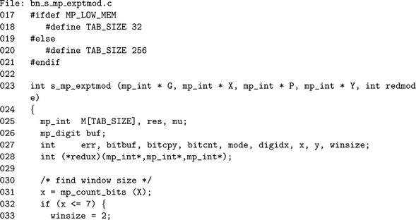
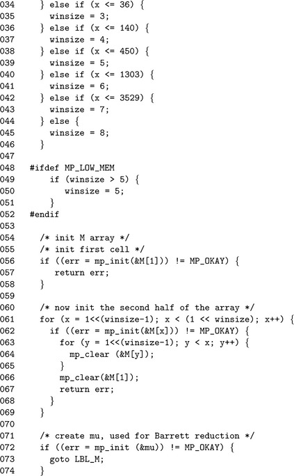
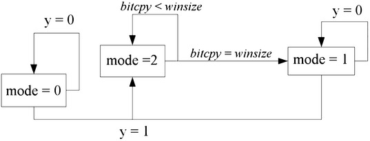
Lines 32 through 46 determine the optimal window size based on the length of the exponent in bits. The window divisions are sorted from smallest to greatest so that in each if statement, only one condition must be tested. For example, by the if statement on Line 38 the value of x is already known to be greater than 140.
The conditional piece of code beginning on Line 48 allows the window size to be restricted to five bits. This logic is used to ensure the table of precomputed powers of G remains relatively small.
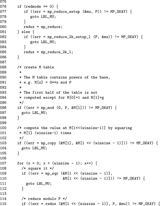
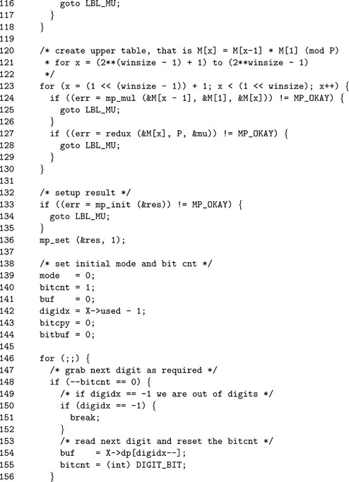
The for loop on Line 61 initializes the M array, while lines 72 and 77 through 86 initialize the reduction function that will be used for this modulus. Next, we populate (lines 88 through 129) the M table with the appropriate powers of g. At this point, we are ready to start the sliding window (lines 138 through 144), and begin processing bits of the exponent.
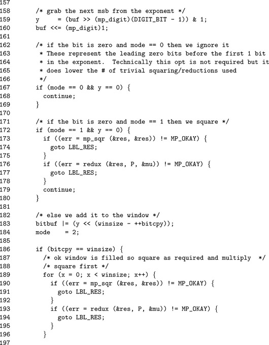
The first block of code inside the for loop extracts the next digit as required. We enter this loop initially in the state of requiring the next digit, which is why bitcnt is initially set to 1. Once we have a digit we can extract the most significant bit (Line 159). If the bit is zero, and we have not seen a non-zero bit yet we jump to the top of the loop. Otherwise, we either square and loop (lines 171 through 179) or add the bit to the window.
Note on Line 176 how we call the reduction function through our callback pointer redux. Provided the function has a consistent calling interface, it could be literally any sort of reduction function.
The block of code starting on Line 213 is used to handle cases where the window was not complete. In this case, we use a left–to–right exponentiation on single bits. Since the windows are small, this will involve doing at most 4 to 7 square-multiply steps which is acceptable given the runtime of the remainder of the algorithm.
7.4 Quick Power of Two
Calculating b=2a can be performed much quicker than with any of the previous algorithms. Recall that a logical shift left m![]() k is equivalent to m. 2k. By this logic, when m=1 a quick power of two can be achieved.
k is equivalent to m. 2k. By this logic, when m=1 a quick power of two can be achieved.
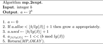
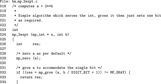
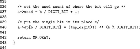
Algorithm mp_2expt. This algorithm computes a quick power of two by setting the desired bit of the result. It is used by various reduction functions such as Barrett and Montgomery (Figure 7.11).
2. Devise an algorithm to perform square and multiply exponentiation by reading the exponent from right to left.
5. Explore the use of exponent recoding (such as signed representations). Describe situations where it could be beneficial.
5. Devise an exponentiation algorithm which is does not leak timing information. Try to avoid using randomization.
5. Explore the use of vector addition chains. Develop a greedy encoding algorithm which can beat algorithm s_mp_exptmod for static (fixed), and then random exponents.